Performance Analysis of Three Intelligent Algorithms on Route Selection of Fishbone Layout

Abstract

The Internet of Things (IoT) has become an important strategy in the current round of global economic growth and technological development and provides a new path for the intelligent development of the logistics industry. With the development of the economy, the demand for logistics benefits is becoming more important. The appropriate use of technologies related to IoT to improve logistics efficiency, such as cloud computing, mobile computing and data mining, has become a topic of considerable research interest. Picking operations are currently an extremely important and cumbersome aspect of logistics center tasks. To shorten the picking distance and improve work efficiency, this paper uses the genetic algorithm, ant colony algorithm and cuckoo algorithm to optimize the picking path in a fishbone-layout warehouse and establishes an optimized model of the warehouse picking path under the fishbone layout. Data-mining technology is used to simulate the model and obtain the simulation data under the condition of multiple orders. The results provide a theoretical basis for the study of the fishbone-layout picking path model and has certain practical significance for the efficient operation of logistics enterprises. Through optimization, it is conducive to the sustainable development of enterprises and to achieving long-term profitability.

1. Introduction

Warehouse layout plays an important role in the logistics activities of the whole warehouse [1,2,3,4,5,6]. As a result, enterprises can obtain benefits by changing the layouts of their warehouses [7,8,9,10,11,12,13,14,15,16]. Reference [17] first questioned the traditional layout of shelves, where the fishbone layout was proposed and, under certain assumptions, it was verified that the fishbone layout reduced costs by an average of 23.5% compared with the traditional layout. Reference [18] pointed out that in terms of order selection, the fishbone layout is able to reduce the walking distance by 29.4% compared to the traditional layout. Therefore, it is of great significance to study the optimization of path picking for the fishbone layout. Government-funded studies of the picking path strategy for storage centers under the fishbone layout will improve the overall logistics development level of China to a certain extent, which is conducive to optimizing industrial structure and promoting the development of the national economy. For logistics enterprises, such research is capable of accelerating the response of customer demand, improving customer service satisfaction, enhancing overall operational efficiency, reducing logistics costs, enhancing the competitiveness of enterprises, and promoting the rapid and effective development of enterprises.

Compared with traditional algorithms, intelligent algorithms have certain advantages. In recent years, scholars at home and abroad have performed substantial research on intelligent algorithms. The genetic algorithm was first proposed by Professor J. Holland at the University of Michigan in 1975. Reference [19] used the genetic algorithm to optimize the storage of goods in warehouses. Reference [20] designed a greedy genetic algorithm to effectively solve the assignment and scheduling of vehicles. Reference [21] improved the basic genetic algorithm to solve or not layout optimization problems. Reference [22] can improve the optimization effect by improving the genetic operator. Reference [19] used the genetic algorithm to optimize the storage of goods in the warehouse, and used a warehouse that stores fast-moving consumer goods to carry out an example verification. Reference [23] designed a single-parent genetic algorithm based on improved genetic algorithm and applied it to solve the problem of picking optimization in automated warehouse. Reference [24] proposed the use of ABC method and adaptive hybrid genetic algorithm to solve the planning problem of warehousing in the storage area. Reference [25] applied the micro-genetic algorithm to the actual warehouse case. Reference [26] genetics algorithms have been used for analysis of logistics net in city logistics.

The ant colony algorithm was first proposed by the Italian scholar M. Dorigo et al. in 1991. Reference [27] used the ant colony algorithm to solve the rebalancing problem of the production line. In solving the scheduling problem of the production floor, reference [28] used genetic algorithms and ant colony algorithms to solve scheduling problems. Considering the problem of cargo recovery, reference [29] designed a hybrid ant colony algorithm to solve the problem of path optimization in such cases. The cuckoo search was proposed in 2009 by the British scholars [30,31,32]. Reference [33] proposed an ant colony algorithm with a three-level ladder structure, which effectively solved the problem of shop scheduling. Reference [34] made appropriate improvements to the parameters of the ant colony algorithm and improved the effectiveness of the algorithm.

Reference [35] improved the cuckoo algorithm to solve the problem of combinatorial optimization in warehouses and improved the convergence speed and accuracy of the algorithm. Reference [36] improved the cuckoo algorithm and applied the improved algorithm to solving the TSP problem. Finally, the correctness of the algorithm was verified. Reference [37] introduced the 2-opt optimization operator based on the traditional cuckoo algorithm, proposed an adaptive discrete cuckoo algorithm (ADCS) and effectively solved the picking path optimization problem of TSP problems. Reference [38] introduced the communication mechanism in the teacher-student communication algorithm into the cuckoo algorithm and applied it to solve the scheduling problem in the workshop. Reference [39] combined the penalty function method in the cuckoo algorithm and applied it to solve the optimization problem in practical engineering projects. Reference [40] applied the cuckoo algorithm to solve the multi-objective function optimization problem, and proposed a new multi-objective cuckoo search algorithm to improve the efficiency of algorithm calculation. Reference [41] added some features of collaborative search and adaptive search based on the cuckoo algorithm, and verified the effectiveness of the improved algorithm.

This paper uses the cuckoo algorithm because it appears recently, and no scholars have used it in the warehouse picking problem. Researchers have performed extensive research on intelligent algorithms and picking paths. Nevertheless, research on the fishbone layout is rare and has only appeared in recent years. For the layout of goods, in addition to the traditional layout, some scholars have proposed new layout strategies such as the flying-V, the inverted-V, and the fishbone layout [42,43,44,45,46,47]. In research on the order picking path, there are currently six main types, namely, the S-type strategy, the return-type strategy, the midpoint return transformation strategy, the maximum interval strategy, the combined strategy and the optimal strategy. Most of the research on the optimization of goods picking paths is based on the minimum total picking time. The intelligent optimization methods selected include the heuristic algorithm, the neural network method, the genetic algorithm, the tabu search method, the ant colony algorithm and the simulated annealing algorithm. We found that intelligent optimization algorithms are often used in path optimization problems. In automated warehouses, intelligent optimization algorithms are mostly used to solve stacker picking problems. Due to the lack of research on the fishbone layout, few scholars have used such algorithms in the selection and optimization of fishbone layout.

Compared with traditional algorithms, intelligent algorithms have certain advantages. Intelligent algorithms can give satisfactory solutions to complex, constrained, nonlinear, and multiextremity global optimization problems in a short time. In recent years, researchers have performed extensive research on intelligent algorithms, and new algorithms are constantly being proposed. Therefore, it is very meaningful to study the application of intelligent algorithms to the selection problem. Reference [48] proposed a method for optimizing the layout of different sizes of goods and used genetic algorithms to optimize the costs of picking operations and the like. Eleonora Bottani and others used genetic algorithms to optimize the storage of goods in a warehouse and used a warehouse that stores fast-moving consumer goods to carry out a case study, which not only reduced costs but also improved efficiency. The fishbone-layout picking path optimization problem is consistent with the traveling salesman problem, and the intelligent algorithm has obvious advantages in solving such problems. The genetic algorithm, ant colony algorithm, and cuckoo algorithm were applied to solve the optimization problem of the picking path in this paper. The first two algorithms have been applied to picking optimization problems, but there are no scholars that have applied the cuckoo algorithm to solve the problems of warehouse picking [49]. Therefore, it is also valuable to conduct research in this area.

In this paper, the intelligent optimization algorithms of the genetic algorithm, ant colony algorithm and cuckoo algorithm are applied to the optimization problem of the fishbone-layout picking path, which may benefit fishbone layout research. In particular, the application of the cuckoo algorithm provides a theoretical basis for the better application of the cuckoo algorithm in solving warehouse picking problems in the future. By using the intelligent optimization algorithm for the simulation calculations, the fishbone layout is approximated optimally on the picking path, which provides ideas for the subsequent optimization of the picking path with fishbone layout parameters. The establishment of the hybrid picking path model of the fishbone layout provides a decision-making basis for the efficient management and optimization control of the warehouse system and provides new ideas and methods for supply chain management theory and the basic operations technology of logistics distribution.

2. Construction of a Picking Path Model under a Fishbone Layout

2.1. Parameter Design of Fishbone Layout

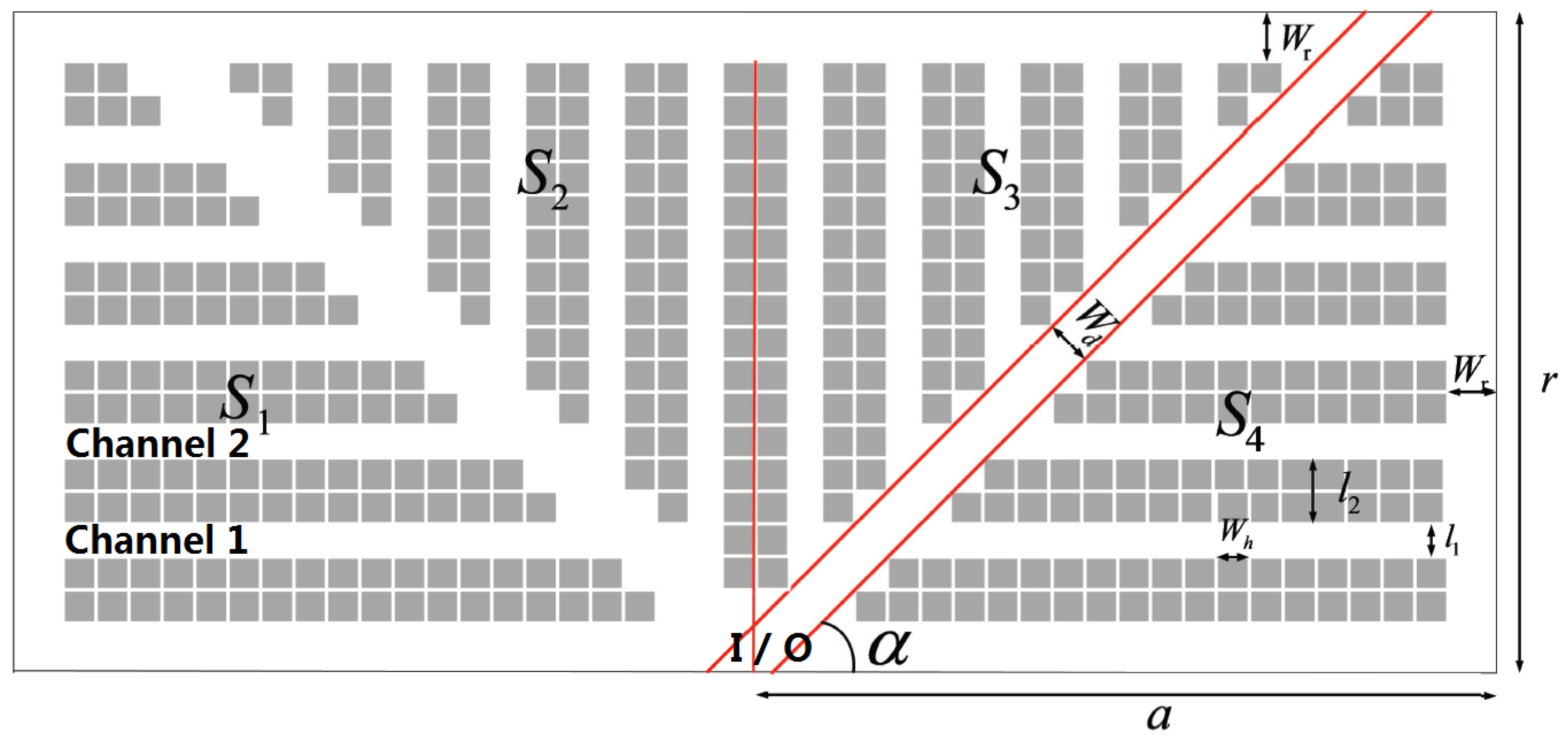
Setting the parameters of the fishbone layout is a prerequisite for the optimization of the picking path. A fishbone diagram is shown in Figure 1.

The parameters of this article are set as follows:

• $r:$ Width of the warehouse;
• $a:$ Half length of the warehouse;
• $W_r:$ Width of the cross aisle on both sides and the rear cross aisle;
• $W_d:$ Width of two diagonal aisles (main aisle);
• $l_1:$ Width of the picking aisle;
• $l_2:$ Width of double row shelves;
• $W_h:$ Length of the diagonal aisle (main aisle);
  $\alpha :$ Angle of the diagonal aisle (main aisle); and
  $S_1,S_2,S_3,S_4:$ Four pick zones divided by the two diagonal aisles and the warehouse centerline

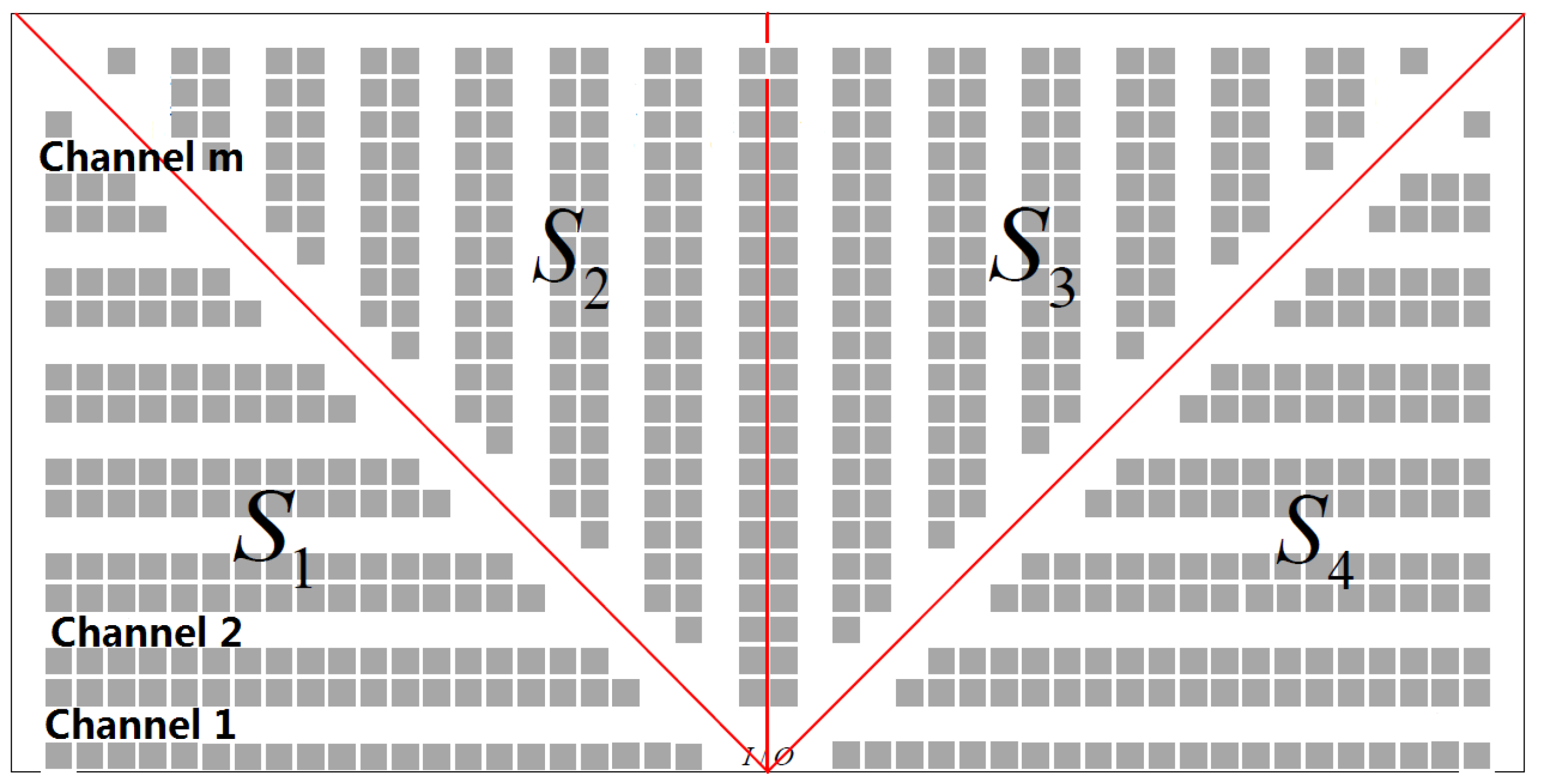
In order to construct the optimization model of the fishbone layout picking path problem, this paper designs the fishbone layout warehouse, as shown in Figure 2 below:

In addition, some assumptions about the picking environment of the warehouse need to be made before the model is established. The specific assumptions are as follows.

(1)

When the picking operator picks, he must start from the I/O point. After picking is completed, he must return to the I/O point. The two parts of the warehouse are symmetrical around the center.

(2)

The space between parallel shelves is called the picking aisle. The space between Zone 1 and Zone 2 is the main aisle, namely, the diagonal aisle. The space without shelves at the back of the warehouse and the space without shelves at the side of the warehouse are collectively called the aisles, namely, the rear aisles and the cross aisles on both sides of the warehouse.

(3)

The cargo is stored on the shelves, and the shelves are made up of a variety of openings. The length and width of each opening are the same, and the height of the shelves is not considered.

(4)

In regard to picking walking distances, we only consider the distance to walk to the location of the cargo, and the distance in the vertical direction is negligible. The picking aisle is a narrow aisle. The picker walks along the center of the passage. When the picker picks items on shelves on both sides of the aisle, the left and right movement distances are usually not considered, and both sides can be selected.

(5)

In the process of picking, when it is necessary to pass through the diagonal aisle and the cross aisle, the picking personnel and equipment must walk along the centerline until entering another sorting aisle.

(6)

When the picking operator picks according to an order, items are selected according to the position of the goods stored in the opening. The picking operator only needs to walk to the fixed opening to pick, and the picking operation can only take place in the picking aisle.

(7)

Before selection, all orders will be satisfied, and there will be no shortage in the selection process.

(8)

The capacity of the equipment and the number of pickers are sufficient to meet the demand, that is, the items in each order are chosen at a time when equipment and pickers are available.

(9)

The selection of each item at a single location can be fulfilled at one time.

(10)

In the fishbone layout warehouse, $S1$, $S2$, $S3$ and $S4$ are symmetrical about the diagonal aisle.

(11)

$S1$, $S2$, $S3$, and $S4$ have the same number of picking aisles, and the number is m.

(12)

The angle of the diagonal aisle is $\alpha =$ ${45}^{\circ }$. The length and width of each opening are equal and are equal to the width of the picking aisle, that is, $W_h={\displaystyle \frac{1}{2}}{l}_2=l_1$ and $W_r=l_1$.

2.2. Construction of the Picking Path Model

Based on the parameters set in the fishbone layout and the assumptions set in the fishbone layout selection, the optimization model of the picking path established in this paper is as follows:

Objective function:

$$\begin{array}{c}\hfill D=\min (d_{01}{x}_{01}+\sum _{i=1}^n\sum _{j=1}^n{d}_{ij}{x}_{ij}+d_{n0}{x}_{n0})\end{array}$$

(1)

Restrictions:

$$\begin{array}{c}\hfill \sum _{i=1}^n{x}_{ij}=1,j=1,2,3,\dots ,n\end{array}$$

(2)

$$\begin{array}{c}\hfill \sum _{j=1}^n{x}_{ij}=1,i=1,2,3,\dots ,n\end{array}$$

(3)

$$\begin{array}{c}\hfill \sum _{i,j\in K}{x}_{ij}\le \left|K\right|-1,K\subset V\end{array}$$

(4)

$$\begin{array}{c}\hfill x_{ij}=0or1\end{array}$$

(5)

where: D indicates the total travel distance of the picker to complete a selection activity, $d_{ij}(1\le i,j\le n,i\ne j)$ represents the shortest distance between i and j, $d_{01}$ represents the distance from the $I/O$ point, which is the distance from the starting point to position i, and $d_{n0}$ represents the distance from the final destination back to the starting point.

The function (6) is given by

$$x_{ij}=\left\{\begin{array}{c}1,\mathrm{The}\mathrm{picker}\mathrm{goes}\mathrm{through}\mathrm{the}\mathrm{path}\mathrm{from}\mathrm{the}\mathrm{position}i\mathrm{to}\mathrm{the}\mathrm{position}j,\hfill \\ 0,\mathrm{Otherwise}.\hfill \end{array}\right.$$

(6)

The objective function (1) indicates that the total walking distance is the shortest distance in a single selection process. Equations (3) and (4) indicate that the locations to be picked are picked once and only once. $x_{01}$ and $x_{n0}$ indicate that the picker starts from point $I/O$ and returns to point $I/O$. The picker will certainly go through two paths, from position 0 to position 1 and from position n to position 0, so $x_{01}=1$ and $x_{n0}=1$. Formula (5) indicates that there is no small loop, that is, solutions with an incomplete path are removed.

2.3. The Distance between Any Two Picking Points in the Fishbone Layout

The optimization problem of the picking path in the fishbone layout warehouse is an NP hard problem, and we set the objective function as the shortest distance of the picking path. First, we assume that the sequence number of any picking point is ($s,x,y,z$), where $s=1,2,3,4$, represents the number of the zone where the object is located. $x=1,2,\dots ,m$, indicates the number of the aisle to be selected, and $x\le 7$ represents the number of aisles in the fishbone-layout warehouse. $y=0or1$, which represents the two sides of the aisle in which the object is to be selected. If the item is on the lower or right side of the aisle, then $y=0$. $z=1,2,3,\dots ,n$ indicates that the goods to be chosen are in opening n. The numbering method is such that the numbers of the openings near the side and rear aisles are 1, and numbers are sequentially given as $1,2,3,\dots ,n$. $I/O$ is set to $(0,0,0,0)$, and the number is 0. Now let us assume that there are any two picking points $P,Q$, and the parameters are $(s_i,x_i,y_i,z_i)$ and $(s_j,x_j,y_j,z_j)$. $d_{ij}$ is the distance between two points.

First, we calculate the solution for $d_{01}$. The number 1 is the first position to be picked, which can be any point N in the picking scheme, where the serial number is $(s_1,x_1,y_1,z_1)$:

The Equation (7) is given by

$$\begin{array}{c}\hfill d_{01}={\displaystyle \frac{{\displaystyle \frac{1}{2}}{l}_1+(x_1-1)l_1+{\displaystyle \frac{1}{2}}{l}_2+(x_1-1)l_2}{sin\alpha }}+{\displaystyle \frac{1}{2}}{W}_{d}sin\alpha +(21-3(x_1-1)-z_1+{\displaystyle \frac{1}{2}})W_h\end{array}$$

(7)

According to the assumptions of this paper, the above equation can simplified, as follows:

$$\begin{array}{c}\hfill d_{01}=((3\sqrt{2}-3)x_1-z_1+25-{\displaystyle \frac{3}{2}}\sqrt{2})l_1\end{array}$$

(8)

Let $d_{n0}$ denote the distance from the last picking point back to $I/O$, assuming that the number of points M is $(S_n,X_n,Y_n,Z_n)$. In this case, $d_{n0}$ can be solved as follows:

The Equation (9) is given by

$$\begin{array}{c}\hfill d_{n0}={\displaystyle \frac{{\displaystyle \frac{1}{2}}{l}_1+(x_n-1)l_1+{\displaystyle \frac{1}{2}}{l}_2+(x_n-1)l_2}{sin\alpha }}+{\displaystyle \frac{1}{2}}{W}_{d}sin\alpha +(21-3(x_n-1)-z_n+{\displaystyle \frac{1}{2}})W_h\end{array}$$

(9)

According to the assumption of this paper, the above equation is simplified, as follows:

$$\begin{array}{c}\hfill d_{n0}=((3\sqrt{2}-3)x_n-z_n+25-{\displaystyle \frac{3}{2}}\sqrt{2})l_1\end{array}$$

(10)

$d_{ij}$ represents the distance between any two picking points $P,Q$, and the solution process is shown as follows:

• When $P,Q$ are two points in the same picking aisle, that is, $x_i=x_j$, the solution process is as follows:

  $$\begin{array}{c}\hfill d_{ij}=|Z_i-Z_j|W_h\end{array}$$

  (11)
  Equivalent to the following formula,

  $$\begin{array}{c}\hfill d_{ij}=|Z_i-Z_j|l_1\end{array}$$

  (12)
• When $P,Q$ are two points in different picking aisles, the solution is divided into the following two cases:

  (1)

  From picking point P to Q through the diagonal aisle, we have the following:

  The Equation (13) is given by

  $$\begin{array}{c}\hfill d_{ij}={\displaystyle \frac{|x_i-x_j|(l_1+l_2)}{sin\alpha }}+(49-3(x_i+x_j)-(z_i+z_j))W_h+W_{d}sin\alpha \end{array}$$

  (13)

  According to the assumptions of this paper, the above equation can be simplified, as follows:

  $$\begin{array}{c}\hfill d_{ij}=(3\sqrt{2}|x_i-x_j|-3(x_i+x_j)-(z_i+z_j)+50)l_1\end{array}$$

  (14)

  (2)

  From picking point P to Q through the aisle on both sides or the rear aisle, we have the following:

  $$\begin{array}{c}\hfill d_{ij}=|x_i-x_j|(l_1+l_2)+(Z_i+Z_j-1)W_h+W_r\end{array}$$

  (15)

  According to the assumptions of this paper, the above equation can be simplified, as follows:

  $$\begin{array}{c}\hfill d_{ij}=(3|x_i-x_j|+(z_i+z_j))l_1\end{array}$$

  (16)

  In summary:

  The Equation (17) is given by

  $$\begin{array}{c}\hfill d_{ij}=\min \left\{\begin{array}{c}(3\sqrt{2}|x_i-x_j|-3(x_i+x_j)-(z_i+z_j)+50)l_1.\\ (3|x_i-x_j|+(z_i+z_j))l_1\end{array}\right.x_i,x_j\in M;z_i,z_j\in N\end{array}$$

  (17)

• When $P,Q$ are two points that are located in different picking zones, the following situations are discussed: (1) When $P,Q$ are two points that are distributed in the two different zones of zone 1 and zone 4, there are two optional paths for picking. (2) When $P,Q$ are distributed in the two different zones of zone 1 and zone 2 or zone 3 and zone 4, there are three optional paths for picking. (3) When $P,Q$ are distributed in the two different zones of zone 1 and zone 3 or zone 2 and zone 4, there are three optional paths for picking (assuming that P is in zone 1 and Q is in zone 3). (4) When $P,Q$ are two points that are distributed in the two different zones of zone 2 and zone 3, there are two optional paths for picking.

For example, when $P,Q$ are two points that are distributed in the two different zones of zone 1 and zone 4, there are two optional paths for picking:

(1)

Without the passage of the rear aisle, that is, after passing through aisle $x_i$ where Q is selected, we enter the diagonal aisle and then enter aisle $x_i$ where Q is selected. Then:

The Equation (18) is given by

$$\begin{array}{c}\hfill d_{ij}=(49-3x_i-3x_j-z_i-z_j)W_h+2W_{d}sin\alpha +l_2+{\displaystyle \frac{(x_i+x_j-2)(l_1+l_2)}{sin\alpha }}\end{array}$$

(18)

According to the assumption of this paper, the above equation can be simplified, as follows:

$$\begin{array}{c}\hfill d_{ij}=(53-6\sqrt{2}+(3\sqrt{2}-3)(x_i+x_j)-z_i-z_j)l_1\end{array}$$

(19)

(2)

With the passage of the rear aisle, that is, after passing through aisle where Q is selected, and after passing through zones 2 and 3, we enter the diagonal aisle and then enter aisle $x_j$ where Q is selected to be picked.

The Equation (20) is given by

$$\begin{array}{c}\hfill d_{ij}=(97-6x_i-6x_j-z_i-z_j)W_h+(sin\alpha +cos\alpha )W_d+W_r+(x_i+x_j-1)(l_1+l_2)\end{array}$$

(20)

According to the assumptions of this paper, the above equation can be simplified, as follows:

$$\begin{array}{c}\hfill d_{ij}=(97-3x_i-3x_j-z_i-z_j)l_1\end{array}$$

(21)

In summary:

The Equation (22) is given by

$$\begin{array}{c}\hfill d_{ij}=\min \left\{\begin{array}{c}{d}_{ij}=(53-6\sqrt{2}+(3\sqrt{2}-3)(x_i+x_j)-z_i-z_j)l_1\\ d_{ij}=(97-3x_i-3x_j-z_i-z_j)l_1\end{array}\right.x_i,x_j\in M;z_i,z_j\in N\end{array}$$

(22)

The above Equations (7)–(22) represent some solution of the distance between any two picking points in the fishbone layout warehouse. Due to the randomness of the goods in the picking order, different picking orders may have different picking paths depending on the picking strategy.

3. Calculation Steps of Three Intelligent Algorithms

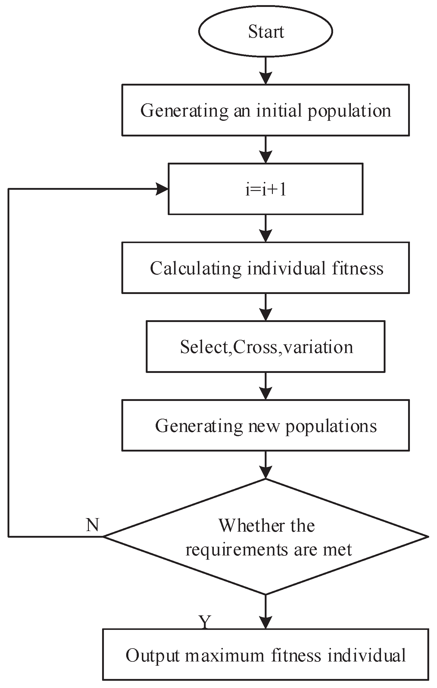
3.1. Genetic Algorithm Operation Steps

In the warehouse picking process, the specific implementation steps of the basic genetic algorithm are as follows:

(1)

First, generate the distance matrix of the coordinates of the goods to be picked and the distance traveled by any goods to be picked;

(2)

Randomly generate the initial population P(0);

(3)

According to the fitness function, find the fitness value in the initial population, determine the current optimal picking path, and calculate the total path length;

(4)

Select the crossover operation to generate new individuals and new populations; and

(5)

Determine whether the solution with the highest fitness in the new population satisfies the output condition. If yes, output the optimal solution; otherwise, return to step 3 to continue the iteration until the terminating condition is satisfied.

In the process of picking goods in the warehouse, the structural flow chart of the basic genetic algorithm is shown in Figure 3.

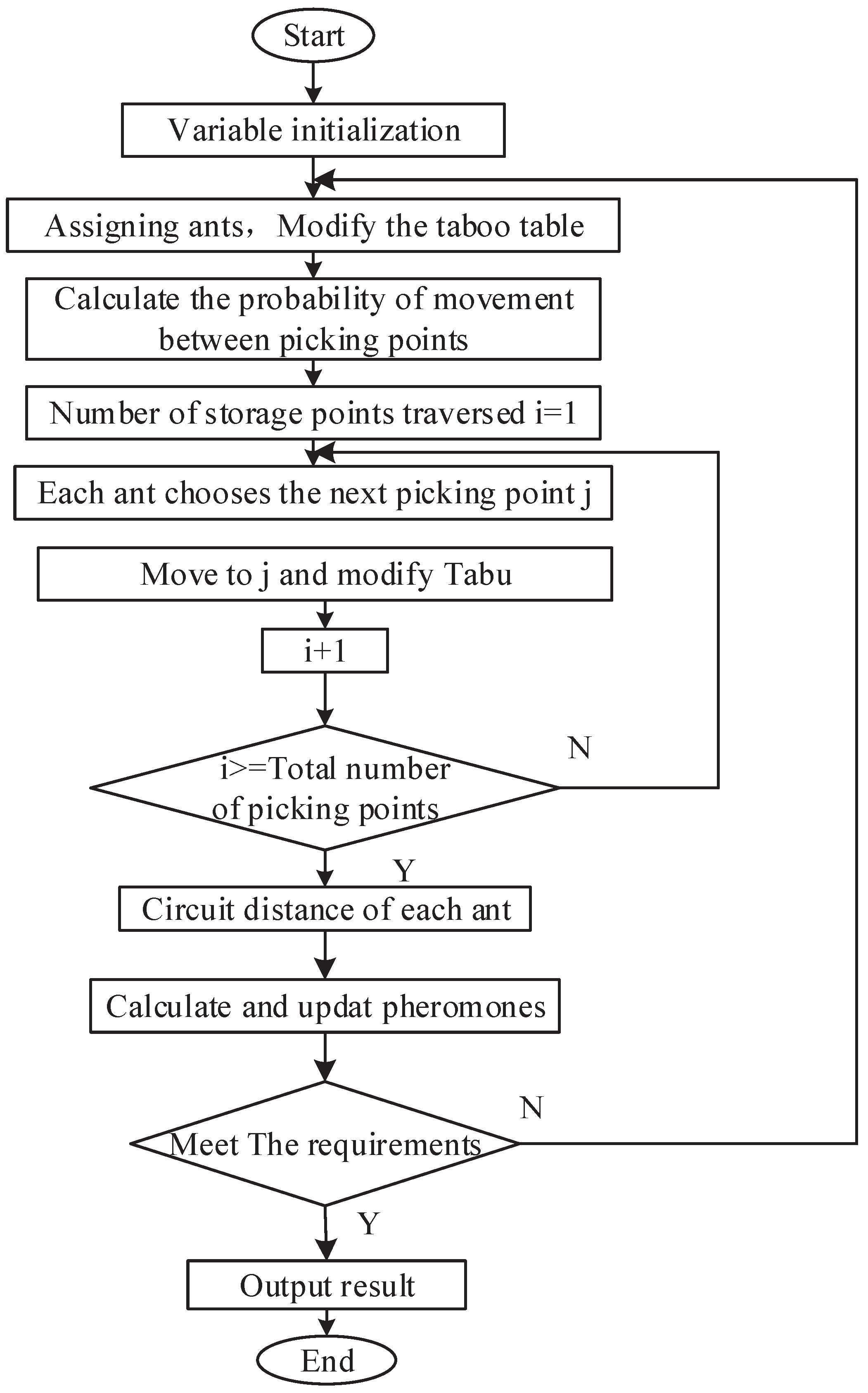
3.2. Ant Colony Algorithm Operation Steps

According to the previous research in the literature, we take the number of ants as the number of goods to be picked, and m ants are located in n storage places. After accessing store i, the ant moves to the next store based on the pheromone concentration function probability $p_{ij}^k$ on path j:

$$\begin{array}{c}\hfill p_{ij}^k=\left\{\begin{array}{c}{\displaystyle \frac{{\left[{\tau }_{ij}(t)\right]}^{\alpha }{\left[{\eta }_{ij}(t)\right]}^{\beta }}{{\sum }_{i\in allowe{d}_k}{\left[{\tau }_{ij}(t)\right]}^{\alpha }{\left[{\eta }_{ij}(t)\right]}^{\eta }}}j\in allowe{d}_k\\ 0others\end{array}\right.\end{array}$$

(23)

Among these parameters, $allowe{d}_k$ represents the set of all paths that ants can choose when walking to the next store, which changes with the progress of ant k. The amount of information ${\tau }_{ij}$ will gradually weaken with time, and ${\eta }_{ij}$ is the expectation of being transferred from store i to j.

To intuitively illustrate the realization of the ant colony algorithm, this article assumes the following symbolic descriptions:

• $m:$ The number of ants in the colony;
• $NC\_6\max :$ The maximum number of iterations;
• $C:$ The coordinates of n storage locations;
• $n:$ The number of the opening in which the goods to be picked are located;
• $Alpha:$ Parameters that indicate the importance of pheromones;
• $Beta:$ Parameters that indicate the significance of the heuristic factor;
• $Rho:$ Pheromone evaporation coefficient;
• $Q:$ Pheromone increase intensity coefficient;
• $Eta:$ Said heuristic;
• $Tau:$ Pheromone matrix;
• $R\_best:$ The best path from generation to generation;
• $L\_best:$ The length of the best path from generation to generation.

In the warehouse picking process, the specific implementation steps of the basic ant colony algorithm are as follows:

(1)

Initialize the parameters and set the amount of initial information for storage (goods);

(2)

Assign ants to the various selected goods and modify the ant taboo list $Tabu$;

(3)

According to the selection probability formula, calculate the moving probability of each picking point;

(4)

Each ant $k(k=1,2,3,\dots ,m)$ chooses the opening j according to the probability moving formula and modifies the ants’ tabu table $Tabu$;

(5)

If the ants have traversed all the selected openings, then proceed to step 6; otherwise, return to step 4.

(6)

Calculate the loop distance traveled by each ant, and calculate and update the intercity pheromone $Tau$;

(7)

If the stop condition is satisfied, then the loop is ended, and the result is output. Otherwise, the taboo list of each ant is deleted and the procedure returns to the second step.

In the warehouse picking process, the structural flow chart of the basic ant colony algorithm is shown in Figure 4.

3.3. Cuckoo Algorithm Operation Steps

A cuckoo bird randomly looks for the bird’s nest. In the Cuckoo Search algorithm, each egg represents a solution, and during initialization, a solution is created randomly. The cuckoo random walking equation is as follows:

$$\begin{array}{c}\hfill x_i^{(t+l)}=x_i^t+\alpha \oplus Levy(\lambda )\end{array}$$

(24)

where $x_i^t$ is the ith solution of the tth generation, $\alpha$ is the step information, ⊕ is the dot multiplication, and $Levy(\lambda )$ is the random search path, that is generated by the distribution. The $levy$ formula is as follows:

$$\begin{array}{c}\hfill levy-u=t^{-\lambda }(1<3)\end{array}$$

(25)

The specific formula for generating a new individual is as follows:

$$\begin{array}{c}\hfill v=v+Stepsiz{e}_j\times randn\left[D\right]\end{array}$$

(26)

where $randn\left[D\right]$ is the Gaussian distribution generated on $[1,D]$, where $Stepsiz{e}_j$ is calculated as follows:

$$\begin{array}{c}\hfill Stepsiz{e}_j=0.01{({\displaystyle \frac{u_j}{v_j}})}^{{\displaystyle \frac{1}{\lambda }}}(v-X_{best})\end{array}$$

(27)

Among the above parameters, $u=t^{-\lambda }\times randn\left[D\right]$, $v=randn\left[D\right]$, and v is initialized as $v=x_i^t$.

After the new program is generated, it needs to be compared with the original program, and the program with the lower fitness value will be reserved for the next generation.

In the event that a cuckoo’s egg is detected, the host bird’s selection and establishment of a new nest takes preference over random walk behavior, as follows:

$$\begin{array}{c}\hfill v_i=\left\{\begin{array}{c}{X}_i=rand(X_{r1}-X_{r2})rand<P_a\\ X_{i}otherwise\end{array}\right.\end{array}$$

(28)

In the CS algorithm, the solution is limited by the search space, Within this space, the lower bound of the population search is $X_{\min }=(x_{1,\min },x_{2,\min },\dots ,x_{D,\min })$, and the upper bound of the population search is $X_{\max }=(x_{1,\max },x_{2,\max },\dots ,x_{D,\max })$

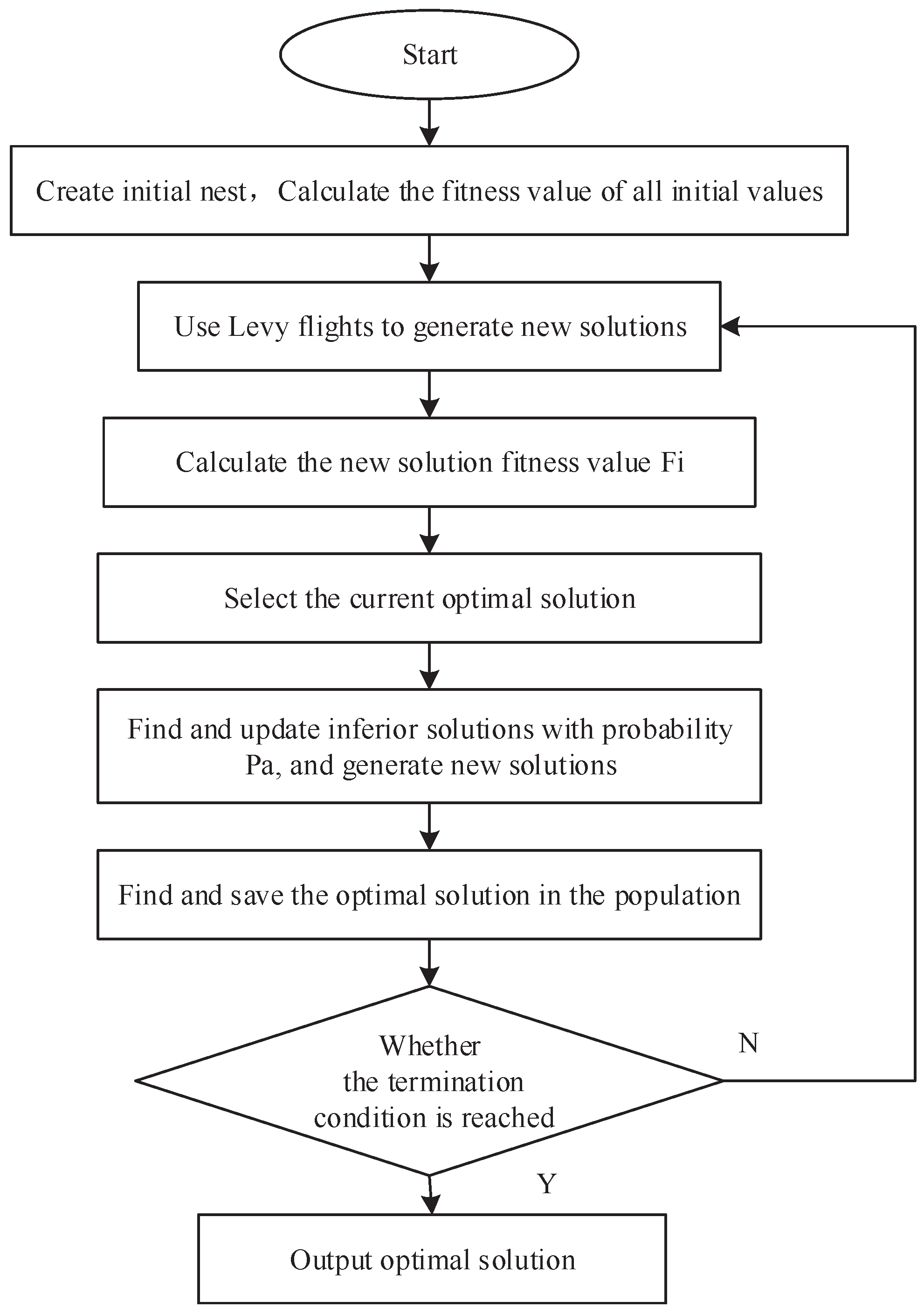
In the warehouse picking process, the structural flow chart of the basic cuckoo algorithm is shown in Figure 5.

A detailed description of the algorithm steps is as follows:

Step 1. Population initialization; randomly initialize the nest position $p_0=[x_1^{(0)},x_2^{(0)},\dots ,x_n^{(0)}]$, find the best bird location $x_{\mathrm{best}}^0$, and record the fitness value $f_{\min }$ of the optimal solution $x_{\mathrm{best}}^0$ simultaneously.

Step 2. Loop body

(1)

Keep the best birdhouse position $x_{\mathrm{best}}^{t-l}$ of the previous generation. Then use Formula (24) to update all nest locations and get a new set of nest locations, which is indicated as $p_t=[x_1^{(t)},x_2^{(t)},\dots ,x_n^{(t)}]$. After that, the selection operation is performed, and by comparing this result with the previous generation of bird’s nest positions $p_t-1=[x_1^{(t-1)},x_2^{(t-1)},\dots ,x_n^{(t-1)}]$, the bird’s nest position $g_t=[x_1^{(t)},x_2^{(t)},\dots ,x_n^{(t)}]$ with the best fitness value is selected.

(2)

The probability of a cuckoo’s egg being found is $p_a$, compare $p_a$ with $r\in [0,1]$. Save the nest location in $g_t$ that meets $p_a\le r$ and update the preserved nest location with Formula (28), Then the new nest location with the corresponding nest location in the middle of $g_t$. Choose the best bird nest location and keep it. This will yield a new set of better bird’s nest locations: $p_t=[x_1^{(t)},x_2^{(t)},\dots ,x_n^{(t)}]$.

Step 3. Update the population, Then, the fitness value of the optimal bird’s nest position $x_{\mathrm{best}}^t$ obtained from $p_t$ in (2) is compared with the optimal value $f_{\min }$. If the value is less than $f_{\min }$, update $f_{\min }$ and $g_{\mathrm{best}}$ simultaneously, if the value is not less than $f_{\min }$, then do not update $f_{\min }$ and $g_{\mathrm{best}}$. After that, if the stop condition is satisfied, the global optimal value $f_{\min }$ and the corresponding global optimal position $g_{\mathrm{best}}$ are output, and if the stop condition is not reached, the iteration is continued.

To visualize the cuckoo algorithm implementation process, this article uses the following symbols:

• $n:$ Indicates the number of host nests;
• $p_a:$ Indicates the probability that the nest is discovered by the host;
• $nd:$ Indicates the number of points to be picked in the fishbone layout;
• $N\_iter:$ Indicates the maximum number of iteration.

In the warehouse picking process, the concrete realization of the basic cuckoo algorithm is as follows:

(1)

Parameter initialization;

(2)

Generate initial nest, initialize all solutions of the population and calculate the fitness of all initial solutions;

(3)

Use the Levy flights method to generate new solutions;

(4)

Calculate the fitness of the new solution;

(5)

A candidate solution is randomly selected from the initial solution, and the solution with smaller fitness value is retained by comparing the fitness values of the candidate solution and the new solution;

(6)

Discover and update the inferior solutions with probability $p_a$, which result in new solutions;

(7)

All the optimal solutions remain in the next generation; find and save the optimal solution;

(8)

If the stop condition is satisfied, the loop is ended and the result is output; otherwise, return to step 3 to continue the iteration.

4. Comparison of the Performance of the Three Intelligent Algorithms

4.1. Solution Example

To facilitate the calculation, this chapter sets the width of the picking channel $l_1$ to 1. The genetic algorithm parameters are as follows: M = 100, $Cnum$ = 500, $Pc$ = 0.8, $Pmutation$ = 0.08. The ant colony algorithm parameters are as follows: $Alpha$ = 1, $Beta$ = 5, $Rho$ = 0.1, $NC\_\max$ = 500, Q = 100. The cuckoo algorithm parameters are as follows: n = 100, $Pa$ = 0.25, and $N\_iter$ = 500. In reality, due to the random arrival of customer orders, the optimization effect of picking different items is also different. For this reason, we randomly generated 100 storage positions for the points to be selected and randomly selected 10 orders, each containing 10, 20, 30 and 40 points to be selected for the calculations.

4.2. Comparison of the Performance of the Three Algorithms

The above 10, 20, 30, and 40 points for the selected orders were run through the three intelligent algorithms, and the results are summarized. The results of the comparisons are summarized in the following

Table 1. Summary of Results of The Initial Run.

Number of Picking Points	Method	CPU Running Time	Optimization Results	Equivalent to the S-Type to Improve the Distance	Quivalent to S-Type Improvement Ratio
10	S type	0	187.7	0	0
	GA	25.191099	160.97	26.73	14.24%
	ACO	2.984924	146.46	41.24	21.97%
	CS	33.538280	146.46	41.24	21.97%
20	S type	0	345.43	0	0
	GA	27.219359	330.94	14.49	4.19%
	ACO	10.568599	268.21	77.22	22.35%
	CS	3.196464	272.70	72.73	21.05%
30	S type	0	415.67	0	0
	GA	29.630254	491.15	−75.48	−18.16%
	ACO	28.910247	302.21	113.46	27.30%
	CS	3.524749	304.70	110.97	26.70%
40	S type	0	407.91	0	0
	GA	31.732872	607.37	−199.46	−48.90%
	ACO	62.150011	302.94	104.97	25.73%
	CS	3.585820	293.43	114.48	28.07%

,

Table 2. Summary of Operating Results with 10 Orders.

Order Path Distance		1	2	3	4	5	6	7	8	9	10
10	S type	188	203	196	175	184	207	192	183	177	231
	GA	161	165	170	148	152	171	159	167	142	206
	ACO	146	147	152	133	140	153	144	137	142	173
	CS	146	147	152	133	140	153	144	137	142	173
20	S type	345	373	321	349	330	345	362	297	308	319
	GA	331	347	301	317	305	309	338	257	274	301
	ACO	268	289	276	265	274	263	287	226	246	248
	CS	273	280	282	247	274	273	269	233	237	257
30	S type	416	471	445	408	433	396	421	439	418	427
	GA	491	503	429	561	482	430	491	464	583	529
	ACO	302	367	328	310	354	301	307	318	301	316
	CS	305	359	307	321	341	301	313	329	297	318
40	S type	408	499	439	419	476	461	430	463	408	437
	GA	607	709	633	672	584	496	549	683	491	539
	ACO	303	374	319	296	373	351	319	320	296	317
	CS	293	368	323	304	364	347	313	312	293	309

and

Table 3. Optimization Ratio Summary Table.

Grouping	GA				ACO				CS
	10	20	30	40	10	20	30	40	10	20	30	40
<0	0	0	9	10	0	0	0	0	0	0	0	0
0–10%	1	7	1	0	0	0	0	0	1	0	0	0
10–20%	9	3	0	0	10	2	1	9	9	3	0	9
20–30%	0	0	0	0	0	8	9	1	0	7	9	1
30–40%	0	0	0	0	0	0	0	0	0	0	1	0
Total	10	10	10	10	10	10	10	10	10	10	10	10

:

In the optimization of fishbone-layout warehouse picking, when the number of points to be picked is 10, the basic genetic algorithm can effectively optimize the path. When the number of points to be selected increases to 30 and 40, the basic genetic algorithm already does not output the optimum results, which is negative compared with the S-picking strategy. It can be concluded that the basic genetic algorithm easily falls into the local optimal solution in the process of computing, and it is difficult to escape the local optimal solution. When the number of points to be picked increases, the optimization efficiency of the ant colony algorithm for the picking path is stable at 20–30% compared with that of the S-picking strategy. However, the cuckoo algorithm has the same effect on the optimization of the picking path of a fishbone-layout warehouse as does the ant colony optimization algorithm. When the number of picking points increases gradually, the cuckoo algorithm is more stable, and as the number of points to be picked increases, the optimization effect is more obvious.

Second, with respect to the CPU running time, the average computing time of the genetic algorithm is very long, and as the number of points to be picked increases, the computing time tends to increase gradually. When the number of picking points increases from 10 to 40, the CPU running time of the algorithm is almost exponentially extended. In contrast, the CPU running time of the cuckoo algorithm is maintained at a very low level of only 3.5 s, and it can be seen that the cuckoo algorithm’s run time is not affected by the number of points to be selected.

Finally, it can be seen from the algorithm iteration and the result optimization graph that the genetic algorithm converges slowly and is unstable with an increase in the number of iterations. The ant colony algorithm converges fast in the early iterations, but the latter effect is not obvious, and as the number of points to be picked increases, the number of iterations needed to obtain the optimal solution steadily increases. While the cuckoo algorithm shows a steady convergence in the early and late iterations of the algorithm, as the number of points to be picked increases, the number of iterations needed to reach the optimal solution also steadily increases.

Based on the above analysis, when the number of points to be picked is less than 20, all three kinds of intelligent algorithms can be used to optimize the picking path. When the number of points to be picked is more than 20, the picking path optimization effect of the ant colony algorithm and cuckoo algorithm are obvious. Thus, it can be concluded that the cuckoo algorithm is the best, followed by the ant colony algorithm, and finally the genetic algorithm when optimizing the picking path of a fishbone-layout warehouse.

5. Conclusions

This paper carried out the following research work. In view of the characteristics of the fishbone-layout picking channel, a picking path optimization model was designed. The fishbone layout changes the traditional arrangement of shelves. In this paper, for convenience, the fishbone shelf layout is divided into four regions: $S_1$, $S_2$, $S_3$ and $S_4$, where $S_1$ and $S_2$, are both symmetrical around the oblique channel, as are $S_3$ and $S_4$. Furthermore, we set the angle of the ramp, the length and width of each aisle, the picking channel width and other conditions. To facilitate the establishment of the model, some basic assumptions were made for parameters such as the picking path of the warehouse. To find the distance traveled between any two openings, this paper establishes the representation method of opening coordinates and then obtains the picking path optimization model in a fishbone layout warehouse.

The genetic algorithm, ant colony algorithm and cuckoo algorithm were designed to optimize fishbone-layout selection and the above models were conducted. The optimization results were compared with the picking distances of the three S-picking strategies. The performances of the three intelligent algorithms were compared. The results show that in the optimization of the picking path, the cuckoo algorithm is better than the ant colony algorithm, and the ant colony algorithm is better than the genetic algorithm.

In this paper, the parameters of the fishbone layout are set, which makes the limitation of the fishbone layout selection very large. In subsequent studies, the effects of different parameter changes on the picking path can be studied in order to design a picking distance optimization model for any parameter and compare the picking distances in which case. Of course, in the subsequent research, the routing path optimization problem under random storage or classified storage can be considered.

References

- Wehner, J. Energy Efficiency in Logistics: An Interactive Approach to Capacity Utilisation. Sustainability 2018, 10, 1727. [Google Scholar] [CrossRef]
- Waqas, M.; Dong, Q.L.; Ahmad, N.; Zhu, Y.; Nadeem, M. Critical Barriers to Implementation of Reverse Logistics in the Manufacturing Industry: A Case Study of a Developing Country. Sustainability 2018, 10, 4202. [Google Scholar] [CrossRef]
- Facchini, F.; De Pascale, G.; Faccilongo, N. Pallet Picking Strategy in Food Collecting Center. Appl. Sci. 2018, 8, 1503. [Google Scholar] [CrossRef]
- Jin, H.; Zhang, M.; Yuan, Y. Analytic Network Process-Based Multi-Criteria Decision Approach and Sensitivity Analysis for Temporary Facility Layout Planning in Construction Projects. Appl. Sci. 2018, 8, 2434. [Google Scholar] [CrossRef]
- Wang, Y.; Jia, F.; Schoenherr, T.; Gong, Y. Supply Chain-Based Business Model Innovation: The Case of a Cross-Border E-Commerce Company. Sustainability 2018, 10, 4362. [Google Scholar] [CrossRef]
- Venuto, D.D.; Mezzina, G. Spatio-Temporal Optimization of Perishable Goods’ Shelf Life by a Pro-Active WSN-Based Architectur. Sensors 2018, 18, 2126. [Google Scholar] [CrossRef]
- Todorovic, V.; Maslaric, M.; Bojic, S.; Jokic, M.; Mircetic, D.; Nikolicic, S. Solutions for More Sustainable Distribution in the Short Food Supply Chains. Sustainability 2018, 10, 3481. [Google Scholar] [CrossRef]
- Xiong, K.; Chen, C.; Qu, G.; Fan, P.; Letaief, K.B. Group cooperation with optimal resource allocation in wireless powered communication networks. IEEE Trans. Wirel. Commun. 2017, 16, 3840–3853. [Google Scholar] [CrossRef]
- Liu, J.; Xiong, K.; Fan, P.; Zhong, Z. RF energy harvesting wireless powered sensor networks for smart cities. IEEE Access 2017, 5, 9348–9358. [Google Scholar] [CrossRef]
- Du, G.; Xiong, K.; Zhang, Y.; Qiu, Z. Outage Analysis and Optimization for Time Switching-based Two-Way Relaying with Energy Harvesting Relay Node. KSII Trans. Internet Inf. Syst. 2015, 9, 545–563. [Google Scholar] [Green Version]
- Xiong, K.; Fan, P.; Yi, S.; Lei, M. Network coding-aware cooperative relaying for downlink cellular relay networks. China Commun. 2013, 10, 44–56. [Google Scholar] [CrossRef]
- Xiong, K.; Fan, P.; Lu, Y.; Letaief, K.B. Energy efficiency with proportional rate fairness in multirelay OFDM networks. IEEE J. Sel. Areas Commun. 2016, 34, 1431–1447. [Google Scholar] [CrossRef]
- Lu, Y.; Xiong, K.; Fan, P.; Zhong, Z.; Letaief, K.B. Robust Transmit Beamforming with Artificial Redundant Signals for Secure SWIPT System Under Non-Linear EH Model. IEEE Trans. Wirel. Commun. 2018, 17, 2218–2232. [Google Scholar] [CrossRef]
- Lu, Y.; Xiong, K.; Fan, P.; Zhong, Z.; Ding, Z.; Letaief, K.B. Global energy efficiency in secure MISO SWIPT systems with non-linear power-splitting EH model. IEEE J. Sel. Areas Commun. 2019, 37, 216–232. [Google Scholar] [CrossRef]
- Zheng, H.; Xiong, K.; Fan, P.; Zhou, L.; Zhong, Z. SWIPT-aware fog information processing: Local computing vs. fog offloading. Sensors 2018, 18, 3291. [Google Scholar] [CrossRef]
- Hu, H.; Xiong, K.; Zhang, Y.; Fan, P.; Liu, T.; Kang, S. Age of Information in Wireless Powered Networks in Low SNR Region for Future 5G. Entropy 2018, 20, 948. [Google Scholar] [CrossRef]
- Meller, R.; Gue, K. Fishbone Aisles, Daily Headlines; University of Arkansas: Fayetteville, AR, USA, 2006. [Google Scholar]
- Dukic, G.; Opetuk, T. Analysis of Order-Picking in Warehouses with Fishbone Layout. In Proceedings of the 2008 International Conference on Industrial Logistics, Tel Aviv, Israel, 9–15 March 2008. [Google Scholar]
- Bottani, E.; Cecconi, M.; Vignali, G.; Montanari, R. Optimisation of storage allocation in order picking operations through a genetic algorithm. Int. J. Logist. Res. Appl. 2012, 15, 127–146. [Google Scholar] [CrossRef]
- Zhang, H. Study on the integration distribution of warehouse goods based on greedy genetic hybrid algorithm. Electron. Des. Eng. 2016, 17, 7–10. [Google Scholar]
- Zhang, G.Q.; Lai, K.K. Combining path relinking and genetic algorithms for the multiple-level warehouse layout problem. Eur. J. Oper. Res. 2006, 169, 413–425. [Google Scholar] [CrossRef]
- Patel, R.; Raghuwanshi, M.M.; Malik, L.G. An improved rangking scheme for selection of parents in multi-objective Genetic Algorithm. In Proceedings of the International Conference on Communication Systems and Network Technologies, Katra, India, 3–5 June 2011; pp. 734–739. [Google Scholar]
- Liu, W. Optimization of picking operation based on single parent genetic algorithm. J. Comput. Appl. 2010, 11, 2891–2893. [Google Scholar]
- Chen, R.; Li, C. Warehousing Area Layout Optimization Strategy Based on ABC Method and Adaptive Hybrid Genetic Algorithm. J. Anhui Univ. Technol. (Nat. Sci.) 2011, 183–187. [Google Scholar]
- Zhang, F. Research on Warehousing Layout Optimization Method Based on Micro-Genetic Algorithm; Liaoning University of Technology: Liaoning, China, 2015. [Google Scholar]
- Iwan, S.; Thompson, R.G.; Macharis, C. Application of genetic algorithms in optimizing the logistics network in an urban bicycle delivery system. In Proceedings of the Transportation Research Board 94th Annual Meeting, Washington, DC, USA, 11–15 January 2015. [Google Scholar]
- Celik, E.; Kara, Y.; Atasagun, Y. A new approach for rebalancing of U-lines with stochastic task times using ant colony optimisation algorithm. Int. J. Prod. Res. 2014, 52, 7262–7275. [Google Scholar] [CrossRef]
- Ciro, G.; Dugardin, F.; Yalaoui, F.; Kelly, R. Open shop scheduling problem with a multi-skills resource constraint: A genetic algorithm and an ant colony optimisation approach. Int. J. Prod. Res. 2016, 54, 4854–4881. [Google Scholar] [CrossRef]
- Deng, S.; Li, Y.; Guo, H.; Liu, B. Solving a Closed-Loop Location-Inventory-Routing Problem with Mixed Quality Defects Returns in E-Commerce by Hybrid Ant Colony Optimization Algorithm. Discret. Dyn. Nat. Soc. 2016, 12, 1–12. [Google Scholar] [CrossRef]
- Yang, X.; Deb, S. Cuckoo search via Levy flights. In Proceedings of the 2009 World Congress on Nature & Biologically Inspired Computing (NaBIC), Coimbatore, India, 9–11 December 2009; pp. 210–214. [Google Scholar]
- Yang, X.; Deb, S. Engineering optimization by cuckoo search. Int. J. Math. Model. Numer. Optim. 2010, 1, 330–343. [Google Scholar]
- Yang, X.; Deb, S. Multiobjective cuckoo search for design optimization. Comput. Oper. Res. 2013, 40, 1616–1624. [Google Scholar] [CrossRef]
- Song, D.; Zhang, J. Ant Colony Algorithm for Solving Batch Shop Scheduling Problem in Mixed Flow Shop. Comput. Integr. Manuf. Syst. 2013, 7, 1640–1647. [Google Scholar]
- Zhou, X. Optimization of multi-objective problems based on parameter adaptive ant colony algorithm. Comput. Knowl. Technol. 2016, 13, 203–205. [Google Scholar]
- Wen, Q. The cuckoo algorithm solves the problem of storage scheduling optimization in assembly shop. J. Electron. Meas. Instrum. 2016, 30, 1506–1511. [Google Scholar]
- Fan, S. Application Research and Improvement of Cuckoo Search Algorithm; Southwest Jiaotong University: Chengdu, China, 2016. [Google Scholar]
- Zhang, Z.; Han, W. Adaptive discrete cuckoo algorithm for solving TSP problem. Comput. Eng. Appl. 2017, 53, 48–54. [Google Scholar]
- Huang, J. Improvement and Application of Cuckoo Algorithm; Huazhong University of Science and Technology: Wuhan, China, 2014. [Google Scholar]
- Liu, Y. Application Research and Algorithm Performance Measurement of Cuckoo Algorithm; Northeast Forestry University: Harbin, China, 2016. [Google Scholar]
- Li, N. Multi-Target Cuckoo Search Algorithm and Its Application; Xi’an Polytechnic University: Xi’an, China, 2015. [Google Scholar]
- Zhang, J. Optimization Problem Solving Based on Cuckoo Algorithm; Northeast Normal University: Changchun, China, 2015. [Google Scholar]
- De Koster, R.; Le-Duc, T.; Roodbergen, K.J. Design and control of warehouse order picking: A literature review. Eur. J. Oper. Res. 2017, 182, 481–501. [Google Scholar] [CrossRef]
- Dukic, G.; Oluic, C. Order-picking methods: Improving order-picking efficiency. Int. J. Logist. Syst. Manag. 2007, 3, 451–460. [Google Scholar] [CrossRef]
- Gue, K.R.; Meller, R.D. Aisle configurations for unit-load warehouses. IIE Trans. 2009, 41, 171–182. [Google Scholar] [CrossRef]
- Celk, M.; Sural, H. Order picking under random and turnover-based storage policies in fishbone aisle warehouses. IIE Trans. 2009, 46, 283–300. [Google Scholar] [CrossRef]
- Cardona, L.F.; Soto, D.F.; Rivera, L.; Martínez, H.J. Detailed design of fishbone warehouse layouts with vertical travel. Int. J. Prod. Econ. 2015, 170, 825–837. [Google Scholar] [CrossRef]
- Venkitasubramony, R.; Adil, G.K. Analytical models for pick distances in fishbone warehouse based on exact distance contour. Int. J. Prod. Res. 2016, 54, 4305–4326. [Google Scholar] [CrossRef]
- Wang, M.-J.; Hu, M.H.; Ku, M.-Y. A solution to the unequal area facilities layout problem by genetic algorithm. Comput. Ind. 2005, 56, 207–220. [Google Scholar] [CrossRef]
- Sakalli, U.; Atabas, I. Ant Colony Optimization and Genetic Algorithm for Fuzzy Stochastic Production-Distribution Planning. Appl. Sci. 2018, 8, 2042. [Google Scholar] [CrossRef]
Figure 1.
Example of a fishbone layout.
Figure 2.
Sketch of the fishbone layout warehouse.
Figure 3.
Genetic algorithm flow chart.
Figure 4.
Ant colony algorithm structure flow chart.
Figure 5.
Flow chart of the cuckoo algorithm structure.