Impact of Time Restriction and Logistics Sprawl on Urban Freight and Environment: The Case of Beijing Agricultural Freight

Abstract

Time restriction and logistics sprawl (e.g., relocating logistics facilities), as two popular urban policies, usually affect the urban freight and environmental burden, but their combination might lead to unexpected results. This paper analyzes the impact of time restriction and logistics sprawl on urban freight and local environments based on a Beijing agricultural freight case through traffic simulation. The data is derived through a freight demand forecasting method. Based on the data, this paper constructs four groups of scenarios to represent different policies (or combined policies) and then conducts macro-simulation to obtain the economic and environmental indicators. Results show that (1) time restriction can increase the freight costs and slightly decrease local emissions, while logistics sprawl can increase both costs and emissions; (2) the joint implementation of the two policies are proved to be positive in economic and environmental aspects because it helps freight carriers adopt a new strategy to improve delivery efficiency; (3) urban freight policies are closely related to the freight carriers because different responses from carriers can lead to different policy effects.

1. Introduction

Urban freight constantly contributes to city unsustainability [1,2,3]. Due to the pressure of traffic congestion and environmental pollution, many government agencies have implemented the time restriction policy that freight vehicles can only enter urban areas at certain intervals. This measure has been widely used in Western Europe and some Asian countries [4], and the intervals are usually the off-hours (like night time). Moreover, for urban development, local government agencies have implemented the logistics sprawl policy, which is to relocate logistics facilities from urban to suburban areas [5]. Logistics sprawl has been observed as a common phenomenon in large cities, like Gothenburg, Atlanta, Zurich, Los Angeles, and Tokyo (e.g., [5,6]), and many local authorities, like China and Australia, have decided to actively implement logistics sprawl by relocating logistics facilities (e.g., [7,8]). By using the two methods, local authorities expect to control freight activities, either encouraging off-hour deliveries or transferring urban freight activities (e.g., last mile delivery near the logistics facilities).

Complicated freight policies have been enacted by local authorities, while most of them inevitably raise additional freight problems. Time restriction, though partially alleviating traffic congestion, largely increased freight costs and carbon emissions [9]. Few scholars admitted that time restriction can be beneficial to all related stakeholders. Similarly, logistics sprawl might increase the freight carriers’ pressure and environmental burden because it might result in extra vehicle kilometer trip (VKT) and external trip [10]. Generally speaking, both policies are usually considered to negatively influence urban freight.

However, the joint implementation of the two policies might lead to different results because of their interactions. Time restrictions prompted freight carriers to change their operational strategies (like schedule, vehicle type, and route) when they want to distribute goods to urban distribution centers. Nevertheless, logistics sprawl relocates the distribution centers from urban to suburban areas where non-time restrictions are implemented, thus freight carriers can easily distribute goods to distribution centers and develop a new operational planning. Two different policies allow freight carriers to make interrelated adjustments, which influences delivery efficiency and emissions resulting from freight activities.

Therefore, in this paper, we mainly focus on the impact of time restriction and logistics sprawl on the urban freight and the environment (respectively reflected in freight costs and carbon emissions resulting from freight activities)? Additionally, because urban policies are often related to the stakeholders [11,12], we pay attention to the importance of carriers’ responses. More importantly, the paper explores the relationships between background factors and policy effectiveness from the economic perspective.

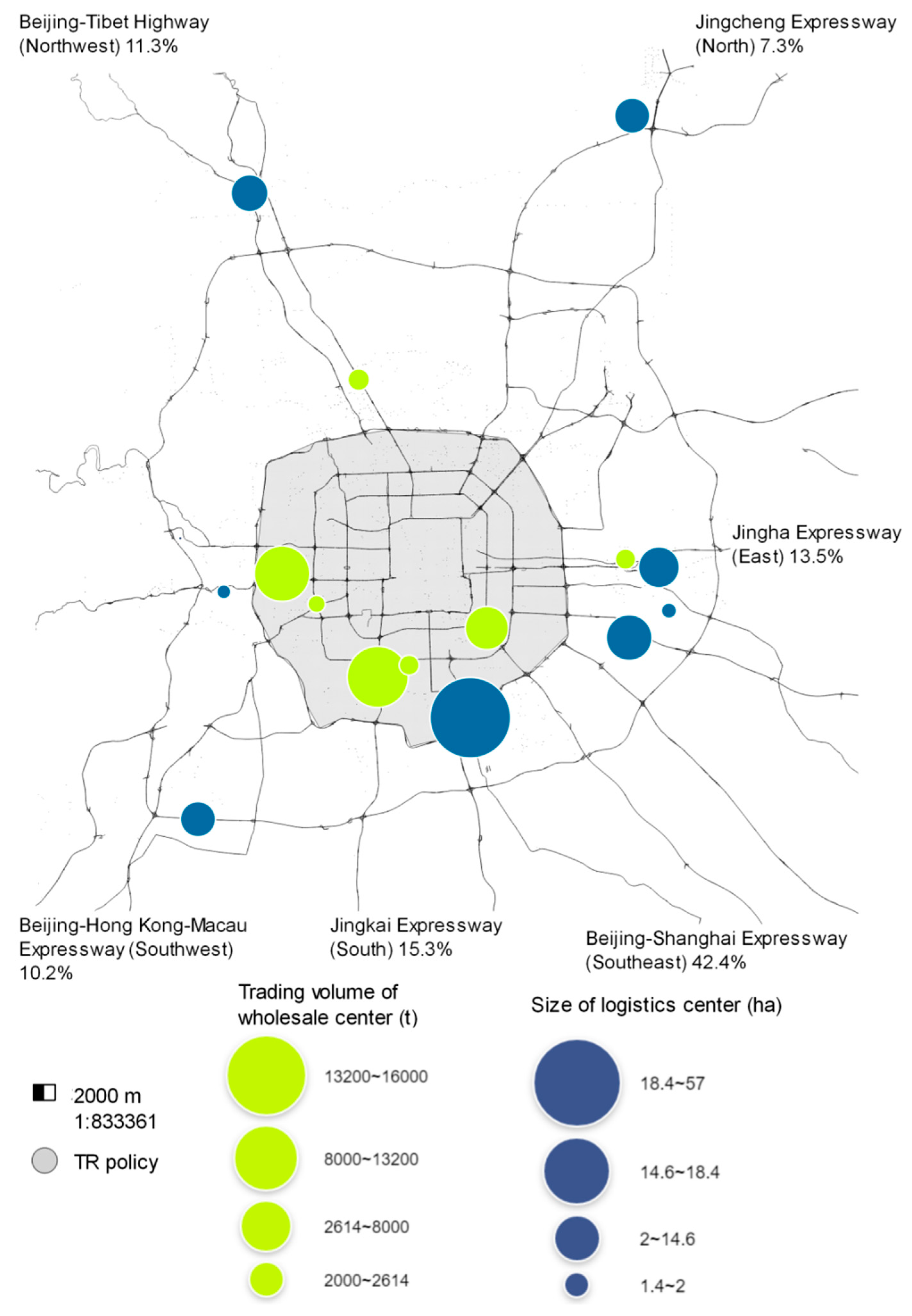
To solve all these problems above, we chose the case of Beijing agricultural freight, in which freight carriers suffer from both the time restriction and logistics sprawl policies. Specifically, for this case, the freight data is obtained based on surveys and the four-stage method; and the research method is the combination of traffic simulation and quantification models.

The contributions of this paper are as follows: (1) This paper explores the joint impact of two urban freight policies on the overall agricultural freight and environment. (2) The relationships between oil price, labor cost as well as load rate and the effectiveness of urban policies are further discussed.

The structure of this paper is as follows: In Section 2, we present the literature review. Section 3 introduces the case of Beijing agricultural freight. Section 4 explains the methodology of this paper, which includes scenario design, traffic simulation and quantitative models. Results are discussed in Section 5: We analyze the impact of urban freight policies and reflect on the relationships between different factors and policy effectiveness. Section 6 presents conclusions and policy implications.

2. Literature Review

This paper studies the impact of the time restriction and logistics sprawl policies through traffic simulation. Therefore, we summarize three aspects of literature: Time restriction, logistics sprawl and traffic simulation.

2.1. Time Restriction

Lots of scholars explored the time restriction policy by using different methodologies and cases. Quak and De Koster [13] examined the impact of time restrictions by measuring the freight performance of retailers. Research implied that public policies can affect the urban environment and freight costs of retailers, while logistical concepts, like network structure and logistics planning, determine the extent of time restriction’s impact. Nakamura et al. [14] analyzed the impact of the banned corridors in Osaka on traffic and emissions through macro-simulation. They found that this policy decreased the total travel time and emissions in the banned corridors, but increased on the total transportation network.

Gradually, researchers started to consider carriers’ responses. Quak and De Koster [15] took several cities in the Netherlands as examples to illustrate how to respond to urban policies by adjusting logistics concepts, like freight frequency, number of transit centers, vehicle type, unloading time, store hours, weekly volume and dispersion of stores (homogeneity). Stathopoulos et al. [16] also emphasized the importance of stakeholders’ reactions to urban freight policies. Afterwards, Lyons et al. [17] studied the impact of the time restriction policy on traffic congestion and local pollutant emissions, taking responses (like the changes of vehicle type, time schedule and delivery route) from carriers into consideration. By macro-simulation, they found that time restrictions increased gas pollutants in the restricted areas, but decreased emissions, travel time and vehicle kilometer trip (VKT) on all road networks. In addition to these studies, some researchers also used vehicle routing models to calculate the extra costs and distances resulting from time restrictions [18,19].

The above researchers have conducted substantial research on time restrictions. They believe that time restriction can lead to additional freight costs and pollutant emissions, while its actual effects are related to the freight carriers who might make adjustments in terms of vehicle type, time schedule, and delivery routes.

2.2. Logistics Sprawl

There are also substantial studies on logistics sprawl. The US Federal Highway Administration [20] believed that logistics sprawl increases delivery distance. Dablanc and Rakotonarivo [21] conducted the first empirical study on logistics sprawl using spatial center analysis. They found that the average distance from the logistics terminals to the barycenter increased from six km in 1974 to 16 km in 2008 and the total carbon dioxide emissions increased by 15,000 tons. Inspired by this study, more researchers used the same method to study the logistics sprawl in different cities, like Atlanta, Seattle, Los Angeles, Toronto and Paris, obtaining consistent results (e.g., [22,23,24]).

Most researchers believed that unreasonable relocation of logistics facilities led to unsustainable urban freight, like excessive congestion and greenhouse gas emissions [8], but some scholars question this view. Kohn and Brodin [25] considered that multimodal transport and delivery could effectively compensate for the negative environmental impact caused by additional driving distances. Sakai et al. [26] also proposed that the actual impact is determined by various factors including vehicle type, operational schedule, and origin and destination of goods.

These researchers have conducted substantial research logistics sprawl. Most researchers above believe that logistics sprawl can increase the burden of freight and environment, but few of them believe that some key factors, like vehicle type and operational schedule, can change the effects of logistics sprawl.

2.3. Traffic Simulation

In recent years, traffic simulation has become more and more popular in quantifying traffic policies and exploring traffic issues. In terms of time restriction and vehicle restrictions, Lyons et al. [17] quantified the time restriction policy by traffic simulation. Pu et al. [27] studied the impact of license plate restrictions on vehicle emissions in Hangzhou through the combination of traffic simulation (VISIM) and quantitative models (MOVES). The result demonstrated that this policy reduced the total vehicle kilometer trip (VKT) and the total emissions by 9.6% and 6.9%, respectively. In the areas of traffic congestion, Wu et al. [28] explored the problem of congestion charges in Beijing. By assuming different charging zone sizes, charging rates and transit service levels, the author constructed different scenarios, and then, carried out macro-simulation. The results indicated that congestion charges might increase the use of public transportation by 13% and reduce emissions. Similarly, Li and Huang [29] focused on how to alleviate the traffic congestion in the old areas of metropolis, providing an improved ant colony algorithm for the road transportation planning and using traffic simulation to prove its validity. Other issues, parking, road classification, crowd shipping, and freight demand management, also rely on the traffic simulation [30,31,32,33,34]. Therefore, because of the wide applicability of traffic simulation, we decided to adopt this method to study our research questions.

3. The Case of Beijing Agricultural Freight

3.1. Background Information

We choose the Beijing road network as our study area. Beijing, the capital of China, takes up an area of 16.41 million square kilometers and has a population of 21.71 million. This city implemented two policies to control freight activities. In 2017, the Beijing Municipal Government implemented the time restriction policy (TR policy) banning trucks over 3.5 t within the fifth ring from 6:00 a.m. to 11:00 p.m. [35]. Another adjustment is the logistics sprawl policy (LS policy), which requires that all large wholesale centers inside the fifth ring road of Beijing be replaced by new logistics centers outside the fifth ring road [7].

In Beijing, agricultural freight is based on a two-tier transportation system (See Figure 1). Agricultural products are firstly distributed to wholesale centers in Beijing (Stage 1) and then transported to each block (Stage 2) [36]. After implementing logistics sprawl, agricultural wholesale centers within the fifth ring are changed to the new logistics centers outside the fifth ring. Figure 1 presents the information of agricultural wholesale centers and new logistics centers in Beijing and the agricultural product flow into Beijing (obtained from the Beijing Municipal Commission of Commerce) [36]. In Figure 1, yellow and purple circles respectively reflect the geographical information of the wholesale centers and new logistics centers; their sizes indicate the transaction volumes of these centers (obtained from surveys with managers of seven large wholesales centers); and the metrics for the transaction volumes of wholesale centers and the size of new logistics centers are ton and hectare, respectively.

3.2. Data Derivation

To obtain the agricultural freight O-D matrices (vehicle trips for each origin-destination pair), we make the following simplifications. Firstly, we set the highway entrance of Beijing (near the sixth ring in Beijing) as the origin. Additionally, for statistical convenience, we treat each block as a point that includes all the agricultural demands of this block.

In fact, the state-preference survey for agricultural freight is time-consuming because local carriers consist of countless individuals and logistics enterprises. Therefore, we choose to derive the O-D matrix based on our surveys and a freight demand forecasting method. In terms of surveys, we interviewed the managers of seven major agricultural wholesale centers to figure out the transaction volume of agricultural products in Beijing. In terms of the freight demand forecasting method, we referred to the derivation process of Nuzzolo and Comi [37]. The specific derivation process is shown in Figure 2. Firstly, the quantity O-D matrices of agricultural products in Stage 1 (from Beijing entrance to wholesales center) are equal to the product of agricultural transaction volume of wholesale centers and the flow proportion of agricultural products into Beijing (See Figure 1). Since the wholesale centers have no obvious inclination to the supply source of agricultural products, we assume that the flow proportion into Beijing of each wholesale center’s agricultural product is in line with the overall situation. Secondly, the quantity O-D matrices of agricultural products in Stage 2 (from wholesales center to block) are deduced based on the agricultural supply (trading volume) and demand and the gravity model [38]. The demand for each block is derived from its population (whose information comes from National Bureau of Statistics) [39]; and the gravity model is the most common approach to construct O-D matrices based on supply and demand [40]. Thirdly, the vehicle O-D matrices (freight O-D matrices) are obtained in accordance with the quantity O-D matrices of agricultural products in Stage 1 and Stage 2, vehicle type (see

Table A1. Freight volume distribution (for different types of vehicles).

Research Time	Delivery Time Period	Vehicle Type	Delivery Stage (i)
			Stage1	Stage2
2011 (no urban freight policy)	Daytime	Standard trucks	100.00%	63.64%
	Night-time	Mini truck	0.00%	36.36%

Source: Obtained from managers of wholesales centers.

) and delivery time distribution (see

Table A2. Time period distribution.

Time Period	A	B	C
	Daytime Period 1: 6:00–9:00; 16:00–23:00	Daytime Period 2: 9:00–16:00	Night-Time: 23:00–6:00
Distribution	11.68%	69.66%	18.66%
Duration (hour)	10	7	7

Source: Du et al. [47].

), whose derivation process is totally presented in the Formula (1).

4. Methodology

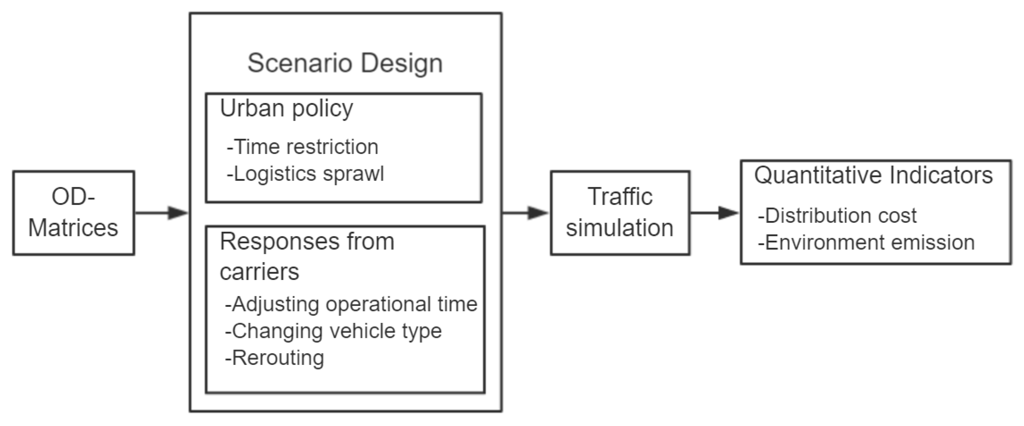
Our research framework is shown in Figure 3. The first step was to deduce the agricultural freight O-D matrices in Beijing. Then, we constructed several scenarios involved with different urban policies and responses from carriers (see Section 4) to adjust O-D matrices. Afterwards, we carried out macro-simulation for all scenarios and got simulation results. Finally, by quantitative models, we got the economic and environmental indicators. This section introduces the derivation of agricultural freight O-D matrices, the macro-simulation and quantitative models.

4.1. Scenario Design

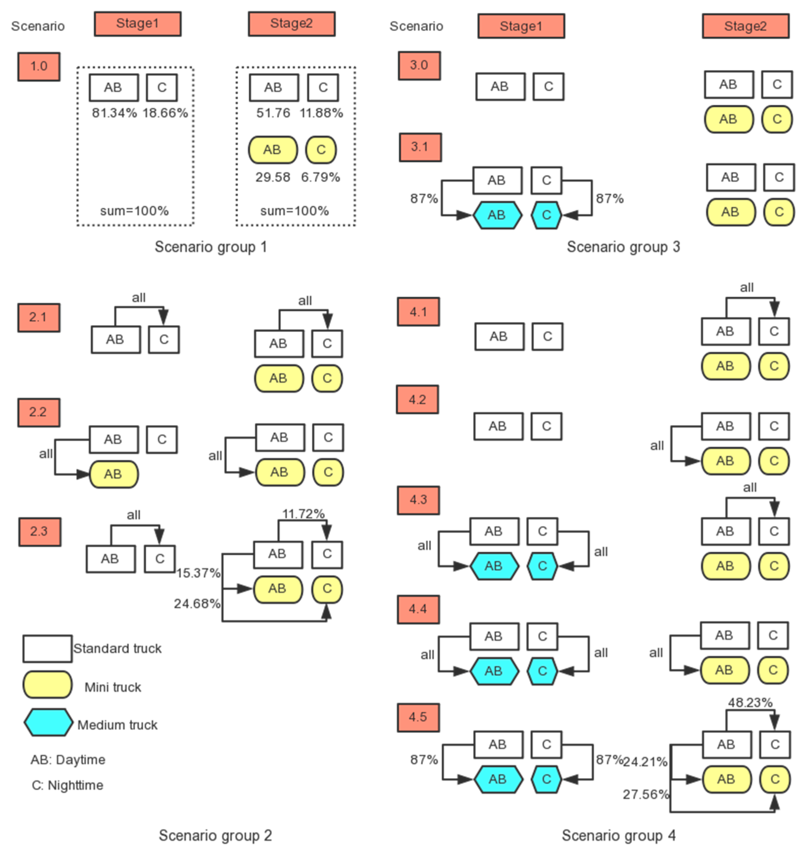
The implementation of policy is closely related to the responses from carriers. This chapter combines the policies (or combination of policies) and responses of carriers to construct four groups of scenarios (11 in total). Group 1 represents the base scenario; Group 2 embodies the time restriction policy; Group 3 reflects the logistics sprawl policy; and Group 4 embodies the joint implementation of two policies. Figure 4 presents the scenario design: The numbers below the boxes in scenario Group 1 embody the freight volume distribution at different stages in different time periods for different types of vehicles, which is derived from the freight volume distribution in 2011 (See Table A1) and time period distribution (See Table A2); the arrows in scenario groups 2–4 indicate the transfer of freight volume proportion in the aspects of operational schedule and vehicle, while the proportions adjacent to the arrows denote the transfer rates.

• Group 1 scenarios: Base scenario

Group 1 scenario embodies the urban agricultural freight in 2011 without restriction from urban policies, and it only includes scenario 1.0 (S1.0, S = scenario). In Stage 1, only standard trucks are used for distribution; in Stage 2, standard trucks are responsible for 63.6% of agricultural freight volume, while mini trucks are responsible for 36.4%.

To calculate freight O-D matrices, we set up the based O-D matrices. Before implementing the logistics sprawl policy, freight volume O-D matrices in Stage 1 and Stage 2 are OD₁ and OD₂, respectively; after the logistics sprawl, freight volume O-D matrices in Stage 1 and Stage 2 are OD₃ and OD₄, respectively. The O-D matrix of scenario n, in delivery stage i (including Stage 1 and Stage 2), at time period j (see Table A2), for vehicle k (see

Table 1. Major vehicle types and their parameters.

Size (k)	Abbreviation	Vehicle Type	Load Capacity
Mini truck	Mi	Changed from private cars, like Jinbei cars	2
Standard	St	Van	3.5
Medium	Me	Non-articulated truck (single unit)	10

), is $O{D}_{n,i,j,k}$.

$$O{D}_{n,i,j,k}=\frac{P_{n,i,j,k}}{D_j\ast L{c}_k\ast L{f}_k}O{D}_n$$

(1)

where, P_n,i,j,k is the proportion of agricultural freight volume of scenario n, in delivery stage i, at time period j, for vehicle k; D_j is the length of time period j; Lc_k and Lf_k respectively are the load capacity and the load rate of vehicle k.

• Group 2 scenarios: Time restriction (TR) policy and responses from carriers

Group 2 scenarios reflect the TR policy, involved with different reactions from carriers and changes from the base scenario. In S2.1 (S = scenario), standard trucks for daytime delivery are adjusted to night delivery. In S2.2, all standard trucks are replaced by mini trucks. And S2.3 embodies the realistic situation, and its modification refers to

Table A3. Responses from carriers.

Policies	Responses from Carriers
	Stage 1	Stage 2
TR policy	Standard trucks for daytime delivery change their schedule to night	Standard trucks are adjusted to other time period and other vehicle type; 23.60% of volume carried by standard trucks at night; 31.46% of freight volume carried by mini trucks at night; 44.94% of freight volume is delivered by mini trucks at daytime.
LS policy	13% of standard trucks for daytime delivery are replaced by medium trucks	No

. These adjustments of Group 2 scenarios are represented in Figure 4.

• Group 3 scenarios: Logistics sprawl (LS) policy

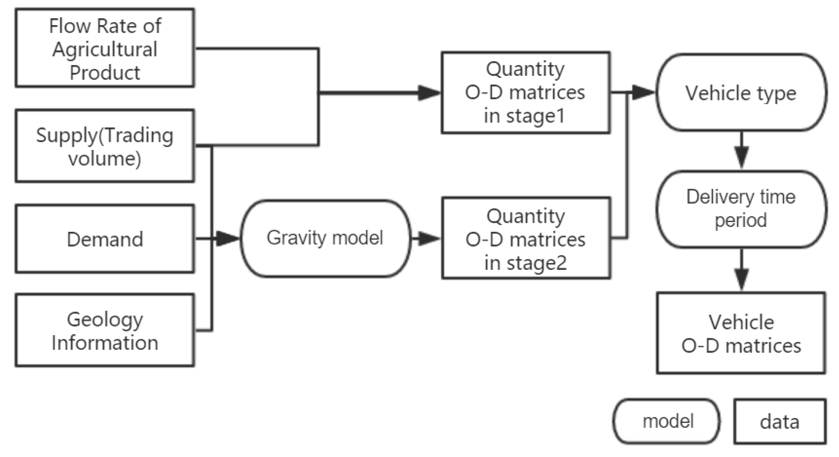
Group 3 scenarios represent the LS policy. It changes the distribution network because of the relocation of distribution centers. This paper assumes that the demand and supply of agricultural products do not change, and the scale of the new logistics center is proportional to the transfer volume. The O-D matrix is calculated by the same freight demand forecasting method (see Figure 2).

Scenario 3.0 reflects the changes of distribution network but does not consider the adjustments of carriers, whereas S3.1 (S = scenario) embodies both the modification of network and responses from carriers (see Table A3). These adjustments of group 3 scenarios are shown in Figure 4.

• Scenarios Group 4: TR and LS policies as well as responses from carriers

Group 4 scenarios combine the two policies (TR and LS policies) with all kinds of responses from freight carriers, and all the scenarios in group 4 are modified based on S3.0 (S = scenario). Scenario 4.1 is that standard trucks for daytime delivery in Stage 2 are changed to night delivery. Scenario 4.2 shows that standard trucks for daytime delivery in Stage 2 are replaced by mini trucks. In S4.3, standard trucks for daytime delivery in Stage 1 are replaced by medium trucks in Stage 1, and the delivery situation in Stage 2 is the same as that of S4.1. In S4.4, the distribution situation in stage1 is the same as that in S4.3, the distribution situation in Stage 2 is the same as that of S4.2. In addition, S4.5 represents the realistic situation (see Table A3). All the modifications of Group 4 scenarios are shown in Figure 4.

4.2. Traffic Simulation

Traffic simulation relies on the traffic simulator Aimsun supported by Transport Simulation System [41]. The inputs are the freight O-D matrices under different scenarios. Based on the simulation, we can obtain outputs, like total travel time, VKT and average speed, which can be used to calculate different indicators. The simulated background is shown as follows:

4.2.1. Vehicle Types

From our surveys in the seven large wholesale centers in Beijing, we found that there are many types of vehicles used for agricultural distribution. For the research convenience, we selected the most typical types of trucks (see Table 1). Additionally, according to the China Federation of Logistics and Purchasing [42], the average loading rate is 60%.

4.2.2. Urban Road Network

The road network is the urban area of Beijing. We downloaded the road network directly through Openstreetmap and imported it into the simulation software. To facilitate the simulation, we only retained the main road network and basic experimental interfaces. Moreover, we took the traffic congestion degree (referring to the traffic information provided by Beijing transport institute [43]) into account by setting different speed limits (See

Table 2. Average speed of road network in Beijing in different time periods.

Time Period		Average Speed (km/h)
Daytime off-peak hours	6:00–7:00; 9:00–17:00; 19:00–23:00	34.0
Daytime peak hours	7:00–9:00; 17:00–19:00	26.1
Nighttime	23:00–6:00	47.0

).

4.2.3. Model and Parameters

For our traffic simulation, the model of traffic route assignment was a C-logit model, which has been widely used in the lots of related studies. In all these studies, a necessary procedure is to adjust parameters to calibrate and validate the model because the fluctuation of parameters might lead to different results. The procedure of calibration and validation includes the following steps [44]: Index selection, data collection, parameter setting, initial evaluation, scenario construction, experimental simulation, parameter evaluation, and adjustment through the comparison of simulated index with realistic index.

In the paper, we firstly collected the traffic flow of the Beijing main road (including ring roads and highways) from different time periods and then conducted simulation by using the default models and parameters. The only modification is to set the highest average speed of Beijing as the limit of the road speed. Afterwards, we obtained the average speed through traffic simulation and compared this simulated speed with realistic speed (from Beijing transport institute [43]) by t-test (specific procedure can be found in Appendix B). Results (

Table A4. Significance test (t-test) for the realistic and simulated speed.

Time Period	Type of Speed	Average Speed	Number	Standard Deviation	Standard Error of the Mean	95% Confidence Interval (Lower and Upper)		T Value
Daytime (11:00–14:00)	Realistic	37.1706	18	1.44387	0.34032	−0.56045	1.32378	0.855
	Simulated	36.7889	18	0.83592	0.19703
Night-time (23:00–2:00)	Realistic	46.0096	18	3.82456	0.90146	−1.74271	2.07521	0.184
	Simulated	45.8433	18	0.19088	0.04499
Morning rush hour (7:00–9:00)	Realistic	28.2017	12	2.34165	0.67598	−0.73769	3.08446	1.351
	Simulated	27.0283	12	4.74161	1.36879
Evening rush hour (17:00–19:00)	Realistic	23.9865	12	0.97817	0.28237	−4.0957	−0.62637	−2.996
	Simulated	26.3475	12	3.30018	0.95268

) show that there is no obvious difference between the simulated speed and realistic speed, implying that the default parameters, like vehicle reaction time, road capacity, vehicle arrival distribution, can be used to reflect the realistic traffic situation of Beijing.

4.3. Quantitative Indicators

After getting the simulation outputs (time, distance and average time), we combined it with quantitative models to deduce the economic and environmental indicators.

Economic indicators referred to the urban freight costs (since we assume that the receivers’ willingness is totally reflected in the carriers’ operational changes, we do not consider the cost of receivers’ satisfaction). Though the composition of freight costs is very complicated, we only focused on variable freight costs, which are labor and fuel consumption costs.

Labor cost (LC) was equal to hourly wage multiplied by total travel time. The hourly trucker’s wage (See

Table 3. Trucker’s hourly wage (RMB).

	Mini and Standard Truck	Medium Truck
Daytime	30	45
Nighttime	42	63

) was obtained from the recruitment website (58.com [45]), while the total travel time was calculated by traffic simulation.

Fuel consumption cost (FCC) was calculated by multiplying fuel consumption by oil price. According to the government rules, only gasoline is allowed to be used in the urban areas of Beijing. The gasoline consumption is derived from CO₂ emissions, whose ratio to gasoline consumption is 2.7kg/1L [46]. According to the information of Beijing market, the price of gasoline is 7.3 RMB/L (obtained on 17 May 2018).

Therefore, the total cost (TC) is shown as follow:

$$\begin{array}{l}TC=LC+FCC\\ ={\displaystyle \sum _i^n{\displaystyle \sum _j^m{p}_{ij}{t}_{ij}}}+2.7\ast p_{oil}\ast E\end{array}$$

(2)

where,

• p_ij = hourly trucker’s wage for vehicle type i at the time period j
• t_ij = total travel time for vehicle type i at the time period j
• p_oil = oil price per literature (RMB)
• E = total carbon emission (L); 2.7 kg/L * E = total oil consumption (kg)
• n = number of vehicle types
• m = number of time period

Environmental Indicators

Environmental indicators refer to the gas emissions (CO, CO₂, NO_X, etc.) resulting from freight activities. Since CO₂ accounts for a large proportion of total emissions [46], we used it to reflect environmental indicators. The total amount of CO₂ emissions were equal to the carbon emission rate multiplied by VKT.

According to the MEET report of European Commission in 1999 [46], the CO₂ emissions rate is F(v) (kg/km) when speed is v.

$$F\left(v\right)=K+av+b{v}^2+c{v}^3+d\frac{1}{v}+e\frac{1}{v^2}+f\frac{1}{v^3} \left(\mathrm{Unit}\mathrm{kg}/\mathrm{km}\right)$$

(3)

These coefficients (K, a, …, f) differ per vehicle type. Therefore, we collected the information of the fuel consumption (to deduce carbon emissions) and the average speed from different drivers with different vehicles to obtain related parameters. Afterwards, we used these parameters to quantify simulation results.

Therefore, the total carbon emission E is shown as follows:

$$E={\displaystyle \sum _i^n{\displaystyle \sum _j^{m}F(v_{ij})\ast VK{T}_{ij}}}$$

(4)

where,

• VKT_ij = total vehicle kilometers trip of vehicle type i at the time period j (km)
• v_ij = average speed of vehicle type i at time period j (km/h)

5. Results and Discussion

5.1. Result Analysis

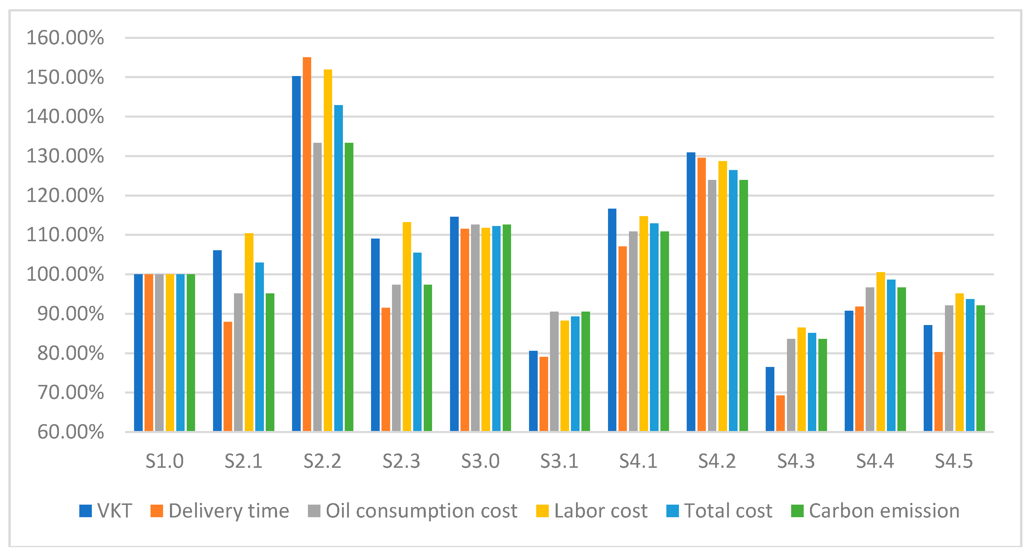
Results (see Figure 5) were obtained through the combination of traffic simulation and quantitative models. Different scenarios were compared with respect to travel time, vehicle kilometer trip (VKT), labor cost, fuel cost, total cost, and carbon emissions. Furthermore, we used the ratios of the total costs and carbon emissions of different scenarios to that of S1.0 to represent each policy’s economic and environmental effectiveness, respectively.

Group 2 scenarios embody the impact of TR policy. If carriers change their schedule to night (S2.1), the government can achieve their expected results and carriers can only increase their costs by 3.00%. In contrast, if carriers insist on daytime delivery by using mini trucks (due to the requirements of receivers, S2.2), TR policy can increase the freight costs and carbon emissions by 42.90% and 33.36%, respectively. Nevertheless, in reality, carriers generally make multiple instead of single adjustments. After taking all adjustments into account (S2.3), we find that TR policy can make only a few contributions to the environment (1.77% down) but raises a lot of costs (6.84% up).

Group 3 scenarios represent the effectiveness of LS policy. Though the logistics sprawl worsens the economic and environmental indicators, the responses from carriers can reverse the situation. Scenario 3.0 embodies that LS policy can increase the travel time and VKT, having negative impact on carriers and the environment. Nevertheless, LS policy allows the carriers in Stage 1 to replace standard trucks by medium trucks, which helps carriers improve their distribution efficiency (economic and environmental indicators decrease by 10.68% and 9.50%, respectively).

Group 4 scenarios reflect the joint implementation of two policies (the combined policies). Scenario 4.5 implies that the combined policies are beneficial to the economy (3.72% down) and environment (6.12% down) because the increased use of medium and standard trucks improves the distribution efficiency. Moreover, S4.3 shows that the combined policies allow the carriers to choose the optimal strategy to get the ideal economic and environmental indicators (decreased by 14.89% and 16.40%); Scenario 4.4 represents that, under the combined policies, even if carriers maintain daytime distribution, they still can lower their costs and emissions by adopting reasonable adjustment strategies.

The effectiveness of urban policies is closely involved with the responses from carriers because different responses from carriers may lead to different policy effects (like S2.1 vs. S2.2, S3.0 vs. S3.1, S4.1, S4.2 vs. S4.3, S4.4). More importantly, the responses from carriers are unexpected. For example, in S2.3, some freight carriers not only change the standard trucks to mini trucks but also adjust their schedule to night. Their changes seem to violate the market rules, because both the changes of vehicle type and modifications of operational schedule can increase costs and a single adjustment is enough to deal with TR policy. Two reasons can be used to explain this phenomenon: (1) Some receivers are influenced by TR policy and gradually change the receiving time from day to night, thereby forcing carriers to delivery at night; (2) TR policy shortens the time window for urban distribution and then reduces the single shipment, thus the usage of mini trucks increases.

5.2. The Impact of Other Factors on Policy Effectiveness

In the last chapter, we discussed the policy effectiveness based on background data (oil price, labor cost and load rate). However, these background data might change over time, so in this chapter, we explore the relationship between these factors and policy effectiveness from the economic perspective.

Policies’ economic effectiveness refers to the extent to which policies affect the urban freight costs. The effectiveness of TR policy, LS policy and the combined policies is reflected by the ratio of the total costs of S2.3, S3.1 and S4.5, respectively, to that of S1.0; and we use R2.3, R3.1 and R4.5 to represent their corresponding ratios. R > 1 indicates that the policy effectiveness is negative; R < 1 means that the policy effectiveness is positive; the smaller the ratio R is, the better the policy effectiveness is.

5.2.1. The Relationship between Oil Price and Labor Cost and Policy Effectiveness

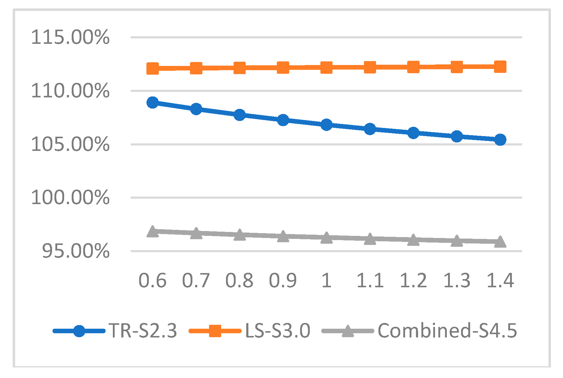
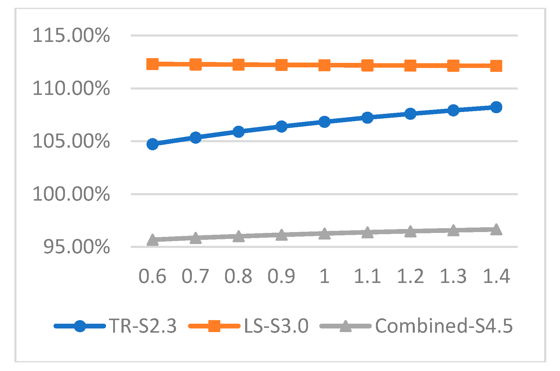
Figure 6 and Figure 7 indicate that the rise in oil prices weakens the negative impact of TR and increases the positive impact of combined policies, while the rise in trucker’s hourly wages worsens the negative effect of TR and attenuates the positive effect of the combined policies, all of which is due to the cost structure. Furthermore, the fluctuations of oil price and trucker’s hourly wage can only slightly influence the effectiveness of combined policies but largely influence that of the TR policy, thereby indicating that under combined policies, carriers are more likely to maintain the stability of their freight costs.

These phenomena are easy to understand: Since the fuel consumption costs of S2.3 and S4.5 account for a smaller proportion of total costs (compared with S1.0), the rise in oil price reduces their ratios “R2.3 and R4.5”, which means their policy in effect, becomes better (the smaller the ratio R is, the better the policy effectiveness is). Without doubt, the rise in oil price increases the urban freight costs of S1.0, S2.3, S3.0 and S4.5. However, the cost growth rate of S1.0 is higher than that of S2.3 and S4.5, which decreases R2.3 and R4.5. Similarly, since the labor costs of S2.3 and S4.5 account for a higher proportion of total costs, the rise in trucker’s hourly wages leads to a contrary trend in Figure 7.

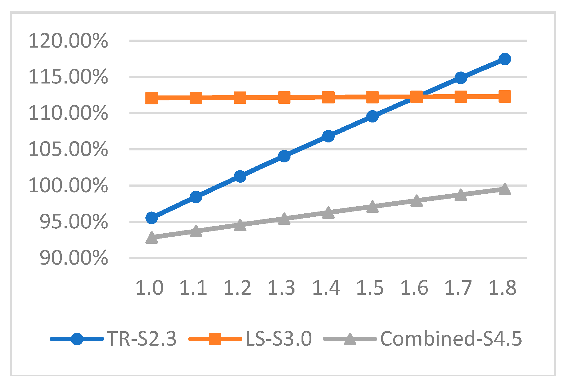
5.2.2. Night-to-Day Labor Cost Ratios and Policy Effectiveness

Night-to-day trucker’s wage ratio is a considerable factor because it fluctuates with the market and is related to the effectiveness of policies. The current night-to-day trucker’s wage ratio is 1.4, and the relationship between this ratio and the effectiveness of policies is presented in Figure 8. The increase in this ratio can both worsen the effectiveness of TR and combined policies, but it influences the TR policy more significantly. This indicates that under combined policies, freight carriers can lower their risk of cost fluctuations.

This phenomenon can be easily understood: TR and combined policies increase the nighttime delivery; hence, higher nighttime labor costs will lead to higher costs, which are reflected by the increase of R2.3 and R4.5.

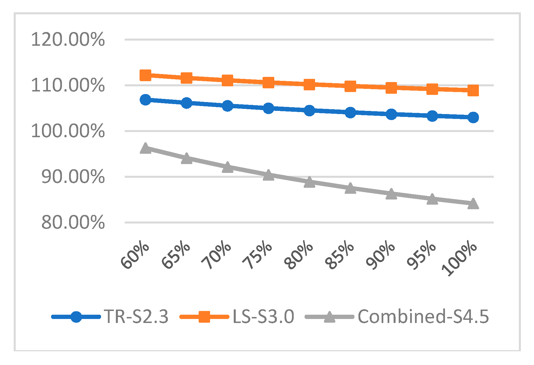
5.2.3. Load Rate and Policy Effectiveness

In Beijing, the load rate is maintained at 60% [42], but it might change over time. Figure 9 embodies the relationship between the load rate of mini truck and policies effectiveness. The increase of the load rate is beneficial to the effectiveness of all policies, but it contributes most to the effectiveness of combined policies.

The reasons for this are as follows: TR policy encourages the carriers to increase the usage of mini trucks; LS policy increases the delivery distance of mini trucks resulting from the logistics sprawl; and the combined policies increase both the delivery distance and usage of mini trucks.

6. Conclusions and Implications

This paper estimates the impact of time restriction and logistics sprawl on urban freight and the environment based on the case of Beijing agricultural freight by utilizing the combination of traffic simulation and quantitative models. Firstly, agricultural freight O-D matrices were derived from the supply and demand of agricultural products, gravity model and the distribution mode. Then, four groups of scenarios were constructed by combining different urban policies with responses from freight carriers and then these were used for simulation. Results show that though the time restriction and logistics sprawl policies are negative to carriers (6.84% and 12.20% up) and not significantly conducive to the environment (1.77% down and 12.62% up), their joint implementation can lower delivery costs (3.72%) and make contributions to the environment (6.12% down) because it prompts carriers to adopt appropriate operational strategies.

Taking responses from carriers into consideration is necessary because these responses are closely related to the policy implementation. Results indicate that the impact of time restriction on agricultural freight costs is negative, but its impact on the environment depends on whether carriers deliver at night. Additionally, though logistics sprawl can reduce the delivery efficiency (VKT and travel time increase by 14.59% and 11.56%, respectively) and generate additional carbon emissions (12.62%), it has positive impact on both carriers and the environment after considering the responses from carriers (costs and carbon emissions decrease by 10.68% and 9.50%, respectively).

Some factors, like oil price, labor cost, night-to-day labor cost ratio and load rate, can influence policy effectiveness (from the economic perspective). The rise in oil prices, the decline in labor costs, and the reduction in night-to-day labor cost ratio are all conducive to the effectiveness of TR policy and the combined policies. The increase in the load rate of mini trucks positively contributes to all the policy effectiveness but contributes the most to the combined policies. More importantly, under the combined policies, freight carriers are more likely to maintain the stability of their costs.

Policies for urban freight should consider the participation of different stakeholders involving aspects of economy, environment and society. For the case of Beijing, the combination of time restrictions and logistics sprawl would bring tremendous benefits to sustainability because all stakeholders such as freight carriers, local residents, and government agencies, can obtain benefits. Therefore, the combination of the two policies can be applied in other large cities. This research illustrates the effectiveness of policies and thus plays an important role in government decision-making.

References

1. Anderson, S.; Allen, J.; Browne, M. Urban logistics—How can it meet policy makers’ sustainability objectives? J. Transp. Geogr. 2005, 13, 71–81. [Google Scholar] [CrossRef]
2. Banister, D.; Stead, D.; Steen, P.; Akerman, J.; Dreborg, K.; Nijkamp, P.; Schleicher-Tappeser, R. European Transport Policy and Sustainable Mobility; Spon Press: London, UK, 2000. [Google Scholar]
3. Browne, M.; Allen, J. The impact of sustainability policies on urban freight transport and logistics systems. In Proceedings of the 8th World Conference Transport Research (WCTR), Antwerp, Belgium, 12–17 July 1998; Elsevier: Amsterdam, The Netherland; pp. 505–518. [Google Scholar]
4. Eren Akyol, D.; De Koster, R.B.M. Determining time windows in urban freight transport: A city cooperative approach. Transp. Res. Part E Logist. Transp. Rev. 2018, 118, 34–50. [Google Scholar] [CrossRef]
5. Dablanc, L.; Browne, M. Introduction to Special Section on Logistics Sprawl. Available online: https://www.sciencedirect.com/science/article/pii/S0966692319300158 (accessed on 25 March 2019).
6. He, M.; Shen, J.; Wu, X.; Luo, J. Logistics space: A literature review from the sustainability perspective. Sustainability 2018, 10, 2815. [Google Scholar] [CrossRef]
7. Beijing Municipal Commission of Commerce; Beijing Municipal Commission of Development and Reform. Beijing Logistics Industry Development Plan during the 13th Five-Year Plan Period (2016–2020). 2016. Available online: http://sww.beijing.gov.cn/zwxx/fzgh/ndgh/201607/t20160701_70597.html (accessed on 25 March 2019). (In Chinese)
8. Aljohani, K.; Thompson, R.G. Impacts of logistics sprawl on the urban environment and logistics: Taxonomy and review of literature. J. Transp. Geogr. 2016, 57, 255–263. [Google Scholar] [CrossRef]
9. Holguín-Veras, J.; Wang, X.; Sánchez-Díaz, I.; Campbell, S.; Hodge, S.D.; Jaller, M.; Wojtowicz, J. Fostering unassisted off-hour deliveries: The role of incentives. Transp. Res. Part A Policy Pract. 2017, 102, 172–187. [Google Scholar] [CrossRef]
10. Dablanc, L.; Rakotonarivo, D. The impacts of logistics sprawl: How does the location of parcel transport terminals affect the energy efficiency of goods’ movements in Paris and what can we do about it? Procedia Soc. Behav. Sci. 2010, 2, 6087–6096. [Google Scholar] [CrossRef]
11. Holguin-Veras, J.; Encarnacion, T.; Gonzalez-Calderon, C.A.; Winebrake, J.; Wang, C.; Kyle, S.; Herazo-Padilla, N.; Kalahasthi, L.; Adarme, W.; Cantillo, V.; et al. Direct impacts of off-hour deliveries on urban freight emissions. Transp. Res. Part. D Transport. Environ. 2018, 61, 84–103. [Google Scholar] [CrossRef]
12. Dell’olio, L.; Moura, J.L.; Ibeas, A.; Cordera, R.; Holguin-Veras, J. Receivers’ willingness-to-adopt novel urban goods distribution practices. Transp. Res. Part A Policy Pract. 2017, 102, 130–141. [Google Scholar] [CrossRef]
13. Quak, H.J.; de Koster, M.B.M. Exploring retailers’ sensitivity to local sustainability policies. J. Oper. Manag. 2007, 25, 1103–1122. [Google Scholar] [CrossRef]
14. Nakamura, Y.; Taniguchi, E.; Yamada, T.; Ando, N. A macroscopic traffic simulator for evaluating urban transport measures for heavy vehicles. Innov. City Logist. 2008, 1, 185–196. [Google Scholar]
15. Quak, H.J.; de Koster, M.B.M. Delivering Goods in Urban Areas: How to Deal with Urban Policy Restrictions and the Environment. Transp. Sci. 2009, 43, 211–227. [Google Scholar] [CrossRef]
16. Stathopoulos, A.; Valeri, E.; Marcucci, E. Stakeholder reactions to urban freight policy innovation. J. Transp. Geogr. 2012, 22, 34–45. [Google Scholar] [CrossRef]
17. Lyons, L.; Lozano, A.; Granados, F.; Guzmán, A. Impacts of time restriction on heavy truck corridors: The case study of Mexico City. Transp. Res. Part A Policy Pract. 2017, 102, 119–129. [Google Scholar] [CrossRef]
18. Munuzuri, J.; Grosso, R.; Cortes, P.; Guadix, J. Estimating the extra costs imposed on delivery vehicles using accesstime windows in a city. Comput. Environ. Urban Syts 2013, 41, 262–275. [Google Scholar] [CrossRef]
19. Munuzuri, J.; van Duin, R. Time constraints: the cost of sustainability. In Sustainable Urban Logistics: Concepts, Methods and Information Systems; Gonzalez-Feliu, J., Routhier, J.-L., Semet, F., Eds.; Springer: Berlin, Germany, 2014; pp. 165–185. [Google Scholar]
20. Federal Highway Administration. FHWA Freight and Land Use Handbook; US Department of Transport: Washington, DC, USA, 2012. Available online: http://ops.fhwa.dot.gov/publications/fhwahop12006/fhwahop12006.pdf (accessed on 25 March 2019).
21. Dablanc, L.; Ross, C. Atlanta: A mega logistics center in the Piedmont Atlantic Megaregion (PAM). J. Transp. Geogr. 2012, 24, 432–442. [Google Scholar] [CrossRef]
22. Dablanc, L.; Ogilvie, S.; Goodchild, A. Logistics Sprawl. Transp. Res. Rec. J. Transp. Res. Board 2014, 2410, 105–112. [Google Scholar] [CrossRef] [Green Version]
23. Woudsma, C.; Jakubicek, P.; Dablanc, L. Logistics Sprawl in North America: Methodological Issues and a Case Study in Toronto. Transport. Res. Procedia 2016, 12, 474–488. [Google Scholar] [CrossRef] [Green Version]
24. Heitz, A.; Dablanc, L. Logistics Spatial Patterns in Paris. Transp. Res. Rec. J. Transp. Res. Board 2015, 2477, 76–84. [Google Scholar] [CrossRef]
25. Kohn, C.; Brodin, M.H. Centralised distribution systems and the environment: how increased transport work can decrease the environmental impact of logistics. Int. J. Logist. Appl. 2008, 11, 229–245. [Google Scholar] [CrossRef]
26. Sakai, T.; Kawamura, K.; Hyodo, T. Locational dynamics of logistics facilities: Evidence from Tokyo. J. Transp. Geogr. 2015, 46, 10–19. [Google Scholar] [CrossRef]
27. Pu, Y.; Yang, C.; Liu, H.; Chen, Z.; Chen, A. Impact of license plate restriction policy on emission reduction in Hangzhou using a bottom-up approach. Transp. Res. Part D Transp. Environ. 2015, 34, 281–292. [Google Scholar] [CrossRef]
28. Wu, K.; Chen, Y.; Ma, J.; Bai, S.; Tang, X. Traffic and emissions impact of congestion charging in the central Beijing urban area: A simulation analysis. Transp. Res. Part D Transp. Environ. 2017, 51, 203–215. [Google Scholar] [CrossRef]
29. Li, Z.; Huang, J. How to mitigate traffic congestion based on improved ant colony algorithm: A case study of a congested old area of a metropolis. Sustainability 2019, 11, 1140. [Google Scholar] [CrossRef]
30. Lopez, C.; Zhao, C.L.; Magniol, S.; Chiabaut, N.; Leclercq, L. Microscopic simulation of cruising for parking of trucks as a measure to manage Freight Loading Zone. Sustainability 2019, 11, 1276. [Google Scholar] [CrossRef]
31. Li, Y.; Bao, L.; Li, W.; Deng, H. Inventory and policy reduction potential of greenhouse gas and pollutant emissions of road transportation industry in China. Sustainability 2016, 8, 1218. [Google Scholar] [CrossRef]
32. Gatta, V.; Marcucci, E.; Nigro, M.; Patella, S.M.; Serafini, S. Public transport-based crowdshipping for sustainable city logistics: Assessing economic and environmental impacts. Sustainability 2018, 11, 145. [Google Scholar] [CrossRef]
33. Schulte, J.; Ny, H. Electric road systems: Strategic stepping stone on the way towards sustainable freight transport? Sustainability 2018, 10, 1148. [Google Scholar] [CrossRef]
34. Holguín-Veras, J.; Sánchez-Díaz, I. Freight Demand Management and the Potential of Receiver-Led Consolidation programs. Transp. Res. Part A Policy Pract. 2016, 84, 109–130. [Google Scholar] [CrossRef]
35. Beijing Municipal Commission of Transport; Beijing Municipal Environmental Protection Bureau; Beijing Traffic Management Bureau. Notice on Traffic Management Measures for Partial Cargo Vehicles to Reduce Pollutant Emissions. 2017. Available online: http://www.bjepb.gov.cn/bjhrb/index/qwfb/818274/index.html (accessed on 25 March 2019). (In Chinese)
36. Beijing Municipal Commission of Commerce. Development Plan of Agricultural Products Circulation System in Beijing during the 12th Five-Year Plan Period (2011–2015). 2012. Available online: http://zfxxgk.beijing.gov.cn/110020/zzqgh33/2012-01/18/content_291114.shtml (accessed on 25 March 2019). (In Chinese)
37. Nuzzolo, A.; Comi, A. Urban freight demand forecasting: A mixed quantity/delivery/vehicle-based model. Transp. Res. Part E Logist. Transp. Rev. 2014, 65, 84–98. [Google Scholar] [CrossRef]
38. Chen, S.; Wen, D.U.; Gao, S. The study on the model and parameter of urban-trip distribution in metropolises of China. Syst. Eng. 2002, 20, 63–66. (In Chinese) [Google Scholar]
39. National Bureau of Statistics. Beijing’s Sixth National Census in 2010. 2010. Available online: http://www.stats.gov.cn/tjsj/tjgb/rkpcgb/dfrkpcgb/201202/t20120228_30381.html (accessed on 25 March 2019). (In Chinese)
40. Grange, L.D.; Troncoso, R.; Ibeas, A.; González, F. Gravity model estimation with proxy variables and the impact of endogeneity on transportation planning. Transp. Res. Part A Policy Pract. 2009, 43, 105–116. [Google Scholar] [CrossRef]
41. Transport Simulation Systems. Aimsun 8 Dynamic Simulators Users’ Manual. Available online: https://www.scribd.com/document/266245543/Aimsun-Users-Manual-v8 (accessed on 30 June 2019).
42. China Federation of Logistics & Purchasing. Analysis of China’s Intelligent Logistics Status: Empty-Loading Rate Reaches 40%. 2016. Available online: http://www.stats.gov.cn/tjsj/tjgb/rkpcgb/dfrkpcgb/201202/t20120228_30381.html (accessed on 25 March 2019). (In Chinese)
43. Beijing Transport Institute. Annual Report on Beijing’s Traffic Development. 2018. Available online: http://www.bjtrc.org.cn/JGJS.aspx?id=5.2&Menu=GZCG (accessed on 25 March 2019). (In Chinese).
44. Zhang, W.; Lu, J.; Xu, P.; Zhang, Y. Moving towards sustainability: Road grades and on-road emissions of heavy-duty vehicles—A case study. Sustainability 2015, 7, 12644–12671. [Google Scholar] [CrossRef]
45. 58.com. Recruitment Information for Truckers. 2018. Available online: https://www.58.com/daichepeisong/ (accessed on 25 March 2019). (In Chinese).
46. Jabali, O.; Van Woensel, T.; de Kok, A.G. Analysis of Travel Times and CO2 Emissions in Time-Dependent Vehicle Routing. Prod. Oper. Manag. 2012, 21, 1060–1074. [Google Scholar] [CrossRef]
47. Caijun, D.U.; Liu, C.; Chen, J. Urban freight demand survey research taking Beijing as an example. J. Chongqing Jiaotong Univ. 2014, 14, 21–24. (In Chinese) [Google Scholar]
Figure 1. The implementation of time restriction and logistics sprawl in Beijing.
Sustainability 11 03675 g001
Figure 2. Agricultural freight O-D matrices derivation process.
Sustainability 11 03675 g002
Figure 3. Research framework.
Sustainability 11 03675 g003
Figure 4. Scenario design.
Sustainability 11 03675 g004
Figure 5. Economic and environmental indicators. (Supplementary notes: the percentages are the ratios of the indicators of different scenarios to that of S1.0).
Sustainability 11 03675 g005
Figure 6. Relationship between oil prices and effectiveness of policies.
Sustainability 11 03675 g006
Figure 7. Relationship between trucker’s hourly wage and effectiveness of policies.
Sustainability 11 03675 g007
Figure 8. Relationship between night-to-day trucker’s wage ratio and effectiveness of policies.
Sustainability 11 03675 g008
Figure 9. Relationship between the load rate of mini truck and effectiveness of policies.
Sustainability 11 03675 g009