Distribution Network Power Loss Analysis Considering Uncertainties in Distributed Generations

Abstract

Distribution network loss analysis is crucial for the economic operation in residential distribution networks. The increasing level of distributed generation (DG) has considerably improved the overall sustainability but raised the uncertainty in system losses and exacerbated voltage profiles. This paper presents a nodal distribution loss analysis approach in which the losses induced by loads and DGs are calculated recursively. In order to characterize the uncertainty, the Latin hypercube sampling (LHS)-based approach is presented for obtaining DG output samples. Further, the LHS-based sampling and loss analysis methods are combined into a proposed stochastic framework for loss analysis, which takes into account the DG output uncertainty. Case studies on a 36-bus radial distribution network verified the stochastic loss analysis method. Compared with the simple random sampling method, the proposed LHS-based stochastic loss analysis method can reach the same accuracy level for nodal voltages and losses more efficiently.

1. Introduction

1.1. Background and Motivation

As the electric power industry become more and more deregulated, changes are taking place in the power distribution network for retail power delivery. Distributed generations (DGs), controllable loads and the demand response (DR) programs are being integrated into the active distribution networks (ADN), which provide better controllability and higher efficiency. An essential issue for ADN is to quantify the power losses associated with generators and loads so that the network efficiency can be evaluated and the operations can be optimized.

DGs in the distribution network is composed of various, controllable and non-controllable energy sources. For example, roof-top solar panels and small-scale wind generators are uncontrollable generations which depend on the availability of solar irradiance and wind speed, respectively. Although controllable energy sources, including household energy storage systems and gasoline generators, are typically used in complementary with the non-controllable sources, the power output of DGs is still subject to high uncertainty, which may significantly affect the distribution loss analysis.

1.2. Literature Review

The existing work in distribution loss analysis traces back to transmission network loss analysis. Proposed methods in the literature include

• Prorated (pro rata, PR) method which distributes the losses based on the actual power consumption of devices, regardless of network configuration and the load locations [1]. The PR method is simple to implement but unfair for loads that are near the generation sources. In other words, loads that are remote from the generations should have accounted for more losses, which is not considered in the PR method.
• Distance-adjusted pro rata (DAPR) method. The distance of the load to a root node, such as a generation source, along with the power demand, are considered as a megawatt-mile factor [2]. The DAPR method includes the distance factor but does not consider the nonlinear characteristics of the power flow.
• Incremental loss method. By using the linearization in the Newton–Raphson method for solving the power flow, the incremental losses can be derived by perturbing the loads or generations with a small value [3,4,5,6]. This method assumes a single slack bus or distributed slack buses and can cause over-calculation of total losses since the slack bus is not included in the iterations. Another disadvantage of this method is the unsuitability for ADN, which has a high R/X ratio.
• Network analysis based methods. This type of methods calculates the losses based on the network impedance or admittance matrix [7]. Methods in this category include the Z-bus method [8], the modified Y-bus method [9], branch-current decomposition method [10], and the succinct method [11].
• Power tracing methods. This type methods traces the losses based on branch power flow and the connected nodal injections. Existing traceing methods include graph theory-based tracing methods as proposed in [12,13] and various tracing algorithms [14,15,16,17]. Normalization is required if the method overestimates or underestimates the total losses.

A comprehensive review of the loss allocation methods can be found in [18]. To adopt and apply the above-mentioned methods for radial distribution systems with DGs [19], which create multiple points of sources, considerations must be given for (a) the radial topology of the distribution networks; (b) the characteristics of the net generation nodes (power sources) and the net load nodes (power sinks); and (c) the uncertainty of the output of DGs. This paper adopts a fair nodal power tracing method [20], which takes into account the network topology and does not assign losses to the pure power sources.

In terms of the uncertainty of DG outputs, the existing literature on stochastic analysis can be summarized as follows.

• Monte–Carlo based simple random sampling (SRS) method. This method first takes a large number of random samples for each group of random variables. If the number of samples is large enough, according to the large number theory, the samples could represent the random variables. Next, calculations are performed over each group of the random variables, and the results are analyzed to obtain the statistics.
• Monte–Carlo based reduced sampling methods. Different from the simple random sampling, these methods use more sophisticated sampling techniques, such as layered sampling, to reduce the redundancy of samples and thus reduce the computational burden [21].

There is existing literature that studies the distribution network power flow problem and analyzes the losses in a probabilistic or stochastic framework. Literature [22,23,24,25,26] studied the three-phase power flow problem with uncertainty considering DGs using neural networks, and literature [27,28,29] considered droop-based controls with stochastic load and generation characteristics in the power flow formulation. Literature [30] proposed a sensitivity-based model for low-voltage distribution systems with DGs. Some literature studied the distribution network reconfiguration problem [31] with stochastic characteristics of electric vehicles and DGs in the objective of loss minimization [32]. Literature [33] studied the problem of allocating DG resource consider the stochastic features. To the knowledge of the authors, there is currently no existing literature on analyzing the distribution network loss considering the stochastic characteristics of DG outputs.

The distribution network loss analysis method discussed in this paper is not a power flow calculation method. Instead, it is a loss allocation method that takes the power flow solution and allocates the losses to associated nodes (generations and loads). In particular, this paper adopts the voltage correction power flow method to solve for bus voltages, generator reactive power, branch power flows, and slack bus power injections. Power flow solutions using any particular power flow solution methods can be used and adapted in the stochastic framework for loss analysis.

1.3. Contribution and Paper Organization

In this paper, the Latin hypercube sampling method is proposed for linearized distribution network loss analysis in order to consider the uncertainty of DGs. The main contributions of this paper are:

• Presenting a nodal power loss tracing method for quantifying the losses induced by DGs in the distribution network. The presented model is linear and thus rapid to calculate for large data samples.
• Proposing a Latin hypercube sampling backed stochastic loss analysis method that is applicable for representing the uncertainty of DG power outputs. The sampling method is first introduced, and the procedure to evaluate the samples are elaborated.

This paper is organized as follows: Section 1 gives an overview of the topic and introduces the state of the arts in distribution network loss tracing and uncertainty handling. Section 2 presents the nodal loss tracing method for distribution loss assessment. Section 3 presents the methodology for the Latin Hypercube Sampling method for reducing the sample sizes in the Monte–Carlo simulations. Section 4 proposes the stochastic distribution loss evaluation and elaborates the procedure for integrating the stochastic variables into the loss analysis model. Section 5 presents case studies and discussions in a modified 36-bus system and compares the LHS-based method with the SRS-based method. Finally, Section 6 draws the conclusions.

2. Distribution Network Loss Assessment

2.1. Basic Formulations for Loss Assessment

Consider a radial distribution network with distribution lines and nodes, where DGs and loads can be connected. One of the nodes is used to connect the distribution network to the transmission system. First, the following assumptions are made for assigning the network losses:

• The loss assigned to the node connecting the distribution to the transmission networks is zero. This node is responsible for balancing the power supply and demand but does not account for any loss caused by power distribution.
• The loss assigned to the load on the nodes where the net generation is positive, namely, the total power generation is greater than the total load, is considered as zero. The load on such nodes are fully supplied locally and will not incur any distribution loss.

More generally, let a distribution line i–k with the impedance $Z_{ik}=R_{ik}+j{X}_{ik}$ connect two nodes, i and k, where the DG on node i sends power to the load on node k, the active power loss $L_{ik}$ on this line can be given as

$$L_{ik}=I_{ik}^2{R}_{ik}=\frac{P_{ik}^2+Q_{ik}^2}{|V_i{|}^2}{R}_{ik}=c(P_{ik}^2+Q_{ik}^2),$$

(1)

where $P_{ik}$ and $Q_{ik}$ are the active and reactive power sending from i to k through the line; $V_i$ is the nodal voltage at node i; the loss coefficient $c=R_{ik}/{|V_i|}^2$. The two terms in (1) corresponds to the active power loss due to sending active power and reactive power, respectively.

Consider two loads on the receiving end k with apparent power of $S_{load,k1}$ and $S_{load,k2}$, given as

$$S_{load,k1}=P_{load,k1}+j{Q}_{load,k1},$$

(2)

$$S_{load,k2}=P_{load,k2}+j{Q}_{load,k2}.$$

(3)

Take the transmitted active power for example, but also note that the following deductions apply to the reactive power related losses, $P_{ik}$ can be expressed in terms of $P_{load,k1}$ and $P_{load,k2}$ as

$$P_{ik}=P_{load,k1}+P_{load,k2}+L_{ik}$$

(4)

Denote the first term in (1) $c{P}_{ik}^2$ as $L_{p,ik}$ and the second term $c{Q}_{ik}^2$ as $L_{q,ik}$. Therefore, the active power loss due to transmitting active power from i to k can be expressed as

$$L_{p,ik}=c{P}_{ik}^2=c{(P_{load,k1}+P_{load,k2}+L_{p,ik})}^2,$$

(5)

where $L_{p,ik}$ is the portion of active power loss between line i–k caused by acitve power transmission, which is denoted by the p in the subscript. In most cases, the active power loss $P_{loss,ik}$ can be ignored because it is usually small compared with $P_{load,k1}$ + $P_{load,k2}$. Equation (5) can be simplified into

$$L_{p,ik}\approx c{(P_{load,k1}+P_{load,k2})}^2.$$

(6)

Comparing Equations (5) and (6), the condition for the approximation to satisfy can be deduced as (7)

$$0=c{L}_{p,ik}[L_{p,ik}+2(P_{load,k1}+P_{load,k2})].$$

(7)

The solution to this condition is that the losses on the line, $L_{p,ik}$, is small enough. Although this may be true for some nodes, such a condition might not hold for the whole system. This approximation is more of an engineering practice than strict mathematical deduction. Other approaches, such as Taylor expansion, may be employed to obtain linear approximations of (5).

Equation (6) indicates that both the loads $k1$ and $k2$ contribute to the losses collectively. Next, the losses are distributed based on the Shapley value in the cooperative game theory. The losses assigned to load $k1$ is related to the load level of both $k1$ itself and the other loads, in this case, $k2$. Using the Shapley value formulation, the right-hand side of (6) can be expressed as

$$L_{p,ik}=c{P}_{ik}^2=c(P_{load,k1}^2+P_{load,k1}{P}_{load,k2})+c(P_{load,k2}^2+P_{load,k1}{P}_{load,k2}),$$

(8)

where on the right-hand side, the first term is the loss due to serving the active power load of $k1$, and the second term corresponds to that of $k2$. This formulation can be extended to the case with n loads for node k. For example, the losses assigned to load k–j, $j=1,\dots ,n$, can be calculated using

$$L_{p,kj}=c{P}_{load,kj}\sum _{m=1}^n{P}_{load,km}.$$

(9)

2.2. Assessing Load-Induced Distribution Losses

Load-induced distribution losses are defined as the power losses caused by serving load in the distribution network. This subsection derives the formulations to assess the active power loss, but the reactive power losses can be assessed using a similar approach. For an arbitrary node i that connects to node k and a set of nodes M, the total active power load on node i consists of (a) the active power flow $P_{ik}$ through line ik; (b) the active power flow through the set of lines, i–j, $j\in M$; and (c) the local active power load set L on node n.

Denote the total power losses due to active power transmission occurred in the system as $L_{p,i}$, according to Shapley value theory in Equation (6), the total amount of losses correspond to a total portion of

$${(\sum _{j\in M}{P}_{ij}+\sum _{l\in L}{P}_{load,il})}^2.$$

(10)

Using Equation (8) the portion of losses associated with the branch flow $P_{ik}$ is

$$P_{ik}(\sum _{j\in M}{P}_{ij}+\sum _{l\in L}{P}_{load,il}).$$

(11)

Therefore, using (10) and (11), the amount of losses associated with $P_{ik}$ is given as

$$L_{p,ik}=L_{p,i}^{load}\frac{P_{ik}}{{\sum }_{j\in M}{P}_{ij}+{\sum }_{l\in L}{P}_{load,il}},$$

(12)

which is derived by dividing $P_{loss,j}$ based on the portion of the branch losses in the total portions. Similar to (12), the share of losses of the load l at node i is given as

$$L_{p,il}^{load}=L_{p,i}^{load}\frac{P_{load,il}}{{\sum }_{j\in M}{P}_{ij}+{\sum }_{l\in L}{P}_{load,il}},$$

(13)

which indicates that the larger the load, the more losses it bears for the power delivery.

For node k, the total losses can be iteratively computed by summing up the assigned losses from the connected node set n and the branch losses i–k, $i\in \mathit{n}$. The formulation for the losses assigned to node k is given as

$$L_{p,k}^{load}=\sum _{i\in n}(L_{p,i}^{load}\frac{P_{ik}}{{\sum }_{j\in M}{P}_{ij}+{\sum }_{l\in L}{P}_{load,il}}+L_{p,ik}).$$

(14)

In Equation (14), the two terms in the summation on the right-hand side are (a) the share by node k of the total losses on node i; and (b) the branch losses i–k, assuming a power flow direction from i to k.

The same procedure can be applied to derive the portion of the power losses caused by transmitting reactive power, $L_{q,ik}^{load}$ and $L_{q,k}^{load}$, and therefore obtain the total losses $L_k^{load}$, $k=1,\dots ,n$. Note that the total losses calculated here need to be normalized to eliminate the overestimation.

2.3. Assessing DG-Induced Power Distribution Losses

On the other hand, if a node is connected to DG and is supplying power to other nodes, it is responsible for a portion of the losses at the nodes that receive power from it. The DG-induced power distribution losses are used to quantify the total losses a DG should be responsible for. Note that the major difference between the load-induced losses and DG-induced losses is the power flow direction.

For node k with a set of G DGs connected, the active power loss assigned to DG $g\in \mathit{G}$ can be calculated as

$$L_{p,kg}^{gen}=L_{p,k}^{gen}\frac{P_{gen,kg}}{{\sum }_{j\in M}{P}_{kj}+{\sum }_{g\in G}{P}_{gen,kg}},$$

(15)

where M is the set of nodes that receive power from node k. Summing up all the losses associated with supplying the loads that are connected to node k, the total DG-induced loss is expressed as

$$L_{p,k}^{gen}=\sum _{i\in \mathit{n}}(L_{p,i}^{gen}\frac{P_{gen,ig}}{{\sum }_{j\in M}{P}_{ij}+{\sum }_{g\in G}{P}_{gen,ig}}+L_{p,ik}),$$

(16)

which has the same structure of Equation (14) but differs in the first term, namely, instead of counting in the share of load-induced losses, the DG-induced losses are considered in (16).

The same procedure is applicable to obtain the portion of power losses associated with supplying reactive power, namely, $L_{q,kg}^{gen}$ and $L_{q,k}^{gen}$. By summing up $L_{p,k}^{gen}$ and $L_{q,k}^{gen}$, the total losses assigned to node k for supplying power can be obtained as $L_k^{gen}$, where $k=1,\dots ,n$. Similarly, $L_k^{gen}$ needs to be normalized.

2.4. Normalization

As previously mentioned, the calculated total power losses associated with load and DG need to be normalized to avoid overestimation. Based on the assumption that the total actual losses are fully assigned to all the loads and DGs, the following equations can be used normalize the load-induced losses and DG-induced losses into the dimension of power:

$$L_{i,norm}^{load}=P_{loss,total}\frac{L_i^{load}}{\sum L_i^{load}+\sum L_k^{gen}},$$

(17)

$$L_{k,norm}^{gen}=P_{loss,total}\frac{L_k^{gen}}{\sum L_i^{load}+\sum L_k^{gen}}.$$

(18)

Equations (17) and (18) provide the final losses associated with the loads on node i and the DGs on node k.

2.5. Procedure for Calculating Distribution Losses

The overall procedure for calculating active power distribution losses induced by load or DG are summarized as follows:

• Initialization: Based on the assumption, set the losses to zeros for the node that connects the distribution network to the transmission network, alongside the nodes that are purely power sources (for calculating load-induced losses) or purely power demands (for calculating DG-induced losses).
• Recursive calculation: For each of the rest nodes, recursively calculate the losses on the nodes that send power to (for calculating load-induced losses) or receive power from (for calculating DG-induced losses) the current node, and then calculate the losses on the current node using (14) (for load-induced losses) or (16) (for DG-induced losses).
• Normalize the load-induced and DG-induced losses using the equations in Section 2.4.

3. Latin Hypercube Sampling Approach

The LHS approach consists of two major steps: sampling and combination. The sampling process involves generating samples from known patterns to represent the probability distribution of the variables. The combination process involves permuting and combining the samples from the first step to achieve a higher level of variable independence. The sampling and combination process are described in following subsections.

3.1. Sampling Process

Before looking into the mathematical details, it is crucial to note that the LHS is essentially a layered sampling method for each variable in the input variable vector. Assume K inputs for the problem, and the random variables are $x_1$, $x_2$, …, $x_K$. For each random variable, a cumulative probability distribution (CDF) function exist in the general formulation

$$y_k=C_k(x_k),k=1,\dots ,K$$

(19)

where $C_k$ is the cumulative distribution function, and $y_k$ is the value of the CDF at the given point. Apparently, $y_k\in [0,1]$.

To obtain N samples for the k-th variable in the input vector, the steps are given as follows and shown in Figure 1.

• Evenly divide the range of [0, 1] into N intervals, each with a probability range of $1/N$.
• Take one sample randomly from each interval. A total of N cumulative probability values, $y_{k1},\dots ,y_{kN},$ are obtained in this step.
• Calculate the corresponding variable value for each sample by using the inverse CDF function, namely, $x_{kn}=C_k^{-1}(y_{kn})$.

Repeat the steps above for all the variables in the input vector to obtain a $K\times N$ input matrix $S_0$ where the rows are the independent random variables, and the columns are different samples.

3.2. Permutation and Combination Processes

The values in the input matrix $S_0$ are ordered for each variable. The purpose of combination and permutation is to reduce the correlation between the variables through reordering. Existing permutation methods include random permutation, heuristics based methods, optimization-based methods, and Cholesky decomposition based methods. Although sophisticated permutation and combination methods yield better data samples, the computational burden for permutation may be heavy.

In this paper, the random permutation method is chosen as a simple yet effective approach. The advantages of the random permutation include the simplicity of implementation and the efficiency of execution. The random permutation is carried out using the following steps:

• Generate a linear space matrix L having the same shape of S. Each row in the L matrix is a linear space with an increment of 1, namely, $1,\dots ,N$.
• For each row in L, permute the elements in a random order. Effective implementation is to loop over the row back and forth, for each element, randomly choose another element and randomly decide whether to swap.
• For each row in the $S_0$ matrix, reorder the elements based on the index order in the permutated L matrix to obtain the permutated sampling matrix S.

The LHS-based sampling method has the following characteristics compared with the SRS-based method:

• Using LHS, the number of samples for each variable can be controlled to a manageable size of N, which can be adjustable based on the distribution characteristics. On the other hand, the number of samples for the LHS must be determined before running the case studies, but the SRS-based method allows for building up the cases incrementally.
• The LHS-based method guarantees (one and only one) sampling coverage for each interval. The SRS-based on method, however, requires a considerably larger sample size to cover the range.
• For linear problems, the LHS-based methods can provide an estimation for the output, which is a linear weighted combination of the inputs.

4. Stochastic Distribution Network Loss Analysis

4.1. General Formulation and Solution Work Flow

This section discusses the generalities for applying the LHS-family based sampling methods to the proposed distribution network loss evaluation model. The input-output relationship of a general distribution network power flow problem is given as

$$\mathit{y}=g(\mathit{x})$$

(20)

$$\mathit{L}=h(\mathit{y}),$$

(21)

where in (20), x contains the inputs vector of the generation power injections, $P_g$ and $Q_g$, and load power consumption, $P_g$ and $Q_d$, g is the set of power flow equations describing the nodal power balancing, $y$ is the output vector that contains the voltage magnitude V and voltage phasor $\theta$. In (21), h is the set of equations to compute the losses based on the loss calculation method presented in Section 2, yielding losses L for each generation-load pairs.

In stochastic loss analysis methods, the input variable array $x$ is substituted with sampled values using random sampling or the proposed LHS methods. The input variables are assumed to be independent. The output variables, $y$ and $L$, are statistically observed for all the input samples. In our case, the input array consists of the random DG output power and random load power, while the output array consists of the nodal voltages and losses.

The workflow of solving the proposed model is given as follows:

• Load the network data file that includes bus and branch parameters, base generation and load data, and shunt admittance data.
• Determine and set sample size N for each input variable.
• Using the selected sampling method (random or LHS), generate the input data matrix S with the size of $K\times N$, where K is the number of input variables.
• For each array of input sample, namely, each column in S, run the network loss evaluation routine and store the output data accordingly.
• After all the sample inputs are computed, compute the statistics (mean value and standard deviation) of the output data for each variable.

Note that in Step 3, the appropriate sampling method, either simple random sampling or LHS-family based sampling, should be used. Results from the simple random sampling are treated as the benchmark data for verifying the proposed LHS-based method. The number of samples used in the random sampling should be at least one order of magnitude higher than that for the LHS-based methods.

4.2. Statistical Metrics for the Stochastic Method

Statistical metrics can provide quantitative assessment of the proposed stochastic approach. In this paper, the error ratios for the mean and standard deviation are adopted. This metric calculates the error ratios of the proposed LHS-based method in relative to the simple random sampling method.

$${ϵ}_{mean}=|\frac{{\mu }_{y,SRS}-{\mu }_{y,LHS}}{{\mu }_{y,SRS}}|$$

(22)

$${ϵ}_{std}=|\frac{{\sigma }_{y,SRS}-{\sigma }_{y,LHS}}{{\sigma }_{y,SRS}}|,$$

(23)

where, in (22) and (23), $\mu$ and $\sigma$ are the mean value and standard deviation, the subscript SRS corresponds to the simple random sampling, and y represents the output variables including voltage magnitude, voltage phase angle, and generator-load losses. Finally, the average error is defined by taking the arithmetic mean of all errors to quantify the performance of the LHS-based method for all samples.

5. Discussion and Case Studies

The proposed LHS-based distribution network loss analysis method has been applied to a 36-bus test system for verification. Case studies are performed in MATLAB R2018b on a PC with Intel i7-4770 and 8 GB of RAM.

The 36-Bus Radial System

The 36-bus distribution network data is available at [20], and its single-line diagram is shown in Figure 2. The test system consists of 35 branches and three DGs, located on buses 34, 35, and 36, still importing power from other buses. The outputs of the three DGs are 240 kW + 96 kVar, 400 kW + 160 kVar, and 400 kW + 160 kvar, respectively. A total of six active power and reactive power variables considered as random for the loss analysis problem. The DG outputs are sampled between 0.5 to 1.5 pu for all cases. The power flow calculation results of the base case is shown in

Table 1. Initial power flow solutions of the 36-bus radial test system in the base distributed generation (DG) scenario.

Bus	Pl (kW)	Ql (kW)	Qsh (kVar)	Pg (kW)	Qg (kVar)	V (pu)	$\mathit{\theta }$ (deg)
1	0	0	0	2765.022	1856.322	1	0
2	100	60	0	0	0	0.998	0.015
3	90	40	0	0	0	0.988	0.097
4	120	80	0	0	0	0.984	0.163
5	60	30	0	0	0	0.980	0.230
6	60	20	0	0	0	0.970	0.260
7	200	100	0	0	0	0.968	0.176
8	200	100	0	0	0	0.967	0.203
9	60	20	0	0	0	0.964	0.192
10	60	20	0	0	0	0.962	0.191
11	45	30	0	0	0	0.962	0.197
12	60	35	0	0	0	0.961	0.206
13	60	35	0	0	0	0.960	0.220
14	120	80	0	0	0	0.960	0.229
15	60	10	0	0	0	0.961	0.243
16	60	20	0	0	0	0.962	0.266
17	60	20	0	0	0	0.965	0.390
18	90	40	0	0	0	0.967	0.429
19	90	40	0	0	0	0.997	0.004
20	90	40	0	0	0	0.994	−0.063
21	90	40	0	0	0	0.993	−0.082
22	90	40	0	0	0	0.992	−0.103
23	90	50	0	0	0	0.985	0.067
24	420	200	0	0	0	0.978	−0.021
25	420	200	0	0	0	0.975	−0.064
26	60	25	0	0	0	0.969	0.292
27	60	25	0	0	0	0.967	0.338
28	60	20	0	0	0	0.961	0.451
29	120	70	0	0	0	0.956	0.549
30	200	600	0	0	0	0.954	0.635
31	150	70	0	0	0	0.955	0.604
32	210	100	0	0	0	0.955	0.606
33	60	40	0	0	0	0.957	0.645
34	0	0	0	240	96	0.972	0.914
35	0	0	0	400	160	0.994	3.005
36	0	0	0	400	294.341	1	3.04
Total	3715	2300	0	3805.022	2406.663	-	-

, and the initial loss analysis results are given in

Table 2. Active power and reactive power losses associated with the loads and DGs.

	Active Power Losses (kW)				Reactive Power Losses (kVar)
Bus/Gen	1	34	35	36	1	34	35	36
2	0.229	0	0	0	0.103	0	0	0
3	1.141	0	0	0	0.322	0	0	0
4	2.179	0	0	0	0.951	0	0	0
5	1.343	0	0	0	0.365	0	0	0
6	1.946	0	0	0	0.337	0	0	0
7	6.846	0	0	0	2.631	0	0	0
8	3.673	0.087	0	0	1.893	1.413	0	0
9	1.163	0.151	0	0	0.386	0.433	0	0
10	1.235	0.22	0	0	0.418	0.45	0	0
11	0.969	0.108	0	0	0.709	0.39	0	0
12	1.297	0.179	0	0	0.818	0.502	0	0
13	1.253	0.191	0.137	0	0.844	0.483	0.203	0
14	0.089	−0.137	1.778	0	0.92	0.136	7.62	0
15	0	0	1.515	0	0	0	3.328	0
16	0	0	0.956	0	0	0	3.612	0
17	0	0	0.824	0	0	0	3.41	0
18	0	0	0.627	0	0	0	5.261	0
19	0.243	0	0	0	0.101	0	0	0
20	0.521	0	0	0	0.351	0	0	0
21	0.571	0	0	0	0.41	0	0	0
22	0.615	0	0	0	0.468	0	0	0
23	1.462	0	0	0	0.673	0	0	0
24	9.363	0	0	0	4.653	0	0	0
25	10.665	0	0	0	5.672	0	0	0
26	2.058	0	0	0	0.487	0	0	0
27	2.174	0	0	0	0.476	0	0	0
28	2.617	0	0	0	0.326	0	0	0
29	6.212	0	0	0	2.012	0	0	0
30	15.902	0	0	−2.445	23.693	0	0	2.549
31	1.229	0	0	2.691	−0.272	0	0	8.786
32	0	0	0	5.227	0	0	0	13.945
33	0	0	0	0.919	0	0	0	4.398
34	0	0	0	0	0	0	0	0
35	0	0	0	0	0	0	0	0
36	0	0	0	0	0	0	0	0

.

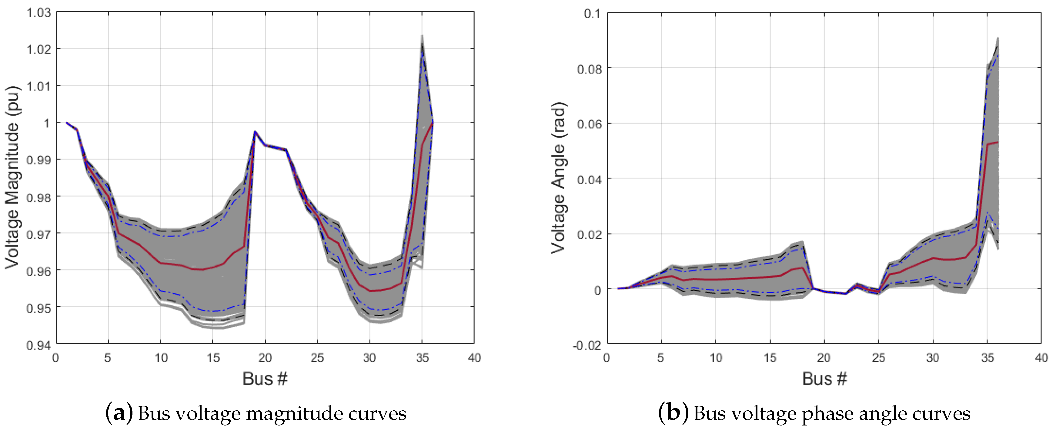
First, the bus voltage and power loss results of the stochastic loss analysis are presented. As a benchmark, the simple randomly sampled input consisted of 50,000 samples, while the LHS-family based method contained 300 samples. Figure 3 shows the bus voltage magnitude and voltage phasor curves, including both LHS-based sampling data (shown in grey) and the average results of 50,000 uniformly sampled data (shown in red). Figure 4 and Figure 5 shows the active power and reactive power losses assigned to buses 1, 34, 35 and 36 due to serving loads on other buses. It can be observed that

• The losses associated with the DG on bus 1 and the loads on buses with DGs were zero.
• Losses due to active power and reactive power for the buses with DGs that were exporting power were not affected by the stochastic inputs. Buses that were farther from the DGs and the substation (bus 1) were subject to higher loss variation under uncertain DG outputs.
• The voltages on the buses close to the substation (bus 1) had comparatively small variations. This applies to buses 2, 3, 19, 20, 21 and 22.
• The difference of the 85% and the 95% confidence intervals for voltages from the SRS and LHS, shown in Figure 3, are within 10⁻³ per unit.

The calculation listed in

Table 3. Voltage magnitude and angle differences between the averages from Latin hypercube sampling (LHS) and simple random sampling (SRS).

Bus	1	2	3	4	5	6	7	8	9
V (×10−4 pu)	0	0.001	0.007	0.011	0.015	0.022	0.020	0.018	0.023
$\theta$ (×10−4 deg)	0	0.017	0.011	0.018	0.025	0.045	0.044	0.044	0.046
Bus	10	11	12	13	14	15	16	17	18
V (×10−4 pu)	0.029	0.030	0.032	0.039	0.043	0.046	0.049	0.057	0.061
$\theta$ (×10−4 deg)	0.049	0.049	0.049	0.053	0.055	0.057	0.058	0.064	0.066
Bus	19	20	21	22	23	24	25	26	27
V (×10−4 pu)	0.001	0.001	0.001	0.001	0.007	0.007	0.007	0.025	0.029
$\theta$ (×10−4 deg)	0.002	0.002	0.002	0.002	0.002	0.011	0.011	0.049	0.054
Bus	28	29	30	31	32	33	34	35	36
V (×10−4 pu)	0.041	0.051	0.059	0.069	0.072	0.074	−0.004	0.102	0
$\theta$ (×10−4 deg)	0.082	0.104	0.113	0.142	0.152	0.166	−0.014	0.131	0.562

also shows that the differences between the average voltage magnitude from the SRS and LHS are within 10⁻⁴ per unit, which is a small value to prove the validity of using LHS to reduce the sampling size while obtaining similar results.

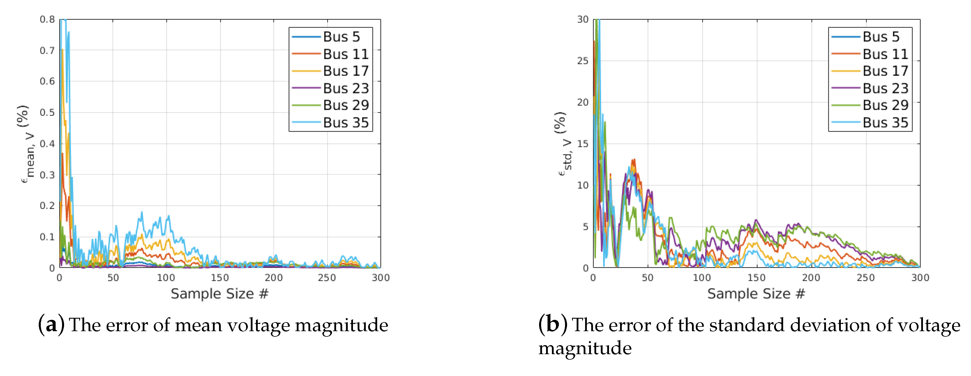
Next, the mean and standard deviation error metrics were compared to assess the performance of random sampling and the LHS-based sampling using Equations (22) and (23). Figure 6 and Figure 7 shows the error metrics of the mean value and the standard deviation of the bus voltages. Note that the horizontal axis is the total number of samples that are used to calculate the metrics. For example, if the sample size $N=200$, the results calculated using the first 200 samples are utilized to compute the metrics and yield one point in each curve.

From the error curves of the voltage mean and standard deviation, the following were observed for this test case:

• The mean values from both random sampling and LHS-based sampling approached the SRS results after about 150 samples.
• The standard deviations started at a high level and fluctuated with a downward trend as the number of samples increased.

The error curves of the active power loss mean and standard deviations were also compared. The two curves in each subfigure of Figure 8 and Figure 9 correspond to the losses caused by supplying power from the DG on bus 1 to the loads on Bus 31 and 32, respectively. Comparing Figure 8 and Figure 9, the following observations made:

• The results of the random sampling had higher fluctuations in the error metrics compared with the results of the LHS-based methods.
• The LHS-based method converged to the benchmark value faster, as seen in the error of the mean value plots in Figure 9a.
• Due to the completely random feature, the errors of the standard deviation did not show a consistent decrease as the number of samples increased, as seen in Figure 8b. The decreasing trend was more consistent using the LHS-based sample inputs.

6. Conclusions

This paper presents a novel stochastic loss analysis approach for distribution systems based on Latin hypercube sampling. The presented loss analysis approach calculates the losses for the distribution nodes recursively, based on the connected load and the power flow on the connected lines. The LHS-based approach generates samples for the stochastic DG output more efficiently by using layered sampling and permutation techniques, compared with the SRS-based method. The following conclusions are drawn for the proposed LHS-based stochastic distribution loss analysis method:

• The distribution loss analysis method can account for the network topology and the amount of load and can assign losses for both loads and DGs.
• The stochastic analysis verifies that, for the same amount of load, the more losses it occurs, the farther it is from the substation bus.
• The LHS can achieve the same level of errors in the mean value and standard deviation with significantly fewer samples, compared with the SRS-based sampling method.

Future work on the stochastic distribution network losses includes minimizing the voltage profile deviation caused by the stochastic nature of DGs and considering the correlations between the DGs.

References

- Conejo, A.J.; Arroyo, J.M.; Alguacil, N.; Guijarro, A.L. Transmission Loss Allocation: A Comparison of Different Practical Algorithms. IEEE Trans. Power Syst. 2002, 17, 571–576. [Google Scholar] [CrossRef]
- Happ, H.H. Cost of wheeling methodologies. IEEE Trans. Power Syst. 1994, 9, 147–156. [Google Scholar] [CrossRef]
- Mutale, J.; Strbac, G.; Curcic, S.; Jenkins, N. Allocation of losses in distribution systems with embedded generation. IEE Proc. Gen. Transm. Distrib. 2000, 147, 7–14. [Google Scholar] [CrossRef]
- Galiana, F.D.; Conejo, A.J.; Kockar, I. Incremental transmission loss allocation under pool dispatch. IEEE Trans. Power Syst. 2002, 17, 26–33. [Google Scholar] [CrossRef]
- Carpaneto, E.; Chicco, G.; Sumaili Akilimali, J. Loss partitioning and loss allocation in three-phase radial distribution systems with distributed generation. IEEE Trans. Power Syst. 2008, 23, 1039–1049. [Google Scholar] [CrossRef]
- Carpaneto, E.; Chicco, G.; Sumaili Akilimali, J. Characterization of the loss allocation techniques for radial systems with distributed generation. Electr. Power Syst. Res. 2008, 78, 1396–1406. [Google Scholar] [CrossRef]
- Atanasovski, M.; Taleski, R. Energy summation method for loss allocation in radial distribution networks with DG. IEEE Trans. Power Syst. 2012, 27, 1433–1440. [Google Scholar] [CrossRef]
- Conejo, A.J.; Galiana, F.D.; Kockar, I. Z-bus loss allocation. IEEE Trans. Power Syst. 2001, 21, 54. [Google Scholar] [CrossRef]
- Daniel, J.; Salgado, R.; Irving, M. Transmission loss allocation through a modified Ybus. IEE Proc. Gen. Transm. Distrib. 2005, 152, 208–241. [Google Scholar] [CrossRef]
- Carpaneto, E.; Chicco, G.; Akilimali, J.S. Branch current decomposition method for loss allocation in radial distribution systems with distributed generation. IEEE Trans. Power Syst. 2006, 21, 1170–1179. [Google Scholar] [CrossRef]
- Fang, W.L.; Ngan, H.W. Succinct method for allocation of network losses. IEE Proc. Gen. Transm. Distrib. 2002, 149, 171–174. [Google Scholar] [CrossRef]
- Strbac, G.; Kirschen, D.; Ahmed, S. Allocating transmission system usage on the basis of traceable contributions of generators and loads to flows. IEEE Trans. Power Syst. 1998, 13, 527–534. [Google Scholar] [CrossRef]
- Lim, V.S.; McDonald, J.D.; Saha, T.K. Development of a new loss allocation method for a hybrid electricity market using graph theory. Electr. Power Syst. Res. 2009, 79, 301–310. [Google Scholar] [CrossRef]
- Costa, P.M.; Matos, M.A. Loss Allocation in Distribution Networks With Embedded Generation. IEEE Trans. Power Syst. 2004, 19, 384–389. [Google Scholar] [CrossRef]
- Rao, M.S.S.; Soman, S.A.; Chitkara, P.; Gajbhiye, R.K.; Hemachandra, N.; Menezes, B.L. Min-max fair power flow tracing for transmission system usage cost allocation: A large system perspective. IEEE Trans. Power Syst. 2010, 25, 1457–1468. [Google Scholar] [CrossRef]
- Savier, J.S.; Das, D. An exact method for loss allocation in radial distribution systems. Int. J. Electr. Power Energy Syst. 2012, 36, 100–106. [Google Scholar] [CrossRef]
- Jagtap, K.M.; Khatod, D.K. Loss allocation in radial distribution networks with various distributed generation and load models. Int. J. Electr. Power Energy Syst. 2016, 75, 173–186. [Google Scholar] [CrossRef]
- Kalambe, S.; Agnihotri, G. Loss minimization techniques used in distribution network: Bibliographical survey. Renew. Sustain. Energy Rev. 2014, 29, 184–200. [Google Scholar] [CrossRef]
- Expoßsito, A.G.; Santos, J.M.R.; Garcißa, T.G.; Ruiz Velasco, E.A. Fair allocation of transmission power losses. IEEE Trans. Power Syst. 2000, 15, 184–188. [Google Scholar] [CrossRef]
- Ghofrani-Jahromi, Z.; Mahmoodzadeh, Z.; Ehsan, M. Distribution Loss Allocation for Radial Systems Including DGs. IEEE Trans. Power Deliv. 2014, 29, 72–88. [Google Scholar] [CrossRef]
- Yu, H.; Chung, C.Y.; Wong, K.P.; Lee, H.W.; Zhang, J.H. Probabilistic load flow evaluation with hybrid latin hypercube sampling and cholesky decomposition. IEEE Trans. Power Syst. 2009, 24, 661–667. [Google Scholar] [CrossRef]
- Baghaee, H.R.; Mirsalim, M.; Gharehpetian, G.B.; Talebi, H.A. Three-phase AC/DC power-flow for balanced/unbalanced microgrids including wind/solar, droop-controlled and electronically-coupled distributed energy resources using radial basis function neural networks. IET Power Electron. 2016, 10, 313–328. [Google Scholar] [CrossRef]
- Baghaee, H.R.; Mirsalim, M.; Gharehpetian, G.B.; Talebi, H.A. Application of RBF neural networks and unscented transformation in probabilistic power-flow of microgrids including correlated wind/PV units and plug-in hybrid electric vehicles. Simul. Model. Pract. Theory 2017, 72, 51–68. [Google Scholar] [CrossRef]
- Baghaee, H.R.; Mirsalim, M.; Gharehpetian, G.B.; Talebi, H.A. Fuzzy unscented transform for uncertainty quantification of correlated wind/PV microgrids: possibilistic–probabilistic power flow based on RBFNNs. IET Renew. Power Gen. 2017, 11, 867–877. [Google Scholar] [CrossRef]
- Baghaee, H.R.; Mirsalim, M.; Gharehpetian, G.B.; Talebi, H.A. Generalized three phase robust load-flow for radial and meshed power systems with and without uncertainty in energy resources using dynamic radial basis functions neural networks. J. Clean. Prod. 2018, 174, 96–113. [Google Scholar] [CrossRef]
- Baghaee, H.R.; Mirsalim, M.; Gharehpetan, G.B.; Talebi, H.A. Nonlinear load sharing and voltage compensation of microgrids based on harmonic power-flow calculations using radial basis function neural networks. IEEE Syst. J. 2018, 12, 2749–2759. [Google Scholar] [CrossRef]
- Baghaee, H.R.; Mirsalim, M.; Gharehpetian, G.B. Performance Improvement of Multi-DER Microgrid for Small- and Large-Signal Disturbances and Nonlinear Loads: Novel Complementary Control Loop and Fuzzy Controller in a Hierarchical Droop-Based Control Scheme. IEEE Syst. J. 2018, 12, 444–451. [Google Scholar] [CrossRef]
- Baghaee, H.; Mirsalim, M.; Gharehpetian, G.; Talebi, H. Eigenvalue, Robustness and Time Delay Analysis of Hierarchical Control Scheme in Multi-DER Microgrid to Enhance Small/Large-Signal Stability Using Complementary Loop and Fuzzy Logic Controller. J. Circuits Syst. Comput. 2017, 26, 1–34. [Google Scholar] [CrossRef]
- Baghaee, H.R.; Mirsalim, M.; Gharehpetian, G.B. Power Calculation Using RBF Neural Networks to Improve Power Sharing of Hierarchical Control Scheme in Multi-DER Microgrids. IEEE J. Emerg. Sel. Top. Power Electron. 2016, 4, 1217–1225. [Google Scholar] [CrossRef]
- Di Fazio, A.R.; Russo, M.; Valeri, S.; De Santis, M. Sensitivity-based model of low voltage distribution systems with distributed energy resources. Energies 2016, 9, 801. [Google Scholar] [CrossRef]
- Savier, J.S.; Das, D. Impact of network reconfiguration on loss allocation of radial distribution systems. IEEE Trans. Power Deliv. 2007, 22, 2473–2480. [Google Scholar] [CrossRef]
- Cui, H.; Li, F.; Fang, X.; Long, R. Distribution network reconfiguration with aggregated electric vehicle charging strategy. In Proceedings of the IEEE Power and Energy Society General Meeting, Denver, CO, USA, 26–30 July 2015. [Google Scholar] [CrossRef]
- Mahmoud, K.; Yorino, N.; Ahmed, A. Optimal Distributed Generation Allocation in Distribution Systems for Loss Minimization. IEEE Trans. Power Syst. 2016, 31, 960–969. [Google Scholar] [CrossRef]
Figure 1.
Latin hypercube sampling from a cumulative distribution function.
Figure 2.
Single-line diagram of the 36-bus radial test system.
Figure 3.
Bus voltage phasors: comparison of the results of the LHS-based samples and the average results of the random samples. The grey curves are solutions of the LHS-based samples, and the red curve is the average of 50,000 randomly sampled data. The black dash curves correspond to the 95% confidence interval; and the blue dot-dash curves are the bounds of the 85% confidence interval.
Figure 4.
Active power losses for the buses connected to substation and DGs.
Figure 5.
Reactive power losses for the buses connected to substation and DGs.
Figure 6.
In the simple random sampling, the error metrics of the mean values and standard deviations of the bus voltages as the number of samples increase. Only the first 300 samples out of 50,000 are shown.
Figure 7.
In the Latin hypercube sampling (LHS)-based approach, the error metrics of the mean values and standard deviations of the bus voltages as the number of samples increase.
Figure 8.
In the random sampling method, the error metrics of the mean values and standard deviations of the active power losses as the number of samples increase.
Figure 9.
In the LHS-based sampling sampling, the error metrics of the mean values and standard deviations of the active power losses as the number of samples increase.