Quality Recovery or Low-End Recovery? Profitability and Environmental Impact of Durable Product Recovery


1
School of Management and Economics, Beijing Institute of Technology, Beijing 100081, China
2
School of Economics and Management, University of Shanxi, Taiyuan 030006, China
*
Author to whom correspondence should be addressed.
Sustainability 2019, 11(6), 1726; https://doi.org/10.3390/su11061726
Submission received: 23 February 2019
/
Revised: 16 March 2019
/
Accepted: 16 March 2019
/
Published: 21 March 2019
(This article belongs to the Special Issue How Better Decision-Making Helps to Improve Sustainability - Part II)
Abstract
:With the rising awareness of environmental responsibility in industrial production, a series of recovery strategies have been developed and play different roles in achieving sustainability. In this study, we examine when quality recovery, low-end recovery, and hybrid recovery result in a win-win outcome where both profitability and environmental performance can be improved for a durable product manufacturer. We develop a game-theoretic model to analyze the manufacturer’s payoffs under different recovery strategies. A secondary market where used products can be resold among consumers is also considered. We obtain the results by comparing the profitability and environmental impact under each recovery strategy. Hybrid recovery causes both synergy and a contradiction effect between quality and low-end recovery. It always improves the win-win outcome of low-end recovery and it can also improve the win-win outcome of quality recovery under a high recovery standard when the recovered value is not too high. The technology improvement only achieves environmental sustainability under sufficient stringent recovery standard, otherwise, it may backfire and deteriorate the environment. We offer insights for the policymaker to understand the role of the recovery standard in achieving the win-win outcome and the importance of setting a proper recovery standard in achieving environmental sustainability.
1. Introduction
The growth of industrial production and over-consumption caused by humans is intensifying the resource shortage and environmental burden of waste. With the rising awareness of environmental responsibility in industrial production, product reuse has been widely accepted as a green strategy to alleviate these crises [1,2]. Product recovery is a general term of product reuse, through which the after-use product is collected and processed by firms in an environmentally friendly manner. This process keeps a product (or part of it) in useful condition for a longer time before it turns into waste, further reducing the need for production materials and the generation of waste [3]. Today, product recovery has been widely adopted by companies to enhance their profit margin, competition edge, as well as enterprise images [4].
With the popularity of product recovery, different ideas and strategies have been shown in the practice of product recovery in achieving the goal of reuse. With the major concern of how to reuse the collected components, the recovery strategy can be grossly classified into quality recovery and low-end recovery. Specifically, under quality recovery, manufacturers terminate the service life of the high-quality used product and produce new products using its components. This strategy is typically adopted by Xerox Copier, who recovers the high-quality materials in old devices to make new products [5]. While under low-end recovery manufacturers prolong the service life of used products as low-end substitutes after being repaired, refurbished, or remanufactured [6]. This strategy is typically adopted by Patagonia, an outdoor apparel firm who encouraged consumers to repair their products instead of discarding them by offering free repairs [7].
Although product recovery is designed to improve the environment and profit at the same time, recent studies show that some recovery strategies may be not environmentally superior under certain circumstances. Gutowski et al. show that if the use impact of remanufactured product is high it may negate the benefit of resource saving during production [8]. Besides, the legislation may also affect the remanufacturing decision and lead to unexpected environmental outcomes [9]. Considering the differentiation of recovery strategies, it is important to understand which recovery strategy is better in obtaining both the profitable and the environmental outcome, i.e., achieving the win-win outcome. To investigate this problem several important factors need to be captured.
Where to collect the used product is a major concern in the recovery process. Quality recovery usually requires a high-quality standard for the collected products, therefore, the time span that a product has been used before recovery is a critical factor for determining which recovery strategy the manufacturer can adopt [10]. If a product has not been used for too long and still contains much residual value, it is more likely to satisfy the requirement for quality recovery. As Xerox adopts a leasing model, they can always recover the copiers in time before the key components become too old to be used in quality recovery [11]. On the contrary, as the components of end-of-life product are usually old and worn out, they are only suitable for low-end remanufacturing or refurbishing. It is interesting to investigate whether these differences impact the optimal choice of recovery strategy.
Another factor that complicates the choice of recovery strategy is product reselling. In a durable good market, the recovery is significantly affected by the reselling of used product in the secondary market. Especially, the emergence of P2P online reselling platforms has simplified the reselling process of used products between individuals [12]. For example, Patagonia launched an online marketplace that allows consumers to swap used product amongst each other [7]. The influence is presented in the following ways. First, core collection becomes more difficult because consumers have an alternative way to exchange their used product for money. Thus, the manufacturer needs to pay more to buy back the used product, which means, even if a trade-in strategy is applied, the rebate needs to be more attractive to consumers. Second, the remanufactured product also competes with the used product in the secondary market, which impairs the profitability of low-end recovery. As this phenomenon is getting more common today, the choice of the optimal recovery strategy is becoming more unclear.
For regulating the environmental performance of recovery activities, the recovery standard plays the most significant role. Although the recoverable part of the used product can be reused through the recovery, it is still costly to reduce the environmental impact of the unrecoverable part. This situation leads to irresponsible recovery. When recovery technology is only driven by profit, the increase of the recovered value is more important than removing the negative environmental impact, which may lead to unfavorable consequences. So, as to regulate the environmental performance of recovery activities, the government and policymaker should carefully set the recovery standard to guarantee the environmental improvement of the recovery. Thus, we consider the recovery standard as a crucial lever to help firms achieve the win-win outcome as well as the sustainable environmental improvement.
In this study, we develop a stylized model to analyze the manufacturer’s optimal choice of recovery strategy. We consider that the manufacturer can adopt quality recovery, low-end recovery, or both to optimize his profit considering a secondary market, which allows consumers to resell used products. Our goal is to understand the role of different recovery strategies in achieving both profitable and environmental outcomes as well as the role of the recovery standard in guaranteeing the environmental improvement, with respect to the development of recovery technology. We first analyze the profit and environmental impact of the two pure recovery strategies. We model the competition of new products, used products, and remanufactured products, in which the manufacturer decides the production and recovery quantity. Firstly, we compare the two outcomes under these recovery strategies and discuss the win-win condition under the pure recovery strategy. Secondly, we analyze the feasibility and feature of hybrid recovery and verify whether it is able to achieve win-win improvement, compared to pure recovery strategies. At last, we discuss the proper recovery standard under which the manufacturer can achieve a win-win outcome and sustainable environmental improvement by enhancing recovery technology. Specifically, we primarily provide insights into the following five questions:
- What are the conditions in which each recovery strategy is optimal?
- Why is hybrid recovery a feasible strategy for the manufacturer?
- What are the conditions in which each recovery strategy leads to win-win outcome?
- How does the recovery standard influence the realization of the win-win outcome?
- How does the development of recovery technology influence environmental sustainability?
The rest of this paper is organized as follows: In the next section, we introduce the related literature and demonstrate our main contribution. In Section 3, we present the assumption and model construction process for each recovery strategy and obtain the inverse demand function. In Section 4, we analyze the optimal pure strategy and the win-win condition. In Section 5, we analyze the hybrid recovery strategy and the condition in which it can improve the win-win outcomes. In Section 6, we extend our conclusion to the case where the consumer values used products and remanufactured products differently. In Section 7, we summarize our core conclusion and introduce the remaining problems which could be addressed in the future.
2. Literature Review
This paper is closely related to following three streams of literature: Reverse logistics, durable goods, and environmental sustainability operations. In this section, we review the studies in each stream that are most related to our research and demonstrate how our research makes an extension based on them.
2.1. Reverse Logistics
The problem of recovery mainly stems from reverse logistics literature, which has been extensively studied by researchers from a variety of directions. Our study covers two main recovery strategies, quality recovery and low-end recovery.
For quality recovery, Atasu and Souza provide a definition for quality recovery, under which certain quality-inducing components that can be used, after some reprocessing, in the production of new products [3]. The quality-inducing components can be obtained through the product design for high efficiency reuse [13,14]. From the perspective of the OM (Operations Management) problem, Atasu and Souza examine the impact of quality recovery, profitable material recovery, and costly recovery on firms’ product quality choice [3]. Ferrer and Swaminathan investigate a firm who used returned cores to rebuild remanufactured products and new products at the same time [15]. Toktay et al. investigate the inventory problem of a type of remanufactured product that’s used products are recovered, processed, and sold as new products [16].
Low-end recovery is more frequently studied. Low-end recovery refers to refurbishing or certain types of remanufacturing under which end-of-life products are recovered and the recovered product has a lower relative willingness-to-pay than new product [17]. Given the lower product quality and lower consumer’s valuation, the low-end remanufactured products are extensively studied by researchers. Debo et al. discuss the impact of technology choice on the decision of introducing a remanufacturing strategy in a market with heterogeneous consumers [18]. Atasu et al. investigate the impact of the collection cost structure on the optimal reverse channel choice of manufacturers [19]. Wang et al. compare the remanufacturing performance under in-house and outsource strategies, considering the role of uncertain quality, cost structure, and power structure [20]. Yan et al. examine the optimal pricing problem when a firm sells new and remanufactured products at the same time under make-to-order and make-to-stock policies [21]. Esenduran et al. explore the effect of take-back regulation on several key factors of remanufacturing, including remanufacturing levels, consumer surplus, and profits [22]. Yang et al. examine the impact of cap-and-trade policy on dual-channel supply chains with remanufactured products [23]. Mutha et al. investigate the raw material acquisition strategy, considering the uncertain quality levels of remanufactured cores [24].
It is noteworthy that there is little research that addresses the selection of recovery strategy in the OM field, thus we intent to fill this gap. In this paper, we focus on comparing quality recovery, low-end recovery, and hybrid recovery strategies, which are different in the source of recovery materials and the quality of recovered product. We also consider the environmental impact as the dimension of comparison and focus on the win-win condition, where both outcomes are optimal. Instead of addressing how to run a sustainable product recovery, we point out that choosing the right recovery strategy is also crucial to achieve better outcomes for sustainability.
2.2. Durable Product
The literature of durable products is also closely related to our research. Several researchers extensively investigate durable economics in multiple aspects. Desai and Purohit investigate the role of durability on the optimality of leasing and selling strategies in a durable product market [25]. Ray et al. investigate the role of durability, returned revenue, age profile of existing products, and trade-in strategies for the pricing of durable product [10]. Koenigsberg et al. propose a framework for examining how a profit-maximizing firm might choose the usable life, physical life, and selling price of a durable good [26]. Yin et al. investigate a case where an electronic peer-to-peer (P2P) second-hand market and a used product retailer compete with new products [27]. Bhaskaran and Gilbert examine the interactions between channel structure (direct selling vs. intermediary) and mode of operations (leasing vs. selling) and design durability [28]. Pilehvar et al. study online liquidation markets, which are used for reselling older but functional IT equipment [29]. Oraiopoulos et al. develop a durable good model to examine the case where OEM (Original Equipment Manufacturer) can directly control the resale value through a relicensing fee for the refurbished product [30]. He et al. examine the durable good manufacturer’s optimal group selling and discuss how the product and consumer characteristics interact to affect the group selling decision [12]. Tian et al. investigate the role of online marketplaces that directly connect sellers with buyers and explore its potential in mitigating the double-marginalization effect under cost sharing [31].
However, few studies have involved recovery strategy in durable product market. In this paper, we consider that a secondary market is comprised of used product and low-end remanufactured product and each recovery strategy has different influences on each type of product. Thus, the manufacturer can choose different recovery strategies to influence the secondary market differently. We involve a specific recovery process integrating durable product and the recovery process and we also involve trade-in in the process of quality recovery. This also forms the competition in the secondary market among trade-in, reselling, and remanufacturing at the same time.
2.3. Environmental Sustainability Operation
There are emerging researches that focus on environmental sustainability problems that consider environmental performance as a major concern. Drake and Spinler point out the drivers underlying sustainability as a management issue [32]. Agrawal et al. introduce the current trend of the circular economy movement in practice and point out several open questions inspired by four sample companies [7].
Driven by the goal of establishing the circular economy, a growing amount of literature has begun to study problems considering both profitability and environmental impact. Avci et al. study an electric vehicle’s adoption problem with battery charging and battery switching mode and both the profit and the environmental impact are compared [33]. Qi et al. focus on new logistic planning, which incorporates ride-sharing and last mile logistic services, and discuss the economic benefits and environmental implications [34]. Lim et al. investigate the impact of range-anxiety and resale-anxiety on the profitability and environmental impact, under the selling and leasing model, respectively [35]. Belavina et al. compare the financial and environmental performance of the per-order model and the subscription model for an online groceries retailer and the environmental performance is leveraged between food-waste emissions and logistic emissions [36]. Agrawal and Bellos study the profitability and environmental impact of selling, servicing, and the hybrid model, with respect to the pooling effect [37].
Our research is similar to the studies that aim to achieve a win-win strategy considering profit and the environmental optimum at the same time. Agrawal et al. compare the profit and the environmental impact of leasing and selling and investigate if there is a win-win condition considering the impact of disposal cost [38]. Örsdemir et al. consider the comparison between the selling and the servitization model. They analyze the impact of durability design, the consumer’s preference on the optimal strategy, and investigate the win-win-win strategy on profit, environmental impact, and consumer surplus [39].
Our research is different from these studies based on the following aspects. First, we choose a different angle, which involves two different recovery strategies and their hybrid strategy for comparison. Second, aside from comparing the environmental impact, we also consider the role of the growth of recovery technology. At last, we discuss the role of the recovery standard in obtaining the improvement of both outcomes. We aim to conclude with an effective intuition for the policy-maker that suggests how to set a proper standard for the recovery process in order to guarantee the sustainability of environmental improvement.
3. Assumption and Model Development
We consider a profit-maximizing manufacturer who produces and sells a single type of durable product. According to the recovery strategy in the market, we investigate a single product with four versions in the market, i.e., new product, used product, remanufactured product, and end-of-life product. Note that in our study, we consider the remanufactured product as the outcome for low-end recovery. We develop a discrete-time, dynamic sequential, and infinite-horizon game model to analyze the operational dynamics between the manufacturer and the consumer. The time periods are indexed by the superscript . The subscripts denote quality of the recovery model, the low-end recovery model, and the hybrid model, respectively, where . The symbols and notations are given in Table 1.
3.1. Product and Consumer’s Valuation
We assume that a monopolist manufacturer produces a single type of durable product, with marginal cost . Each new product has a limited two-period lifespan, which is new during the first period and is used during the second period. After two-periods of use, we refer to the product as an end-of-life product that has no use and should be removed from the market, if not being remanufactured. We use the superscripts as new, used, and end-of-life product. If the end-of-life product is processed through low-end recovery, it will have an additional functional period and can be resold to consumers in the secondary market. We denote remanufactured product with the superscript .
We assume that the market size is constant over time and is normalized to 1, which not only includes new product market but also secondary markets. Consumers are heterogeneous in their willingness-to-pay, , for using a new product. We assume is uniformly distributed in and each consumer is indexed with their type . All consumers can only use one product in each time period.
The secondary market contains used product and remanufactured product. Considering that the usage of the product depreciates with time, we denote the durability of the product as , where used product keeps a fraction, , of the valuation from a new product. The consumer with type has a willingness-to-pay of for used product. A similar setting is adopted in Desai and Purohit [25] and Agrawal et al. [38]. Analogously, as the remanufactured product is the low-end substitute for a new product, consumers usually have less willingness-to-pay than for a new product. We denote as the willingness-to-pay for remanufactured products, where denotes the relative valuation of remanufactured products with respect to new products. When and are closer to 1, they are better substitutes for new products and the competition between new products and secondary market is more severe.
The relative willingness-to-pay for used and remanufactured products can be affected by numerous factors. Remanufactured products may have a better quality guarantee from the manufacturer through the sophisticated recovery process and testing while it is still made of components of the end-of-life product, therefore consumers usually hold on to the image that they are made of lower quality materials. As for used products, some consumers may consider that they have a better quality than remanufactured products because they are still the formal version of a product, even if they are old. Additionally, it also depends on the use habits of its former owner. Some used products can be in perfect condition because of elaborate protection and cautious use by the previous owner, while some used products may be overused and in poor condition.
In this paper, for compromising these conflicting comments as well as the tractability of the problem, we primarily analyze the special case where used products and remanufactured products are assumed to pose the same expected willingness-to-pay from consumers, i.e., , such that consumers cannot differentiate the actual usage and quality between used products and remanufactured products, only knowing an expected utility for the use of them, i.e., . It is similar to Esenduran et al., who assumes the willingness-to-pay for independent remanufactured products and in-house remanufactured products is the same in the competitive secondary market [22]. This simplification will not affect our structure results and we will further discuss the case where consumers value these two products differently in Section 6.
In each period, , there are four types of products for sale in the overall market. The manufacturer sells new products to consumers at price , while he also offers a trade-in service where that new product is sold at a lower price, , for the consumer who returns their used product to the manufacturer. At the same time, used product and remanufactured products are both provided in the secondary market, which is chosen by consumers with a lower willingness-to-pay at price and , respectively. Used products are resold by consumers and remanufactured products are sold by the manufacturer. As we assume , used products and remanufactured products pose the same willingness-to-pay from consumers, therefore, under the market clearing condition, the price should satisfy .
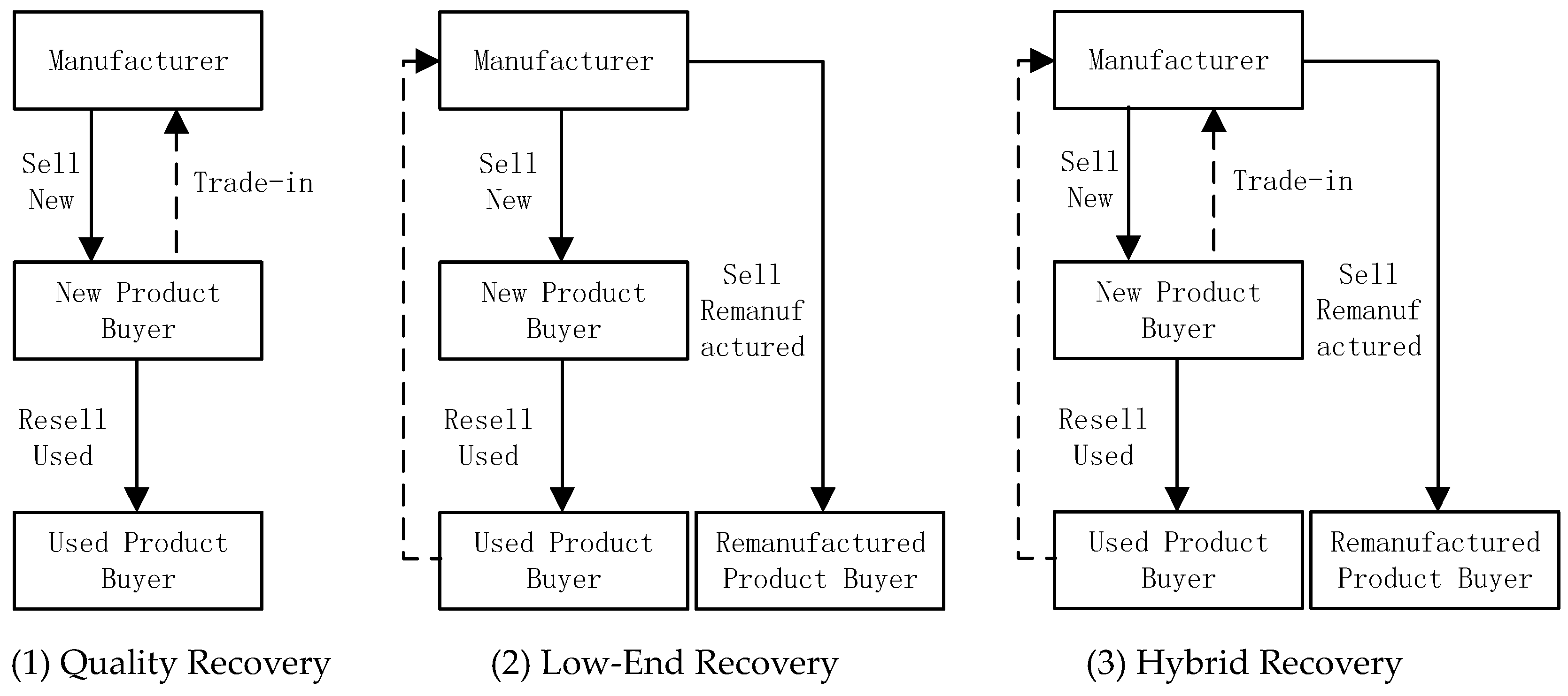
3.2. Recovery Strategy
The manufacturer’s decision for choosing a recovery strategy depends whether a used product or an end-of-life product is recovered and which type of product should appear in the secondary market. In what follows, we introduce the production, selling, and recovery flow for quality recovery, low-end recovery, and hybrid recovery, respectively. The details and process of each model are illustrated in Figure 1.
3.1.1. Quality Recovery
Under quality recovery, the manufacturer only sells new products to consumers and collects used products through trade-in. The components of used products are recovered into perfect condition and reused in the production process of new products. In this process, used products are first disassembled into components and then filtrated [40]. Useful components that are still in good condition can be reused in the production line or for after-sale service, after professional refurbishing and testing. This reduces the production and operational costs for the manufacturer. We denote the recovered value extracted from a used product as a fraction, of the production cost of a new product , where . If is high, the manufacturer can extract more value through the recovery and can make it cheaper to produce a new product. Note that using recovered components or new components to produce new products does not make any difference to user experience. Therefore, the manufacturer sells them at the same price, . We denote the demand for new products, used products, and the quantity of trade-in products as , , and , respectively.
This process is similar to quality recovery proposed by Atasu and Souza [3], where end-of-life products are recycled in a more sophisticated process, which can be considered as higher-end remanufacturing. The difference in our model is that we take the used product as the only source of quality recovery, rather than an end-of-life product. The reason is that used products are not used for too long a time from production, therefore, the components do not depreciate too much and are also easier and cheaper to recover to a new condition. However, end-of-life products often depreciate too much and are too costly to be recovered to new condition. This setting is closer to the way that manufacturers differentiate from the source for recovery.
3.1.2. Low-End Recovery
Under low-end recovery, the manufacturer sells both new and remanufactured products to consumers and collect end-of-life products for recovery. The process of low-end product recovery is to prolong the service life of end-of-life products and make them useful again. It can represent the mode of product repairing, refurbishing, and low-end remanufacturing, where recovered products are sold in the secondary market as lower quality substitutes for new products. The advantage of low-end recovery as a recovery strategy is that it provides end-of-life products with a relatively more profitable way to be recovered, rather than low efficiency material recycling. Hereafter, we simplify low-end recovery as remanufacturing.
We denote the cost of low-end recovery as . If the recovered value is high, more residual value can be extracted from the end-of-life product, which leads to a low value of . When end-of-life products are recovered, their service life can be extended for an extra period with the willingness to pay, , and can be resold in the secondary market at price . We denote the demand for new products, used products, and the quantity of remanufactured products as , , and , respectively.
3.1.3. Hybrid Recovery
Hybrid recovery refers to the combination of quality recovery and low-end recovery. Under this strategy, the manufacturer sells both new and remanufactured products to consumers and collects both used products and end-of-life products for recovery. On one hand, the manufacturer collects and recovers used products in the secondary market, which reduces the volume of used products in the secondary market. On the other hand, the manufacturer also recovers end-of-life products and puts them into the secondary market for reselling. Given this mixed strategy, the manufacturer can control the scale of the secondary market by either reducing or increasing the quantity of the product. Note that, although we assume that used products and remanufactured products are equally functional to consumers, the manufacturer cannot recover remanufactured products for the production of new products because remanufactured products are made up of low quality materials that are not qualified for quality recovery. We denote the demand for new products, used products, and the quantity of trade-in and remanufactured products as , , , and , respectively.
3.3. Environmental Impact and Recovery Standard
To analyze and compare environmental impact under each recovery strategy, we follow the idea from the LCA (life cycle analysis) framework [41,42,43]. In this paper, we consider that the total environmental impact of a single product happens in production, recovery, and disposal phases. The reason we do not consider the impact of the use phase is that we explicitly focus on the influence of the environmental impact caused by the recovery process. This helps us to focus on the role of the recovery standard and the environmental impact during the recovery process. Moreover, we can also limit our research to the products for which the environmental impact of the use phase is not significant compared to the production, recovery and disposal phases, such as electronic equipment and garments.
The total environmental impact of the manufacturer is calculated as the per-unit impact of products in each phase multiplied by the number of products in each phase. We denote as the per-unit production impact of a new product, which involves the materials and energy consumption during production. Then, we denote as the impact of the recovery process, which involves the additional material used to produce a recovered product, the impact of unused parts of products, and the energy consumption during the recovery process. At last, we denote as the per-unit disposal impact of an end-of-life product. The parameters referring to environmental impact are collected in a set of symbols, . In sum, the environmental impact under three product recovery strategies is given by the following:
Although it is profitable to reuse the old products, it is also costly to process the recovery as well as reducing the environmental impact of the unrecoverable part of old products. When recovering an old product, the most valuable parts, as well as the parts which are the easiest to recover, are recovered first, followed by the less profitable and less easy parts. It means that as the manufacturer increases the recovery portion of a product, the profit margin declines. As introduced in the research of Esenduran and Ziya [22] and Huang et al. [44], the manufacturer chooses the portion of recovery where the marginal recovery profit equals the margin processing cost. However, as the recovering technology is not high enough, the marginal recovery portion that guarantees the profitability of recovery is quite low. These manufacturers usually recycle only a small portion of the product and still leave a considerable portion for the landfill, which is still a threat to the environment.
In our study, policymakers set a mandatory recovery standard to restrict the lowest recovery portion to ensure the recovery is good enough for the environment, while the negative impact makes the recovery less profitable. We use to represent the mandatory recovery standard, which is the relative portion of environmental impact through product recovery, i.e., . We assume that quality recovery and low-end recovery obey the same recovery standard. In the analysis, we take as an exogenously given parameter and we assume that is always higher than the manufacturer’s profitable recovery margin, therefore they all follow the given recovery standard, , to optimize the profit. Moreover, given this condition, we also assume that the enhancement of recovery technology only increases the recovered value, but does not decrease the recovery standard. In the analysis, we assume that a tradeoff exists between the recovered value and recovery impact, therefore, a more stringent recovery leads to lower recovered values. While we do not specifically model this tradeoff, it is considered it in the analysis. In sum, we use the recovered values ( and ) and the recovery standard () to reflect the performance of the manufacture’s recovery.
3.4. Specification of the Game
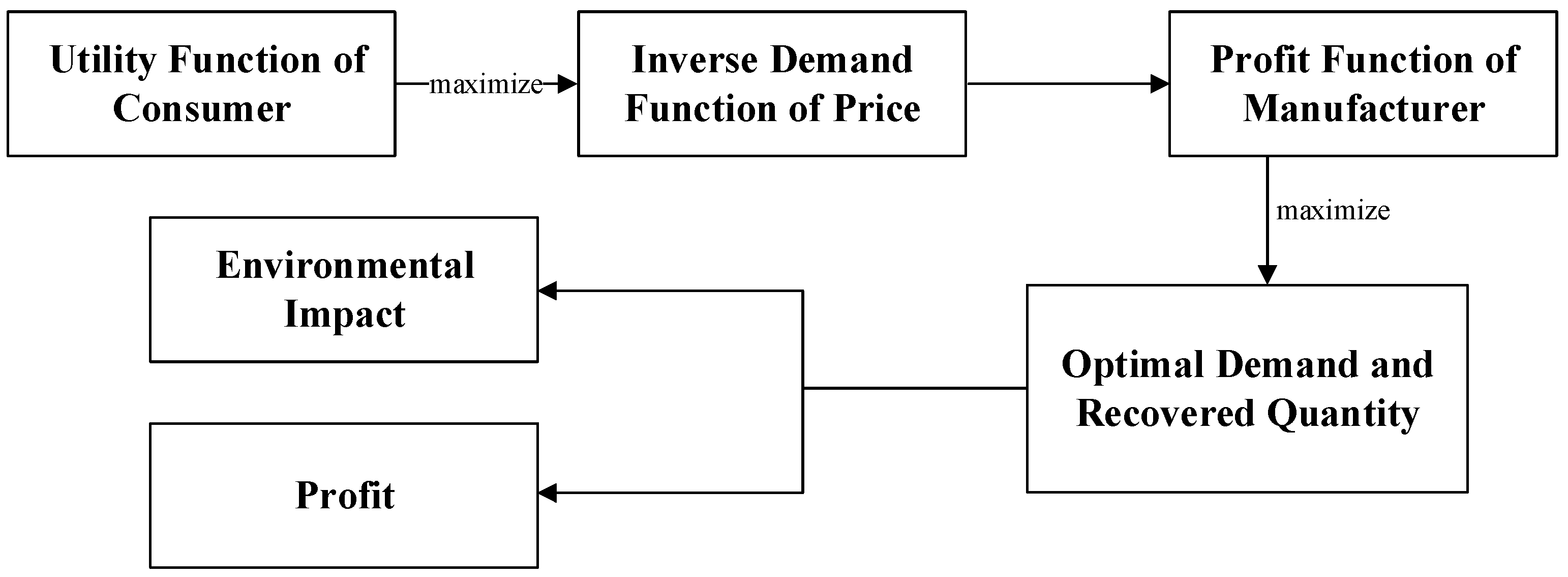
We develop a sequential game where the manufacturer and consumer make their decisions sequentially. Specifically, in each period of the dynamic game, the manufacturer first determines the quantity of new product production and the quantity of recovered product, and these decisions reveal the price of each type of product under the market clearing condition. Then, consumers decide whether to buy and which product to buy based on the price of the product and their willingness-to-pay. The solving process follows backward induction and the details are shown in Figure 2. We first solve the inverse demand function of the price according to consumers’ utility function, then we substitute the result into manufacturer’s profit maximizing problem. After solving the manufacturer’s problem, we substitute the results of the demand and recovery quantities into the function of profit and the environmental impact function and obtain the results.
The manufacturer and consumer make their decision by maximizing their net utility or profit with a discount factor, . We also assume that the manufacturer has an unlimited production capacity to satisfy all demand in the market. Based on the sequential feature of the game, we solve for the consumer’s subgame perfect equilibria using backward induction before analyzing the manufacturer’s equilibrium strategy.
3.5. Consumer Demand under Different Recovery Modes
In this section, we solve the consumer’s subgame perfect equilibria strategy and obtain an inverse demand function under different recovery strategies.
3.5.1. Quality Recovery
Given our setting of quality recovery, there are four undominated two-period actions for the consumer in period . Let denote the action vector for consumers under quality recovery, where , , , and represent buying new products, buying trade-in products, buying used products, and not using any product, respectively. According to the analysis in Appendix A.1, we can know that, at most, 4 undominated and time-independent two-period strategies exist, i.e., purchasing new products through trade-in (), purchasing new products and reselling used products inherited from last period (), purchasing used products (), and inactive ().
As used products are all inherited from new products from the former period, the quantity of new product in the current period should equal the sum of trade-in products and resold used products, i.e., . Moreover, as consumers can always choose to resell their used products at price , the only situation in which trade-in is attractive to consumers is the low trade-in price. Thus, we assume that the trade-in price can always compensate for the loss of not reselling, i.e., , and the manufacturer will always choose to optimize the profit. Given the condition of the market clearing price, with respect to the scale of the secondary market, , and through the calculation process in Appendix A.1, we can obtain inverse demand functions and .
3.5.2. Low-End Recovery
Next we investigate consumers’ actions under low-end recovery, where the manufacturer does not recover used products collected by trade-in, but recovers end-of-life products into remanufactured products and sells them in the secondary market. Let denote the 4 single period actions under this strategy, where represents buying remanufactured product and the other actions stay the same as with quality recovery. According to the analysis in Appendix A.2, we can know that there exists, at most, 4 undominated time-independent two-period strategies, i.e., purchasing new product and reselling used product inherited from last period (), purchasing used product (), purchasing remanufactured product (), and inactive ().
As the scale of the secondary market contains all used products and remanufactured products, the scale of the secondary market is noted as , where . Given the condition of market clearing price with respect to the scale of the secondary market , and through the calculation process in Appendix A.2, we can obtain inverse demand functions and .
3.5.3. Hybrid Recovery
Next, we investigate consumers’ actions in the end-of-life product recovery model, where the manufacturer recovers both used products and end-of-life products and both used products and remanufactured products are sold in the secondary market. Let denote the action vector for consumers in hybrid recovery, which includes all possible actions in quality and low-end recovery. According to the analysis in Appendix A.3, we can know that there exists, at most, 5 undominated and time-independent two-period strategies, i.e., purchasing new products through trade-in (), purchasing new products and resell used products inherited from last period (), purchasing used products (), purchasing remanufactured products (), and inactive ().
Several quantity relationships are satisfied because of the integration of two types of recovery. First, the quantity of trade-in products and resold products equals the quantity of new products, i.e., . Second, the scale of the secondary market is the sum of the resold products and the remanufactured products, which is equivalent to . Third, the price of trade-in products satisfies . Given the condition of the market clearing price, with respect to the scale of the secondary market , and through the calculation process in Appendix A.3, we can obtain the inverse demand functions and .
4. Pure Recovery Strategies
In this section, we examine the firm’s optimal production quantity of new products, the optimal quantity of recovery, and the corresponding environmental impact under quality recovery and low-end recovery (remanufacturing). We also compare the profit and environmental impacts of these two recovery strategies.
4.1. Quality Recovery
Under quality recovery, used products are collected through the trade-in program and there are only used products in the secondary market if they are not totally recovered. In each period, the manufacturer jointly decides the product quantity of new products, , and the recovered quantity of used products, . Therefore, the quantity of resold used products in the secondary market is given by . The profit-maximizing problem which is jointly concave in and is given by the following:
The first two constraints guarantee the non-negative quantity of trade-in products and new products. Meanwhile, the quantity of trade-in products is not more than new products in each period. The third constraint ensures that there is no difference in net utility for consumers to trade-in or to resell used products. The following proposition summarizes the manufacturer’s optimal decision under quality recovery.
Proposition 1.
Under quality recovery, there exist thresholds,, where, such that
- (1)
- If, the manufacturer does not recover the used products, all used products are resold in the secondary market.
- (2)
- If, the manufacturer trades-in and recovers part of the used products and the other used products are resold in the secondary market.
- (3)
- If, the manufacturer trades-in and recovers all used products in the market and the secondary market does not exist.
The proof of Proposition 1 is given in Appendix A.4.
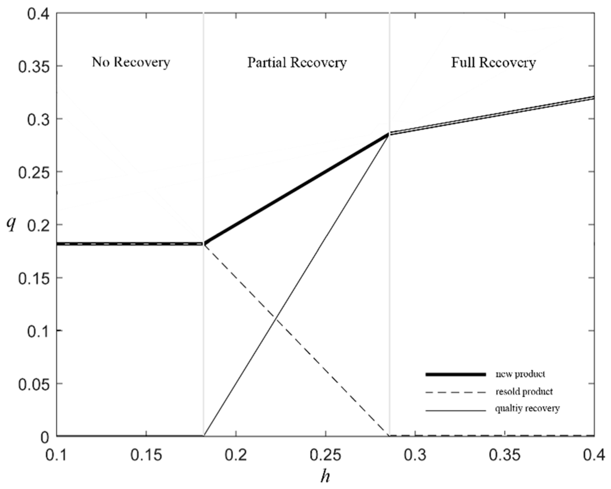
The main result in Proposition 1 shows that the manufacturer’s optimal decision recovery quantity is mainly driven by the recovered value. For the low recovered value (), the manufacturer would not collect any products for recovery, which leads to a pure reselling strategy, since the profit of recovery is not enough to compensate for the cost of product collection in the trade-in program. When the recovered value increases to a medium level (), the manufacturer would collect and recover part of the used products in the secondary market. The reason is that the higher recovered value makes it profitable for manufacturers to recover the used products. However, when the manufacturer buys back more used products, the used products in the secondary market become scarce and the price of used products increases. This leads to a decline of marginal profit for recovery and the manufacturer does not increase the recovery quantity when the marginal profit equals the collection cost. When the recovered value is high (), the manufacturer would collect all used products in the secondary market, because the recovery is profitable enough to allow the manufacturer to buy back all used products and rule out the entire secondary market. This is the most ideal situation for recovery economics. Figure 3 clearly reveals that, as the recovered value turns from low to high, the quantity of new and recovered products increases weakly and the quantity of resold products decreases weakly.
The results of Proposition 1 also show that the durability of the product also affects the choice of recovery strategy. When , the threshold is . This indicates that the manufacturer recovers used products even if the recovered value is 0. This is because, when the durability of the product is low the price of used products is also low, and this lowers the cost for collection. Therefore, the manufacturer would like to spontaneously remove used products from the secondary market to alleviate the cannibalization effect.
4.2. Low-End Recovery
Under low-end recovery, used products are all resold in the secondary market. The end-of-life products can be recovered and be functional again as remanufactured products. This is equivalent to prolonging the lifespan of used products. In each period, the manufacturer jointly decides the production quantity of the new products, , and the remanufacturing quantity of used products . Therefore, the total quantity of used products in the secondary market is given by . The profit-maximizing problem, which is jointly concave in and is given by the following:
These constraints ensure the non-negative of production quantity of new products and remanufacturing quantity. Meanwhile, the quantity of remanufactured product is not more than new or used products in each period. The following proposition summarizes the manufacturer’s optimal decision under low-end recovery:
Proposition 2.
Under low-end recovery, there exist the thresholds,, where, such that
- (1)
- If, the manufacturer does not recover end-of-life products;
- (2)
- If, the manufacturer recovers part of end-of-life products;
- (3)
- If, the manufacturer recovers all end-of-life products.
The proof of Proposition 2 is given in Appendix A.5.
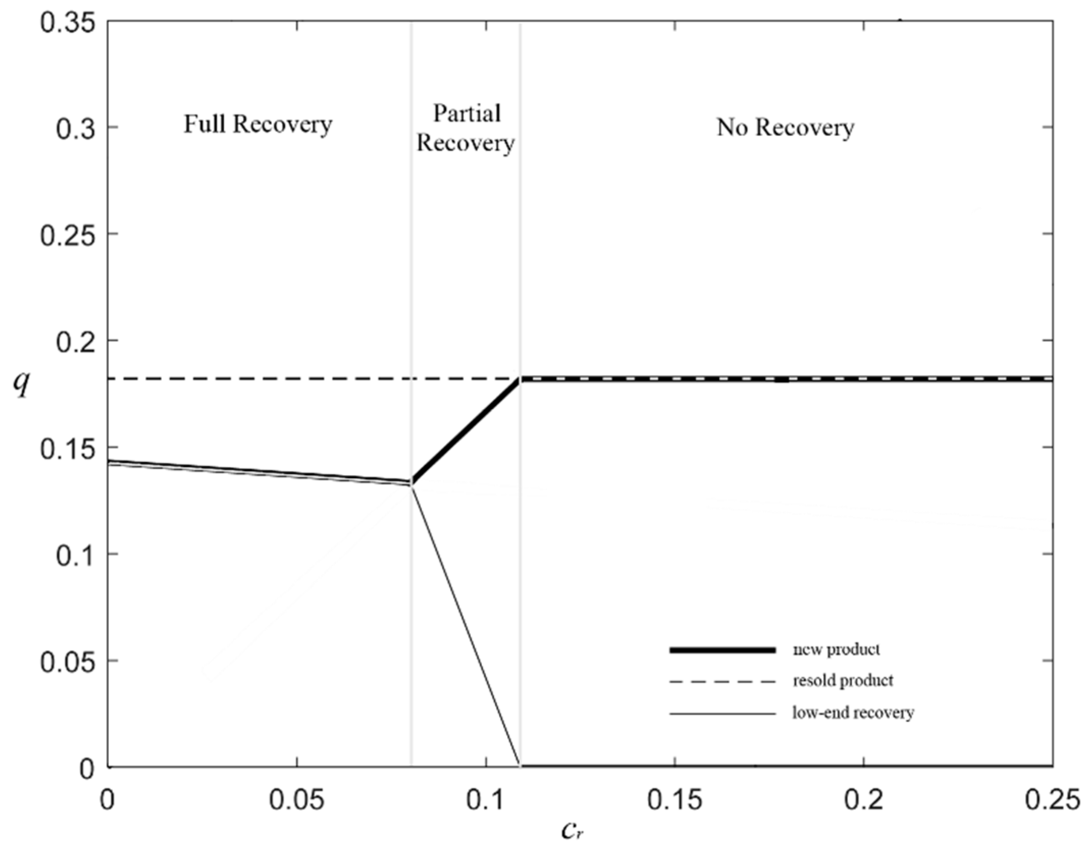
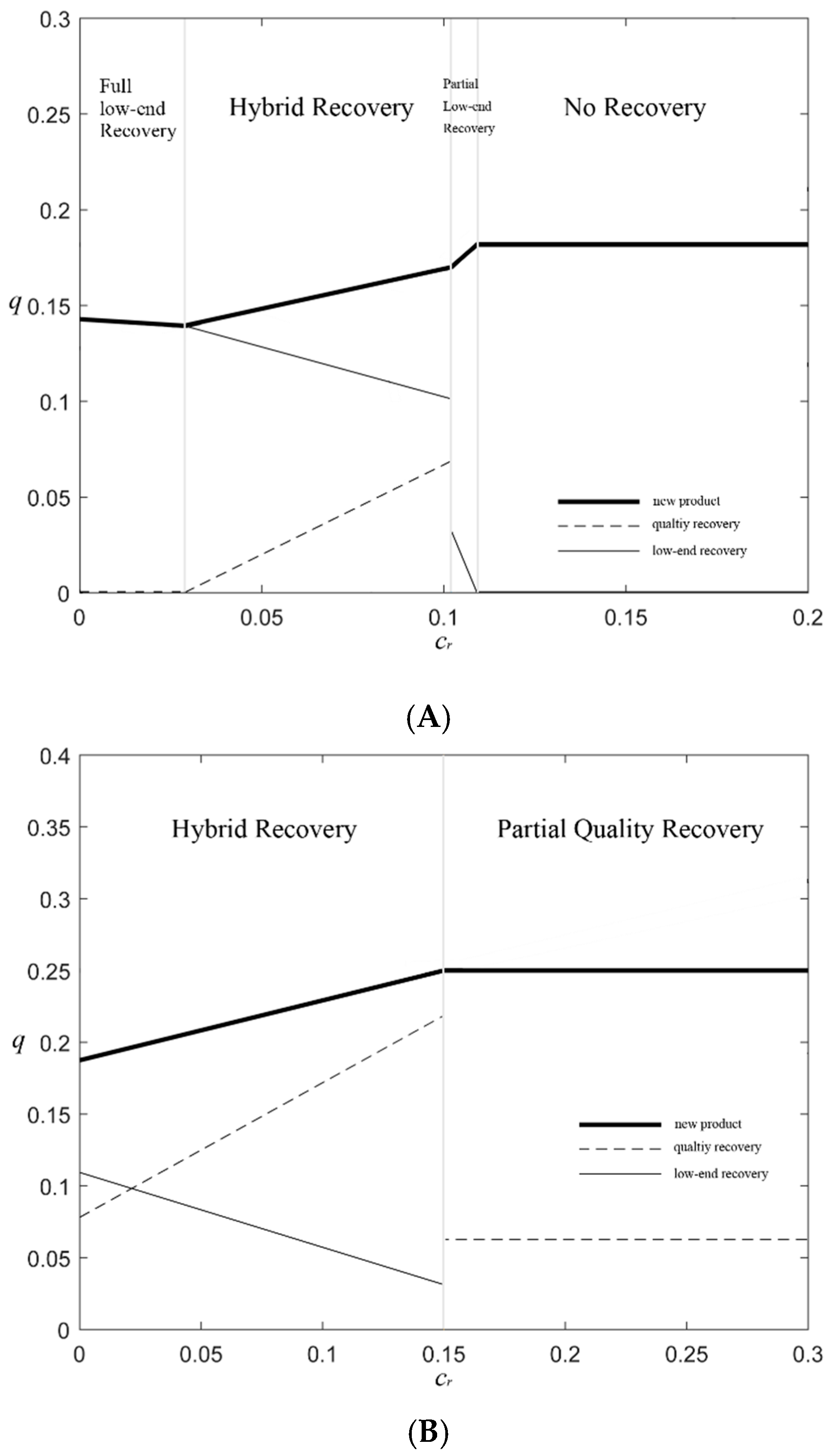
Proposition 2 reveals that whether low-end recovery is more profitable than pure reselling primarily depends on the recovered value of remanufacturing. When the remanufacturing cost is high (), it represents a low recovered value, therefore the recovery is not profitable enough and the manufacturer would rather adopt the pure reselling strategy. With the increase of the recovered value, the remanufacturing cost decreases to a medium range (), making the recovery profitable. While, with the increase of recovered quantity, the scale of the secondary market expands. This decreases the price of both used and remanufactured products and the profit margin for the recovery declines. When the quantity of remanufactured products is large enough, the profit margin for recovery becomes 0 and the manufacturer will not recover more end-of-life products. When the recovered value is extremely high, the remanufacturing cost would become low enough () to allow all end-of-life products to be recovered. Figure 4 clearly shows that as the recovered value turns from low to high, i.e., the remanufacturing cost turns from high to low, the quantity of new product first decreases weakly and then increases, the quantity of recovered, and resold product increases weakly, the quantity of resold products keeps unchanged.
Moreover, consumers’ valuation of used and remanufactured products also affects the choice of low-end recovery. When the valuation of remanufactured product is low (), it leads to . Therefore, no matter how profitable the recovery is, it is not optimal for the manufacturer to recover any end-of-life product. Additionally, when the valuation becomes higher (), it leads to and , thus partial recovery starts to be potentially profitable. When , full recovery starts to be potentially profitable. This result implies that if consumers value used and remanufactured products more, low-end recovery is more appealing to the manufacturer.
4.3. Environmental Impact
As the manufacturer’s target is profit maximizing, the decision of the recovery strategy does not depend on the environmental impact, making the environmental impact an endogenously determined result. Next, we analyze how the recovered value impacts the environmental impact under both recovery strategies and how the mandatory recovery standard, , should be set to ensure that the recovery is environmentally superior to pure reselling as well, as achieving sustainable environmental improvement.
Proposition 3.
There exist thresholds,,,, such that
- (1)
- When the manufacturer partially recovers used products, if, the environmental impact decreases inand the environmental impact is lower than pure reselling.
- (2)
- When the manufacturer recovers all used products, the environmental impact always increases inand the environmental impact is lower than pure reselling only if, where.
- (3)
- When the manufacturer partially recovers end-of-life products, if, the environmental impact decreases asdecreases and the environmental impact is lower than reselling.
- (4)
- When the manufacturer recovers whole end-of-life products, the environmental impact always increases asdecreases. The environmental impact is lower than pure reselling only if, where.
The proof of Proposition 3 is given in Appendix A.6.
Proposition 3 provides the comparison of environmental impact between pure reselling and the two pure recovery strategies. The result shows that, for both types of recovery strategies, partial recovery is greener than pure reselling only if the recovery impact is lower than a certain threshold, which means the environmental impact of recovering old versions of products should be lower than the overall impact of producing a new product and disposing an end-of-life product. The reason is that although product recovery can reduce new material for building new products, it also leads to more demand for new products. Meanwhile, if the unrecovered part of the product is huge, it is possible that the environmental impact caused by increased recovered quantity can backfire and deteriorate the environment. Additionally, when the manufacturer changes from partial recovery to full recovery, the recovery standard that guarantees the recovery being environmentally superior becomes more stringent.
Proposition 3 also shows that when the manufacturer increases the recovered value due to the enhancement of recovery technology, the environmental impact can be improved if the manufacturer still adopts partial recovery strategy. However, when the recovered value is improved to a level where full recovery is optimal, the continuous enhancement of recovery technology may deteriorate the environment.
This result provides insight to the policymaker. For the purpose of continual enhancement of environmental performance, the government should prevent manufacturers from adopting the full recovery strategy and regulate them for keeping partial recovery. To this end, lowering the recovery standard is a potential solution, because setting a more stringent recovery standard can lower the total recovered value and force manufacturers to stay in the range of the recovered value where partial recovery is optimal. It is also a way to progressively transfer the manufacturer’s profit-driven motivation and technology enhancement into an environmental improvement. Thus, in the following discussion, we assume that the policymaker would not allow firms to adopt full recovery by setting regulations and full recovery is ruled out from the analysis.
4.4. Win-Win Condition
As introduced in former sections, two recovery strategies are both applicable in improving environmental performance. Moreover, it is more interesting to discuss when the firm’s profit-maximizing choice of recovery strategy is environmentally superior as well. The next proposition discusses this question.
Proposition 4.
Considering a partial recovery strategy for both used products and end-of-life products
- (1)
- There exist, such that when, quality recovery is more profitable than low-end recovery;
- (2)
- When, quality recovery is strictly greener than low-end recovery. When, there is, such that when, quality recovery is greener, otherwise, low-end recovery is greener;
- (3)
- ,decreases in.
The proof of Proposition 4 is given in Appendix A.7.
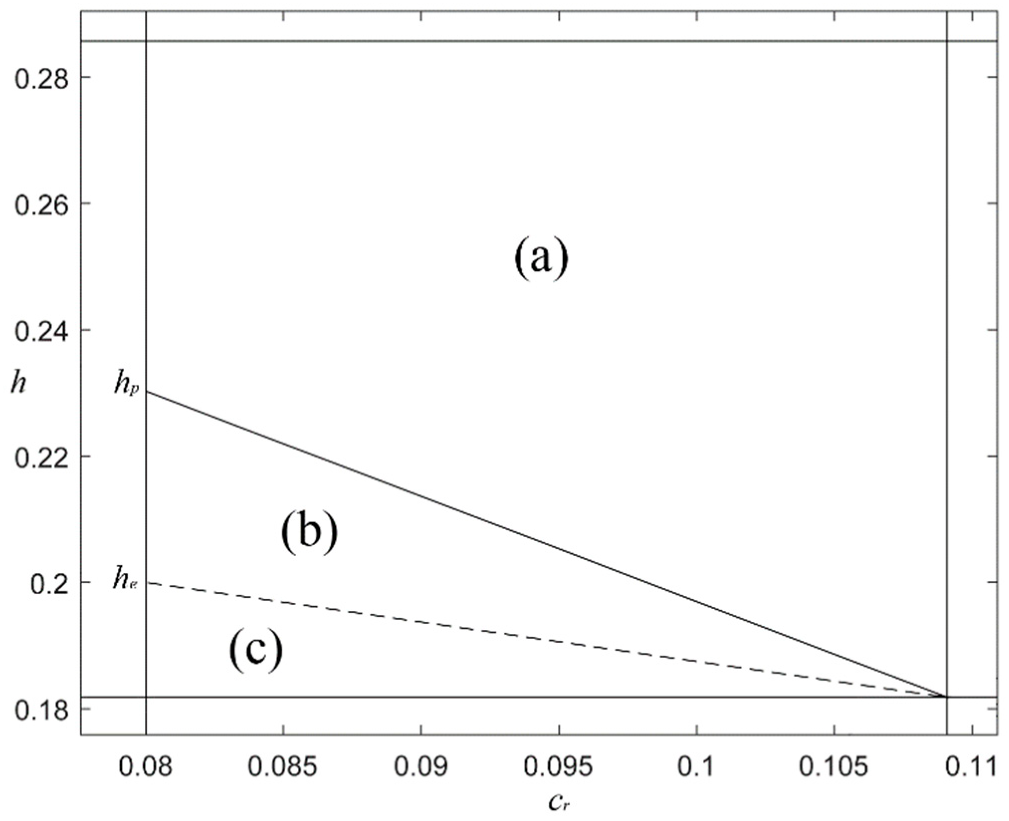
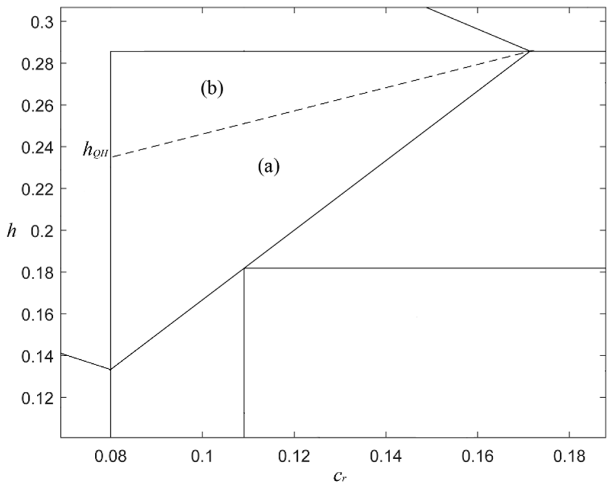
The result in Proposition 4 reveals that there are several cases wherein the manufacturer can obtain a win-win outcome under partial recovery. When the recovery standard is not too low (), partial quality recovery is a win-win strategy only if the recovered value from quality recovery is relatively high . At this time, quality recovery is always greener than pure reselling and low-end recovery is always environmentally inferior to pure reselling. Therefore, as long as quality recovery is more profitable, it is also a win-win recovery strategy. When the recovery standard is high (), used products’ partial recovery is a win-win strategy only if the recovered quality of recovery is high enough (, (a) in Figure 5). End-of-life products’ partial recovery is a win-win strategy only if the recovered value of quality recovery is low enough (, (c) in Figure 5). The reason is that, at this time, both of the recovery strategies can get environmental improvement by increasing the recovered value. When the recovered value from the used products is low, it is possible for remanufacturing to be greener than quality recovery, especially when the remanufacturing cost is low. Interestingly, when the recovered value of the used product is in the medium range (, (b) in Figure 5), the manufacturer will never achieve the win-win outcome. As illustrated in Figure 5, at this time, the recovered value of used manufacturers is not enough to make quality recovery more profitable than low-end recovery, while it is already high enough to make quality recovery environmentally superior than low-end recovery.
Comparing these two recovery strategies, quality recovery may have a higher potential for both profit and environmental improvement, because it is always greener when it is more profitable as well. The result also shows us that, under the pure recovery model, the profit-maximizing target can drive firms to choose environmentally inferior decisions, especially when it’s greener to adopt quality recovery but not profitable enough to change from low-end recovery to quality recovery.
5. Hybrid Recovery Strategy
In this section, we discuss the feasibility and feature of the hybrid recovery strategy. We assume that the manufacturer can choose quality recovery and low-end recovery at the same time, where the manufacturer can adjust the scale of the secondary market, not only by removing used products from the secondary market, but also putting remanufactured products in the secondary market. Thus, the quantity of total products in the secondary market is given by . The profit-maximizing problem, which is jointly concave in , , , is given by the following:
The first constraint guarantee is that the sum of recovered used products and recovered end-of-life products is less than the production quantity of new products. The following two constraints guarantee the non-negativity of both recovered quantities. The last constraint ensures that there is no difference in net utility for consumers to trade-in or to resell used products.
5.1. Profitability
Proposition 5.
There exist thresholds,,, such that when,,are all satisfied, it is optimal for the manufacturer to adopt the hybrid recovery strategy.
The proof of Proposition 5 is given in Appendix A.8.
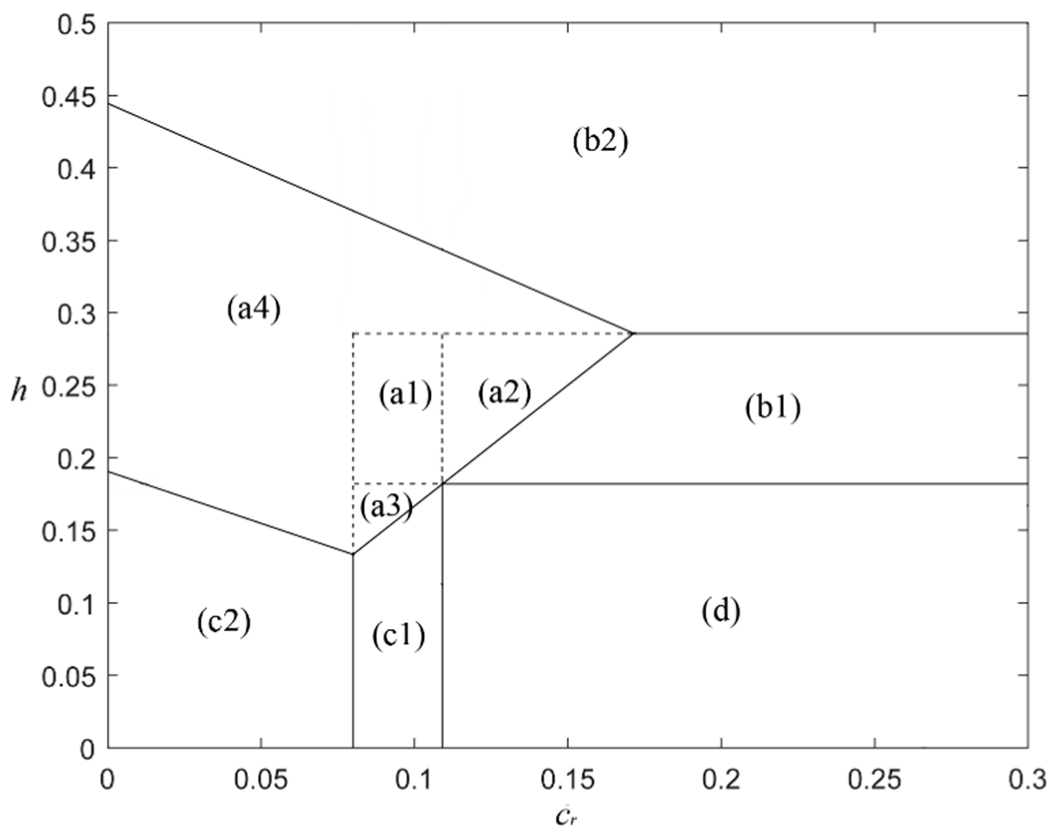
As shown in Proposition 5 and illustrated in Figure 6, the optimality of hybrid strategy depends on the relationship between and . If and are both within the optimal range for the manufacturer to adopt a partial recovery strategy ((a1) in Figure 6), the manufacturer will always prefer hybrid recovery strategy. Moreover, even when one type of recovery is less profitable on its own, it may still be adopted in the hybrid recovery strategy only if the other type of recovery is profitable ((a2) and (a3) in Figure 6). This raises the suspicion that the profitability of either type of recovery enhances the profitability of the other recovery strategy, which forms a synergistic effect between the two recovery strategies. The result also shows that when and are within the range where it is optimal for the manufacturer to adopt the full recovery strategy ((a4) in Figure 6), the hybrid recovery strategy can be optimal, while we exclude this situation hereafter.
An interesting phenomenon is that the hybrid recovery when can be seen as another type of full recovery strategy because, as we can see in the proof of Proposition 5, the only scenario where both types of recovery coexist is where the manufacturer’s products are all recovered and part of them follow quality recovery and the others follow low-end recovery. At this time, although the manufacturer is not able to recover all products under the pure recovery strategy, it can achieve full recovery, which simulates the recovery activities even with a low recovered value.
The synergy effect is more clearly reflected in the price of used and remanufactured products. According to the proof of Proposition 5, , we can easily know that, and increase in both and . This implies that, as the recovered value of quality recovery increases, the manufacturer trades-in more recovered product and lowers the quantity of used products in the secondary market. This further increases the price of used products and remanufactured products, such that a higher recovered value of quality recovery leads to higher profits for selling remanufactured products. In the same sense, when the recovered value of low-end recovery increases, decreases correspondingly and the manufacturer would recover more end-of-life products and expand the scale of the secondary market. This further decreases the price of the used products and trade-in prices and increases the profitability for quality recovery. Under this case, as the two types of recovery models share the total demand of quantity, the synergy effect is not shown in the recovered quantity, while it is clearly shown in the price of used and remanufactured products.
Aside from the synergy effect, a contradiction effect also exists. According to the proof of Proposition 5, , , it is clear that decreases in and increases in , so the increase of the recovered value of quality recovery can negatively influence the recovery quantity of low-end recovery and the increase of the recovered value of low-end recovery can negatively influence the recovery quantity of quality recovery.
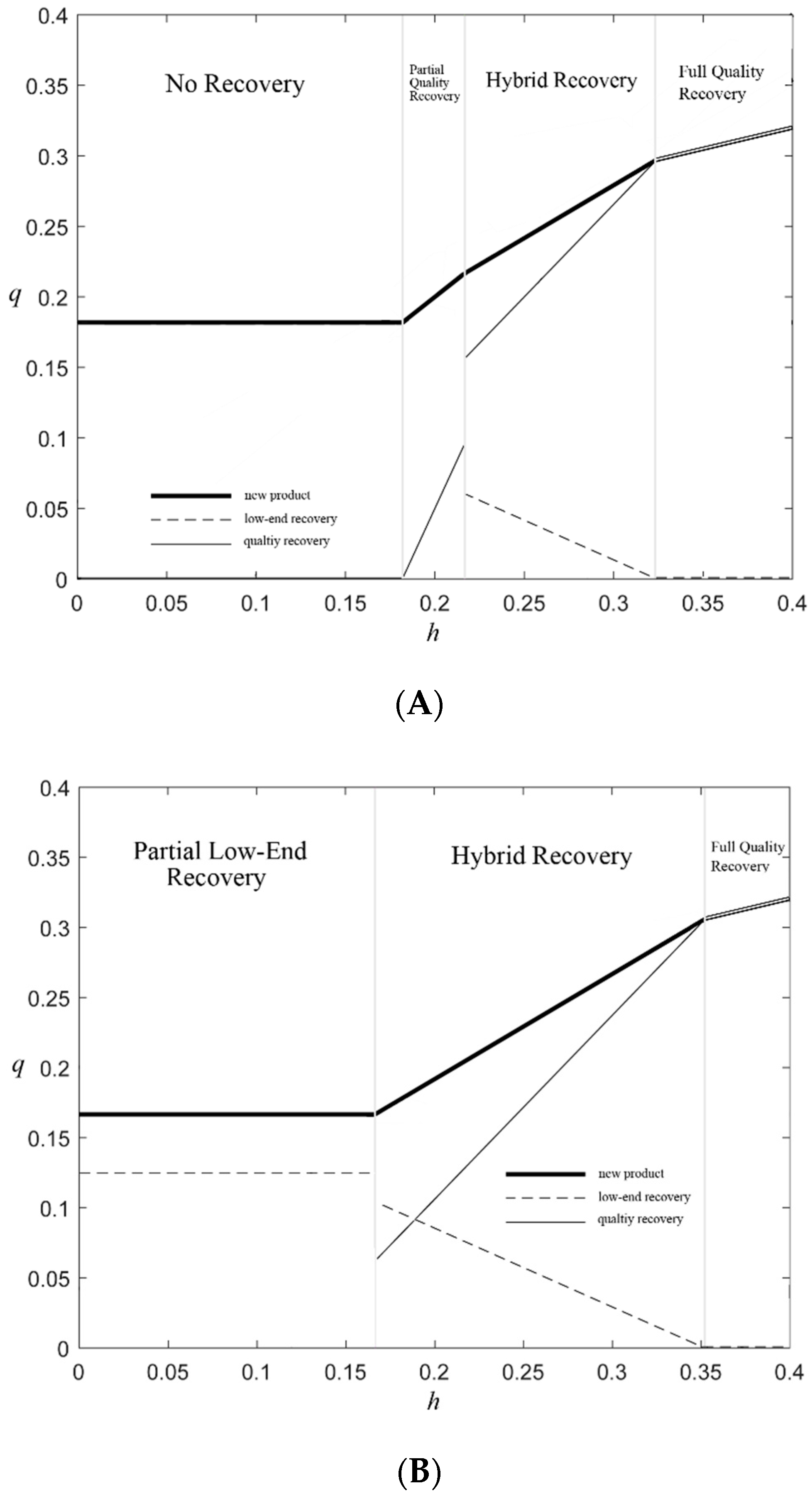
These two effects are clearly shown in Figure 7 and Figure 8. In Figure 7, when surpasses the lower threshold to adopt hybrid recovery, there is a jumping point for the quality recovery quantity by introducing low-end recovery. At the same time, originally is not low enough for firms to implement low-end recovery. However, by adopting hybrid recovery, low-end recovery can be profitable. The contradiction relationship can be also seen in Figure 7, because in hybrid recovery, the increase of one type of recovery always declines the other type of recovery. Figure 8 shows the same situation from the perspective of low-end recovery.
5.2. Environmental Impact
Next, we discuss the environmental impact of hybrid recovery. We consider the situation where the manufacturer changes from adopting a pure recovery strategy to a hybrid recovery strategy, such that the maximum recovery standard should be satisfied, i.e., for low-end recovery and for quality recovery.
Proposition 6.
(1) When, quality recovery is always greener than hybrid recovery. When, there exists, if, hybrid recovery is greener than quality recovery.decreases in.
(2) When, hybrid recovery is always greener than low-end recovery.
The proof of Proposition 6 is given in Appendix A.9.
Proposition 6 shows that hybrid recovery is a perfect substitute for low-end recovery. Meanwhile, hybrid recovery can not only improve the environmental impact of quality recovery, but can also deteriorate it as well.
For low-end recovery, when low-end recovery is greener than pure reselling (), low-end recovery is completely ruled out by hybrid recovery, as it is more profitable and environmentally superior at the same time. For quality recovery, when the recovery standard is not high (), hybrid recovery deteriorates the environmental impact. When the recovery standard is high (), hybrid recovery improves the environmental performance for quality recovery when the recovered value is relatively low (), but deteriorates the environment when the recovered value is relatively high ().
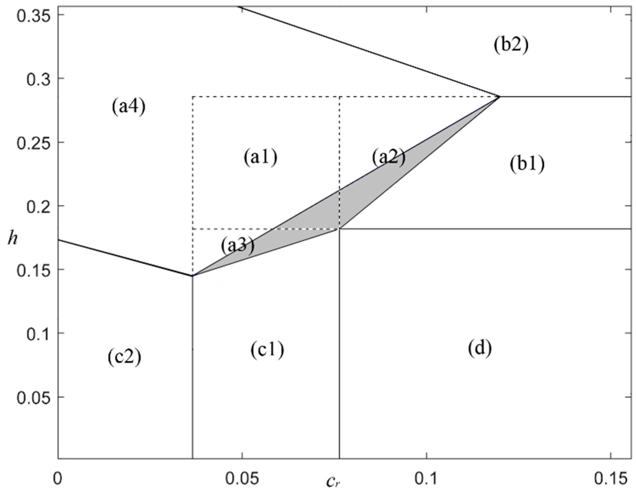
The condition where the positive and negative influence on win-win improvement happens is more clearly illustrated in Figure 9. By implementing hybrid recovery, low-end recovery is able to achieve win-win improvement by introducing extra quality recovery (region (c) and (d) in Figure 9). Especially, a decision area that cannot get a win-win situation in Proposition 4 can be improved by hybrid recovery (region (b) in Figure 5). The win-win improvement also happens to quality recovery with a low recovered value by introducing extra low-end recovery when the recovered standard is high (region (a) in Figure 9). However, when the recovered value of quality recovery is high (region (b) in Figure 9), hybrid recovery should be forbidden or negatively interfered by the policymaker. In this situation, enhancing the recovery standard or incentive firms to adopt pure quality recovery helps hybrid recovery to get better environmental performance, especially when firms are not very good at quality recovery. As the technology of quality recovery becomes high enough, it would eventually be the most ideal recovery strategy. Before this happens, hybrid recovery would be an intermediate strategy to get a higher price and environmental performance.
5.3. Impact of the Recovery Standard
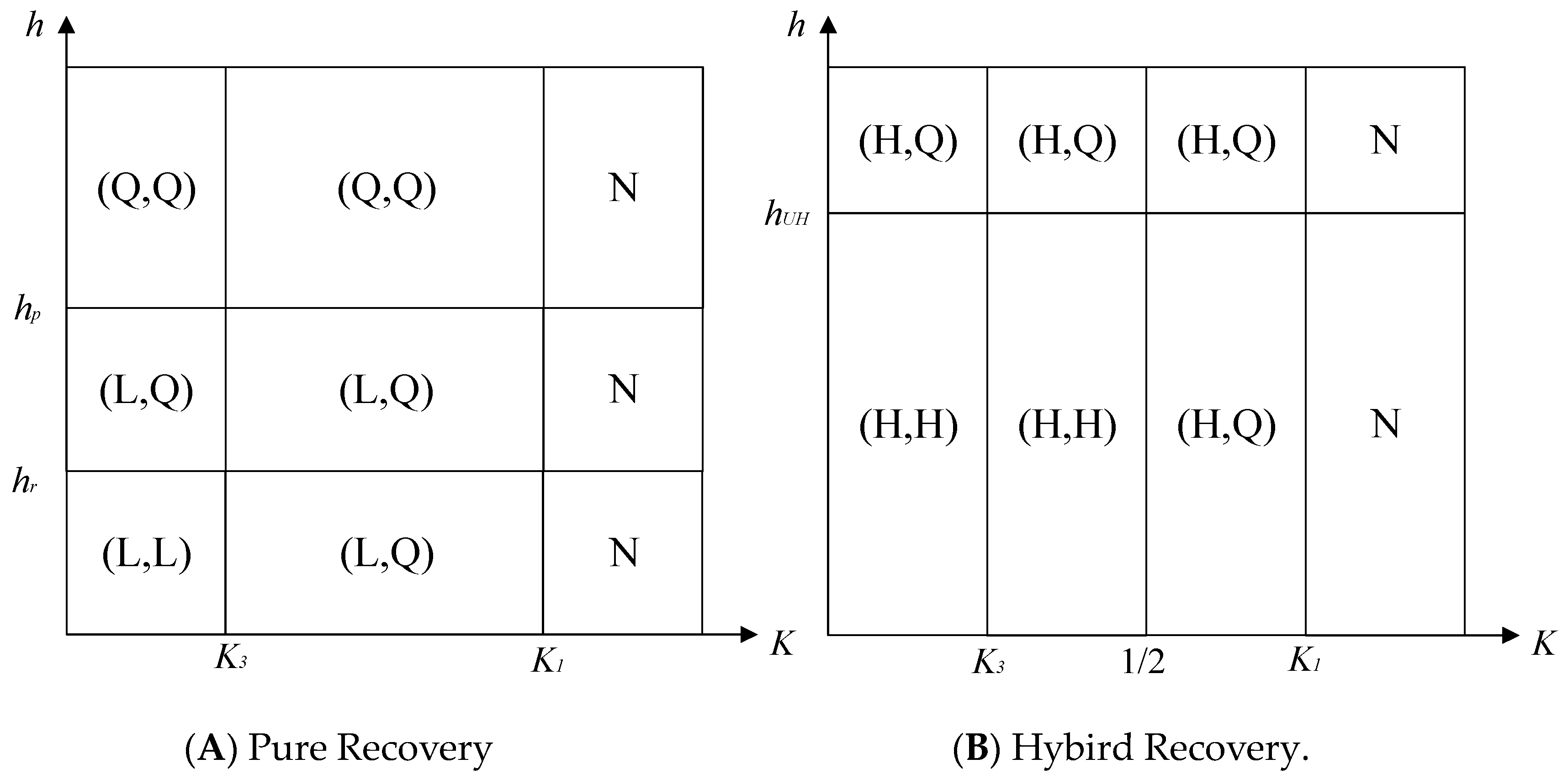
At last, we summarize the impact of the recovery standard in determining the win-win condition and the technologically sustainable condition. The results in former propositions are concluded in Figure 10. We can see that the recovery standard greatly influences the optimality of each strategy. Specifically, when the recovery standard is not too stringent, quality recovery is always environmentally superior, when recovery standard is stringent, low-end recovery and hybrid recovery can be environmentally superior to quality recovery. As a stringent recovery standard can also decrease the value of , policymakers can always implement a stringent recovery standard to keep the manufacture in the (L,L) or (H,H) regions. It is also obvious in Figure 10 that hybrid recovery expands the win-win region when is low, making it easier and more profitable to obtain a win-win condition because of the less stringent recovery standard.
5.4. Impact of Recovery Technology
As stated in Proposition 3, we can conclude that, under pure recovery, as long as the recovery standard is stringent enough, the development of recovery technology can always benefit the environment. In this section, we discuss the recovery technology under hybrid recovery.
Proposition 7.
Under the hybrid recovery model, the environmental impact decreases in bothand.
The proof of Proposition 7 is given in Appendix A.10.
Proposition 7 shows us the impact of the recovered value on the environmental impact under the hybrid recovery strategy. We find that as the recovered value of quality recovery increases, environmental impact is lowered, therefore the development of the manufacturer’s recovery technology benefits the environment. However, the increase of the recovery value of end-of-life products leads to higher environmental impact, which means the development of the manufacturer’s recovery technology of low-end recovery will cause more damage to the environment. Thus, the hybrid strategy is an ideal strategy for the continual development of quality recovery technology, but not for low-end recovery technology.
Given this condition, policymaker may consider implementing different recovery standards with respect to these two recovery strategies. In particular, policymakers should set a more stringent recovery standard for low-end recovery to resist the portion of low-end recovery in hybrid recovery. However, a too stringent recovery standard also does not work well, because it makes too high and the manufacturer may turn to pure quality recovery and may deteriorate the environment when . Under this situation, policymakers should keep the minimum quantity of low-end recovery to guarantee the optimality of hybrid recovery.
6. Extension
In this study, we have discussed the situation where consumers have the same willingness-to-pay for used products and remanufactured products. In this section, we relax this assumption and examine whether our main results still hold if consumers value used products and remanufactured products differently. As we defined before, consumers show a willingness-to-pay, , for used products and willingness-to-pay, , for the remanufactured products. We define to characterize the relationship between and , where . Therefore when , the remanufactured product provides lower value to the consumer and when , the remanufactured product provides higher value to the consumer.
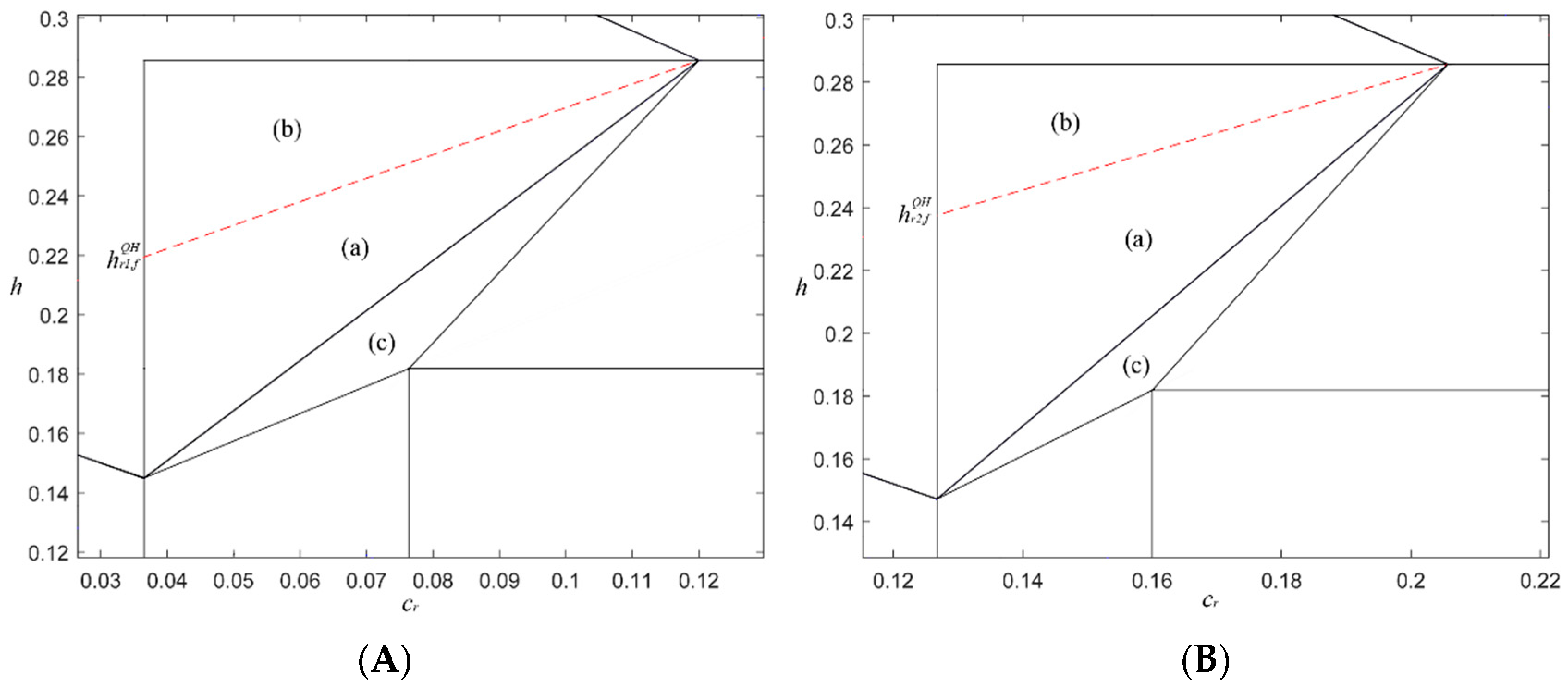
First, we examine the win-win outcome under the pure recovery strategy. Recall the results we obtained in the proofs of Proposition 1 and Proposition 2. We can know the profit and environmental impact in different ranges of under pure and partial recovery strategies, as well as the boundary of which determines the optimality of each recovery strategy (See Appendix A.10). As we can see, the result shown in Figure 11 is similar to Figure 5. Specifically, (a) and (c) represents the win-win condition for pure quality recovery and low-end recovery, respectively, and (b) represents the condition where the win-win outcome is achieved. This result implies that the value of does not affect our structure results in Proposition 4.
Second, we check the optimal decision of manufacture considering different values of . According to the result in Proposition 5, we can obtain a similar structural result of the manufacturer’s with As we can see in Figure 12, there are also 3 regions in which hybrid recovery is optimal ((a1), (a2), (a3)). The only difference is that a decision area exists where the manufacturer does not recover all products under hybrid recovery (shaded region in Figure 12). Moreover, the synergy effect is also clearly shown ((a2) and (a3) in Figure 12). This does not affect our structure result in Proposition 5.
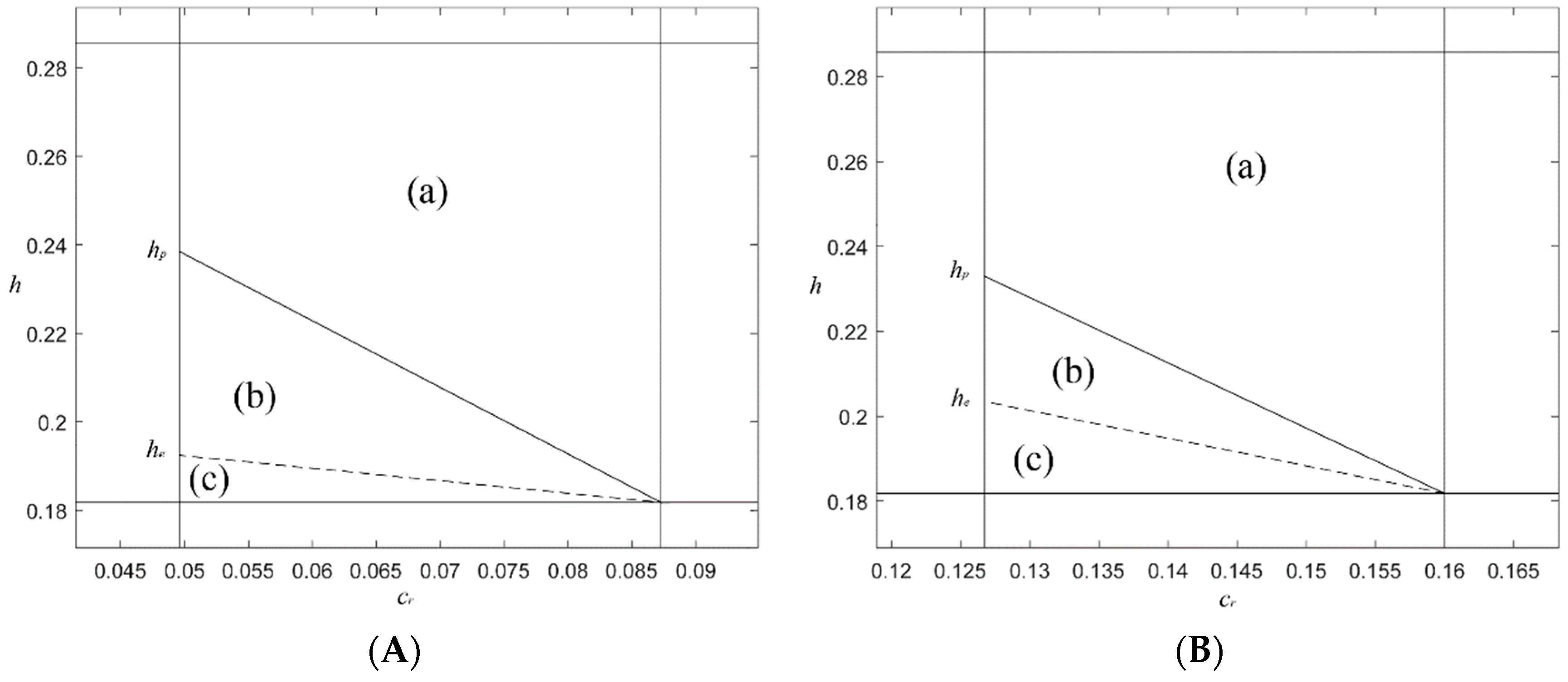
Finally, we investigate the win-win condition considering hybrid recovery. Recall the results we obtained in the proof of Proposition 5. We can know the profit and environmental impact within different ranges of under pure and partial recovery strategies. We can also obtain the theoretical boundaries of , which determine the optimality of each recovery strategy. By numerically examining these boundaries under different settings of , , and , we test our structure result in Proposition 6. All details are given in Appendix A.10. Specifically, the theoretical boundaries that determine the optimality between low-recovery and hybrid recovery do not fall on the parameter range where hybrid recovery is optimal. This means that the conclusion that hybrid recovery is greener than low-end recovery is robust. Moreover, the theoretical boundaries that determine the optimality between partial hybrid recovery and quality recovery do not fall on the available parameter range either. The boundary always falls on the parameter range of full hybrid recovery. This means that partial hybrid recovery is always environmentally inferior to quality recovery. Additionally, as we can see in Figure 13, involving different values of does change our structure result such that hybrid recovery is greener than quality recovery when is low ((a) in Figure 13) and is environmentally inferior when is high ((b) in Figure 13). Thus, it does not change our structural result in Proposition 6. The result also shows that partial hybrid recovery is always greener than quality recovery ((c) in Figure 13) and forms a joint region with (a) where hybrid recovery can improve the win-win outcome.
7. Conclusions
In this paper, we study whether quality recovery, low-end recovery, or hybrid recovery can be a win-win strategy, both profitably and environmentally and whether these strategies are suitable for the sustainable development of recovery technology. Although product recovery has become an important strategy for firms to fulfill their environmental responsibility, the performance of different recovery strategies is still unclear. To study these problems, we construct a stylized model for quality recovery, low-end recovery, and hybrid recovery in a situation where consumers can resell used products in a secondary market. In our model, under quality recovery, the manufacturer collects and recovers used products for the production of new products and only sell new products to consumers. Under low-end recovery, the manufacturer collects end-of-life products for the production of remanufactured products (low-end recovery) and sells remanufactured products in the secondary market. Under hybrid recovery, these two recovery processes exist simultaneously. Under each recovery strategy, the manufacturer decides the production and recovery quantity and the prices are market clearing price. The key factors which influence the realization of win-win strategy that we mainly consider and discuss in this paper are recovered value, recovery standard.
Our study shows that recovered value is the most significant factor that impacts the choice of the recovery strategy, while the recovery standard ensures the realization of environmental improvement. These two factors jointly determine the realization of win-win outcomes under each recovery strategy. Additionally, hybrid recovery shows both advantages and disadvantages for the improvement of environmental performance. The specific results, corresponding to the question we put forward in Section 1, are as follows:
- (1)
- A relatively higher recovered value always leads to a higher profit for the corresponding recovery strategy and is more favorable by the manufacturer.
- (2)
- The hybrid recovery is feasible because it shows both synergy and a contradiction effect which allows quality recovery and low-end recovery to prompt and suppress each other.
- (3)
- Hybrid recovery is always a better substitute for low-end recovery. While hybrid recovery can only improve the win-win situation for quality recovery when the recovery standard is relatively high and the recovered value is relatively low, otherwise hybrid recovery always deteriorates the environmental performance.
- (4)
- When the recovery standard is not too stringent, quality recovery is always environmentally superior. When the recovery standard is stringent, low-end recovery and hybrid recovery can be environmentally superior to quality recovery and also achieve a win-win outcome.
- (5)
- Although a high recovered value leads to higher recovered quantity, it may still backfire and deteriorate the environment when the recovery standard is not high enough. The enhancement of recovery technology improves environmental performance only when the manufacturer adopts a partial recovery strategy. Under hybrid recovery, enhancing the recovered value of quality recovery can benefit the environment, but enhancing the recovered value of low-end recovery does the opposite.
The policymaker should never allow the manufacturer to adopt full pure recovery and should timely enhance the stringency of the recovery standard with respect to the increase of recovered value through the improvement of technology. The policymaker should keep a proper quantity of the recovery volume of low-end recovery under the hybrid recovery strategy and should incentivize quality recovery, rather than hybrid recovery, when the recovered value of quality recovery is high enough.
Some key practical insights for the policymakers can be concluded from our analysis. The policymaker should always be careful about the innovation of recovery technology to justify whether the firm’s current recovery strategy is environmentally superior and how to interfere with their choice of recovery to achieve environmental improvement. Policymakers should progressively rise the recovery standard according to the current recovery technology. This can help them resist the backfire effect of the recovery and also ensure the sustainable improvement of the recovery industry.
As we only characterize the product with exogenous recovered values and recovery standard, further study can investigate a more detailed trade-off between these two parameters. Moreover, we can also consider that recovery activities are adopted by third parties or reselling platforms and a commitment for warranty of used products can also make a different impact on the choice of recovery strategy [45]. Additionally, it can also involve factors from more dimensions, such as consumer’s preference and different forms of regulations, for an extensive discussion [46].
Author Contributions
The manuscript was approved by all authors for publication. L.C. conceived and designed the study. X.S. and J.Z. constructed the models. L.C. analyzed the model. X.S. conduct the numerical research. L.C. and X.S. wrote the paper and edited the manuscript. I would like to declare on behalf of my co-authors that the work described was original research that has not been published previously and not under consideration for publication elsewhere, in whole or in part.
Funding
This research was funded by the Social Science Planning Project in Shandong Province of China, grant number 18DGLJ01 and the International Graduate Exchange Program of Beijing Institute of Technology.
Conflicts of Interest
The authors declare no conflicts of interest.
Appendix A
Appendix A.1
Under quality recovery, denotes the action vector for consumers, where , , , and represent buying new product, buying trade-in product, buying used product and, not using any product, respectively. All possible two-period actions are listed in Table A1.

Table A1.
Two-period actions.
| = | |||||
| = | = | ||||
| = | = | = | |||
Observing the actions listed in the table above, we first exclude the dominated strategies. Symmetric strategy in the table is redundant because we focus on focal point strategy, which is repeated in the infinite time horizon (“=” in Table A1). Action is always dominated by because, if consumers use a new product in each period, buying a new product through trade-in is always cheaper. Action refers that consumers buy new products through trade-in without holding a used product, thus this action is not valid and, in the same sense, action is not valid either. Consequently, has become a time-independent strategy. Action refers that consumers purchase a new product in the first period and keep a used product in the second period. As we assume that no transaction cost happens during reselling, thus keeping a used product is equivalent to reselling a used product and buying it back. This assumption splits into two time-independent actions and . represents buying new products and selling their used products in each period and represents buying used products in each period. The value is not valid because if it is optimal for a consumer to choose the time independent strategy given a used product, it’s impossible for him to choose any action other than . The value includes two time-independent strategies, thus is not valid.
Therefore, any strategy where a consumer chooses an action which is different from the previous action is dominated. In summary, , , , and are the remaining two-period actions. The net utility of each action in focal point can be found using the consumer’s Bellman equation. For consumers taking action , , we can obtain , , , which gives , and . It is also obvious that .
Comparing and , we know that if , then is always satisfied, such that the consumer will not choose to trade-in. It refers that if the manufacturer needs to collect used products, he has to pay at least the same price as reselling, otherwise consumers will find it less profitable to trade-in and choose to resell the used product and buy a new one. To construct the case where reselling and trade-in (collect used product for recovering) exist at the same time, the manufacturer should set the price of trade-in as . Given this price setting, manufacturers can decide the quantity of trade-in product, , and leave the rest of used products resold in the secondary market.
As we know that consumers who choose action and have higher than that of action , who have higher than . We define the marginal consumer type who is indifferent between adopting () and , and as , respectively, where . We can obtain and by solving , , which gives , . The quantity of new production is given by and the quantity of product in the secondary market is given by . According to the market clearing condition, we know that the overall quantity of trade-in product and resold product equals the total quantity of new product, i.e., . Thus, we can get the inverse demand function , .
Appendix A.2
Under low-end recovery, there are 4 single period actions in this model . Recall the analysis for quality recovery as these 4 actions are all time independent, thus if any action is different from the last period action, it is a dominated strategy. Following this rule, there are four two-period actions .
For consumers who take actions , , we can obtain , , , which gives , and . It is also obvious that .
When and , should be satisfied. Thus consumers who buy used products and remanufactured products can be considered as the same group. We define the marginal consumer type who is indifferent between adopting and the mutual group of and , the mutual group and as , respectively, where . We can obtain and by solving , , which gives , . The quantity of new product production is given by , and the quantity of product in the secondary market is the sum of resold used product and remanufactured product, which is given by . According to the market clearing condition, we know that the quantity of new product equals the quantity of used product, which gives . Thus, we can get the inverse demand function , .
In a general case, we define . First, we discuss the case where , i.e., . We define the marginal consumer type who is indifferent between adopting and , and , and as , and respectively, where . By solving , , , we obtain , , . Further, we have , , . With the market clearing condition , we can obtain the inverse demand function , , .
Then we discuss the case where , i.e., . We define the marginal consumer type who is indifferent between adopting and , and , and as , and respectively, where . By solving , , , we obtain , , . Further, we have , , . With the market clearing condition , we can obtain the inverse demand function , , .
Appendix A.3
Under hybrid recovery, let denote the action vector for consumers, which include all possible actions in used and end-of-life recovery. Recall the analysis for low-end recovery. These 5 actions are all time independent, such that any strategy that a consumer chooses an action which is different from the previous action is dominated. Thus, there remain five two-period actions .
For consumers who take actions , , , we can obtain , , , , which gives , , and . Given the assumption and , there are three groups of consumers which include new product buyer ( and ), the secondary market buyer ( and ), and the inactive consumer. We define the marginal consumer type who is indifferent between adopting (or ) and (or ), (or ) and as , respectively, where . We can obtain and by solving , , which gives , . The quantity of new product production is given by and the quantity of product in the secondary market is the sum of resold product and remanufactured product minus the trade-in product, which is given by . According to the market clearing condition, we know that the overall quantity of trade-in product and resold product equals the total quantity of new product, i.e., . Thus, the inverse demand function is given by , .
In a general case, we define . Except for the difference of market clearing condition , the market segmentation result is similar to low-end recovery. When , i.e., , the inverse demand function is given by , , . When , i.e., , the inverse demand function is given by , , .
Appendix A.4
Proof of Proposition 1.
Under quality recovery, the profit-maximizing problem is given by
In this problem, , , are satisfied. The first two constraints guarantee the non-negative quantity of trade-in product and it is not more than the total quantity of sold product. The Hessian matrix of the objective function is given by , whose leading coefficients are negative and the determinant is positive. Thus, the Hessian matrix is negatively defined and the objective function is jointly concave in and . We form the Lagrangian of the problem as follows:
There are 4 candidate cases left to be discussed.
Case 1., , , . By solving and , we obtain , , thus should be satisfied, where . With the concern of , we know that when , is the optimal condition of this case, when , this case is not optimal.
Case 2., , , . By solving and , we obtain , , thus should be satisfied, where . With the concern of , we know that when , is the optimal condition of this case, when , is the optimal condition.
Case 3., , , . By solving and , we obtain , , thus should be satisfied, where . Thus when , this case is optimal.
Case 4., , , . By solving and , we obtain , which violate the constraints , . Thus this case is ruled out.
The results are summarized in Table A2.
Table A2.
The solutions under quality recovery.
| Condition | Quantity | Price |
|---|---|---|
| , | ||
| , | ||
□
Appendix A.5
Proof of Proposition 2.
Under the low-end recovery model, the profit-maximizing problem is given by the following:
In this problem, , are satisfied. The first two constraints guarantee the non-negative quantity of trading in and reselling product. The Hessian matrix of the objective function is given by , whose leading coefficients are negative and the determinant is positive. Thus, the Hessian matrix is negatively defined and the objective function is jointly concave in and . We form the Lagrangian of the problem as follows:
There are 4 candidate cases left to be discussed.
Case 1., , , . By solving and , we obtain , , thus should be satisfied, where . Thus when , this case is optimal.
Case 2., , , . By solving and , we obtain , , thus should be satisfied, where . Thus, when , is the optimal condition. When , is the optimal condition. When , this case is not optimal.
Case 3., , , . By solving and , we obtain , , thus should be satisfied, where . Thus, when , is the optimal condition of this case, when , this case is not optimal.
Case 4., , , . By solving and , we obtain , which violate the constraints , . Thus, this case is ruled out.
The results are summarized in Table A3.
Table A3.
The solutions under low-end recovery.
| Condition | Quantity | Price |
|---|---|---|
| , | , | |
| , | , | |
| , |
When , i.e., , we can solve the optimal solution in a similar way, which is given in the Table A4.
Table A4.
The solutions under low-end recovery when .
| Condition | Quantity | Price |
|---|---|---|
| , | , | |
| , | , | |
| , |
When , i.e., , we can solve the optimal solution in a similar way, which is given in Table A5.
Table A5.
The solutions under low-end recovery when .
| Condition | Quantity | Price |
|---|---|---|
| , | , | |
| , | , | |
| , |
□
Appendix A.6
Proof of Proposition 3.
(1) Quality recovery
According to Proposition 1, we obtain the environmental impact under each situation as follows:
Pure reselling . Full recovery . Partial recovery . We take first order derivative of in respect of , which gives . Thus, when , decreases in . We take first order derivative of in respect of , which gives , thus always increases in . When partial recovery is greener than pure reselling, should be satisfied, which gives . When full recovery is greener than pure reselling, should be satisfied, which gives . Comparing and , we obtain , thus .
(2) Low-end recovery
According to Proposition 2, we obtain the environmental impact under each situation as follows:
Pure reselling . Full recovery . Partial recovery . We take first order derivative of in respect of , which gives . Thus, when , decreases in . We take first order derivative of in respect of , which gives , thus always decreases in . When partial recovery is greener than pure reselling, should be satisfied, which gives . When full recovery is greener than pure reselling, should be satisfied, which gives . Comparing and , we obtain , thus . □
Appendix A.7
Proof of Proposition 4.
(1) According to Propositions 1 and 2, we know the manufacturer’s profit under each recovery strategy and . By solving in respect of , we obtain , . As and should be both within the range of partial recovery, thus we check these two solutions. We know that and all cross the point where , while decreases in and increases in , thus definitely does not pass through the valid range of partial recovery under both recovery strategy and does, thus is the discrimination boundary between quality recovery and low-end strategy, which is noted as .
(2) According to Propositions 2 and 4, we know that when , , thus quality recovery is greener than low-end recovery.
We compare the environmental impact in these two models when by checking if the equation is positive or negative. By solving the first order derivative of with respect to and set it equal to 0, we can obtain the point where the environmental impact under these two strategies is the same, i.e., . Then we check if falls within the valid range of . By getting first order derivative of with respect to , we obtain . As , , decreases in . Then we check if there are certain value of that get to the boundary of . We substitute the upper and lower bound value of into and see if the result violates the valid range of . We obtain a higher bound of as and a lower bound of as . By checking , we know that, is valid only if . Since , thus when , is also satisfied, thus exists within the valid range of .
(3) First, we solve which gives , then we check which gives . When both recovery strategies are greener than pure reselling, should be satisfied, thus always holds. Next, we find that is negative when , thus decreases in . □
Appendix A.8
Proof of Proposition 5.
We assume that the manufacturer can choose these strategies at the same time, the profit-maximizing problem is given by the following:
In this problem, , . The Hessian matrix of the objective function is given by , whose leading coefficients are negative, the second determinant is with respect to and , and , but is 0 with respect to and . The third determinant is 0. Thus, the Hessian matrix is semi-negatively defined and the profit is jointly concave in , and . We form the Lagrangian of the problem as follows:
There are 7 candidate cases left to be discussed.
Case 1.. By solving , and , we obtain , , thus , , should be satisfied, where , , . Thus the optimal condition of this case is , or , .
Case 2.. By solving , and , we obtain , , thus , should be satisfied,
Case 3.. By solving , and , we obtain , , , , thus and should be satisfied.
Case 4.. By solving , and , we obtain , , thus , should be satisfied.
Case 5.. By solving , and , we obtain , , , thus , should be satisfied.
Case 6.. By solving , and , we obtain , , , thus , should be satisfied.
Case 7.. By solving , and , we obtain and , while there is no solution for , thus this case does not exist.
In summary, case 1 is the only situation that hybrid recovery is valid and the other cases overlap with all the situations in pure quality recovery and low-end recovery.
When , i.e., , we can solve the optimal solution in a similar way. As the Hessian metric is negatively defined, we know that the problem is jointly concave in , , and . The result is given in Table A6.
Table A6.
The solutions under hybrid recovery when .
| Condition | Quantity |
|---|---|
| or and | |
| and and |
When , i.e., , we can solve the optimal solution in a similar way. As the Hessian metric is negatively defined, we know that the problem is jointly concave in , , and . The result is given in Table A7.
Table A7.
The solutions under hybrid recovery when .
| Condition | Quantity |
|---|---|
| or and | |
| and and |
□
Appendix A.9
Proof of Proposition 6.
According to Proposition 3 and 5, we obtain the environmental impact under hybrid recovery, , partial recovery under quality recovery and low-end recovery . First, we check when is satisfied. As , when , , thus when , hybrid recovery is greener. When , , thus when , hybrid recovery is greener. Next, we check if is within the valid range of . It happens that always cross the point where , which is also on the boundary of the decision space of hybrid recovery. Thus, it is obvious that if the slope of in respect of is larger than 0 and lower than , exists.
When , we know that if , exists, if quality recovery is always greener, thus when , quality recovery is always greener.
When , we know that if , exists, if hybrid recovery is greener, if quality recovery is always greener.
In summary, when , quality recovery is always green than hybrid recovery, when , there exists , when , hybrid recovery is greener. We also find that is negative when , thus decreases in .
Second, we check when is satisfied. As , when , , thus when , hybrid recovery is greener. We rule out , because when , low-end recovery is not greener than pure reselling strategy. Next, we check if is within the valid range of . It happens that always cross the point where , which is also on the boundary of decision space of hybrid recovery. Thus, it is obvious that if the slope of in respect of is larger than , exists. When , we know that if , exists, if , hybrid recovery is greener. If , hybrid recovery is always greener.
In summary, when , hybrid recovery is always greener. □
Appendix A.10
Proof of Proposition 7.
According to Proposition 5, we obtain the environmental impact under hybrid recovery . We check the influence of the recovered value to the environmental impact of hybrid recovery. As , when , the increase of the recovered value of quality recovery can decrease the environmental impact. As , thus when , the decrease of remanufacturing cost can increase the environmental impact. □
Appendix A.11
Proof of Extension.
First, we examine the pure recovery strategy. Recall the results we obtain in Proposition 1 and Proposition 2, we can know the environmental impact under each case when , which is given in Table A8.
Table A8.
The profit and environmental impact under pure recovery.
| Case | Profit and Environmental Impact |
|---|---|
Compared with pure quality recovery, we can know several boundaries that determine the optimal condition, which are shown as follows:
When , if quality recovery is more profitable, if , quality is environmentally superior. When , if quality recovery is more profitable, when quality is environmentally superior. The win-win situation is shown in the numerical analysis in Figure 12.
Next, we introduce hybrid recovery strategy. Recall the results we obtained in Proposition 1, Proposition 2 and Proposition 5, we can know the environmental impact under each case when , which is given in Table A9.
Table A9.
The profit and environmental impact under hybrid recovery.
| Case | Environmental Impact |
|---|---|
Compared with pure quality recovery and pure low-end recovery, we can know several theoretical boundaries that determine the optimal condition, which are given as follows:
In the notation of different thresholds, (LH) represents the threshold between quality recovery (low-end recovery) and hybrid recovery, and represent the full hybrid recovery and partial hybrid recovery respectively, and represent the situation where , and , respectively. Through repetitive testing, we find that except for and , the boundaries , , , , , do not fall on the available range of hybrid recovery. Therefore full hybrid recovery is either environmentally superior or inferior than pure quality recovery if is larger than or , low-end recovery is either always environmentally superior or inferior to hybrid recovery and partial hybrid recovery is always environmentally superior or inferior to quality recovery. We only need to check an available point to determine which solution is correct.
- (1)
- Comparing full hybrid recovery and quality recovery, we set , , . Let , , , . Let , , , . Let , , , . Let , , , . These results show that, when or , quality recovery is greener.
- (2)
- Comparing partial hybrid recovery and quality recovery, we set , , . Let , , , . Let , , , . These results show that, partial hybrid recovery is always greener than quality recovery.
- (3)
- Comparing full hybrid recovery and low-end recovery, we set , , . Let , , , . Let , , , . These results show that, full hybrid recovery is always greener than low end recovery.
- (4)
- Comparing partial hybrid recovery and low-end recovery, we set , , . Let , , , . Let , , , . These results show that partial hybrid recovery is always greener than low-end recovery. □
References
- Lee, H.L.; Tang, C.S. Socially and environmentally responsible value chain innovations: New operations management research opportunities. Manag. Sci. 2017, 64, 983–996. [Google Scholar] [CrossRef]
- Tang, C.S.; Zhou, S. Research advances in environmentally and socially sustainable operations. Eur. J. Oper. Res. 2012, 223, 585–594. [Google Scholar] [CrossRef]
- Atasu, A.; Sarvary, M.; Van Wassenhove, L.N. Remanufacturing as a marketing strategy. Manag. Sci. 2008, 54, 1731–1746. [Google Scholar] [CrossRef]
- Zhang, F.; Zhang, R. Trade-in remanufacturing, customer purchasing behavior, and government policy. Manuf. Serv. Oper. Manag. 2018, 20, 601–616. [Google Scholar]
- Atasu, A.; Souza, G.C. How does product recovery affect quality choice? Prod. Oper. Manag. 2013, 22, 991–1010. [Google Scholar] [CrossRef]
- Zhang, Z.; Wu, J.; Wei, F. Refurbishment or quality recovery: Joint quality and pricing decisions for new product development. Int. J. Prod. Res. 2018, 1–17. [Google Scholar] [CrossRef]
- Agrawal, V.V.; Atasu, A.; Van Wassenhove, L.N. OM Forum—New Opportunities for Operations Management Research in Sustainability. M&SOM-Manuf. Serv. Oper. Manag. 2018, 1–12. [Google Scholar] [CrossRef]
- Gutowski, T.G.; Sahni, S.; Boustani, A.; Graves, S.C. Remanufacturing and energy savings. Environ. Sci. Technol. 2011, 45, 4540–4547. [Google Scholar] [CrossRef]
- Esenduran, G.; Kemahlıoğlu-Ziya, E.; Swaminathan, J.M. Take-back legislation: Consequences for remanufacturing and environment. Decis. Sci. 2016, 47, 219–256. [Google Scholar] [CrossRef]
- Ray, S.; Boyaci, T.; Aras, N. Optimal prices and trade-in rebates for durable, remanufacturable products. M&SOM-Manuf. Serv. Oper. Manag. 2005, 7, 208–228. [Google Scholar]
- Maslennikova, I.; Foley, D. Xerox’s approach to sustainability. Interfaces 2000, 30, 226–233. [Google Scholar] [CrossRef]
- He, Y.; Ray, S.; Yin, S. Group selling, product durability, and consumer behavior. Prod. Oper. Manag. 2016, 25, 1942–1957. [Google Scholar] [CrossRef]
- Chiu, M.C.; Chu, C.H. Review of sustainable product design from life cycle perspectives. Int. J. Precis. Eng. Manuf. 2012, 13, 1259–1272. [Google Scholar] [CrossRef]
- Satyro, W.C.; Sacomano, J.B.; Contador, J.C.; Telles, R. Planned obsolescence or planned resource depletion? A sustainable approach. J. Clean. Prod. 2018, 195, 744–752. [Google Scholar] [CrossRef]
- Ferrer, G.; Swaminathan, J.M. Managing new and remanufactured products. Manag. Sci. 2006, 52, 15–26. [Google Scholar] [CrossRef]
- Toktay, L.B.; Wein, L.M.; Zenios, S.A. Inventory management of remanufacturable products. Manag. Sci. 2000, 46, 1412–1426. [Google Scholar] [CrossRef]
- Ferguson, M.E.; Toktay, L.B. The effect of competition on recovery strategies. Prod. Oper. Manag. 2006, 15, 351–368. [Google Scholar] [CrossRef]
- Debo, L.G.; Toktay, L.B.; Van Wassenhove, L.N. Market segmentation and product technology selection for remanufacturable products. Manag. Sci. 2005, 51, 1193–1205. [Google Scholar] [CrossRef]
- Atasu, A.; Toktay, L.B.; Van Wassenhove, L.N. How collection cost structure drives a manufacturer’s reverse channel choice. Prod. Oper. Manag. 2013, 22, 1089–1102. [Google Scholar] [CrossRef]
- Wang, L.; Cai, G.; Tsay, A.A.; Vakharia, A.J. Design of the Reverse Channel for Remanufacturing: Must Profit-Maximization Harm the Environment? Prod. Oper. Manag. 2017, 26, 1585–1603. [Google Scholar] [CrossRef]
- Yan, X.; Chao, X.; Lu, Y.; Zhou, S.X. Optimal policies for selling new and remanufactured products. Prod. Oper. Manag. 2017, 26, 1746–1759. [Google Scholar] [CrossRef]
- Esenduran, G.; Kemahlıoğlu-Ziya, E.; Swaminathan, J.M. Impact of Take-Back Regulation on the Remanufacturing Industry. Prod. Oper. Manag. 2017, 26, 924–944. [Google Scholar] [CrossRef]
- Yang, L.; Wang, G.; Ke, C. Remanufacturing and promotion in dual-channel supply chains under cap-and-trade regulation. J. Clean. Prod. 2018, 204, 939–957. [Google Scholar] [CrossRef]
- Mutha, A.; Bansal, S.; Guide, V.D.R. Managing demand uncertainty through core acquisition in remanufacturing. Prod. Oper. Manag. 2016, 25, 1449–1464. [Google Scholar] [CrossRef]
- Desai, P.; Purohit, D. Leasing and selling: Optimal marketing strategies for a durable goods firm. Manag. Sci. 1998, 44, S19–S34. [Google Scholar] [CrossRef]
- Koenigsberg, O.; Kohli, R.; Montoya, R. The design of durable goods. Mark. Sci. 2011, 30, 111–122. [Google Scholar] [CrossRef]
- Yin, S.; Ray, S.; Gurnani, H.; Animesh, A. Durable products with multiple used goods markets: Product upgrade and retail pricing implications. Mark. Sci. 2010, 29, 540–560. [Google Scholar] [CrossRef]
- Bhaskaran, S.R.; Gilbert, S.M. Implications of channel structure and operational mode upon a manufacturer’s durability choice. Prod. Oper. Manag. 2015, 24, 1071–1085. [Google Scholar] [CrossRef]
- Pilehvar, A.; Elmaghraby, W.J.; Gopal, A. Market information and bidder heterogeneity in the secondary market online B2B auctions. Manag. Sci. 2016, 63, 1493–1518. [Google Scholar] [CrossRef]
- Oraiopoulos, N.; Ferguson, M.E.; Toktay, L.B. Relicensing as a secondary market strategy. Manag. Sci. 2012, 58, 1022–1037. [Google Scholar] [CrossRef]
- Tian, L.; Vakharia, A.J.; Tan, Y.; Xu, Y. Marketplace, Reseller, or Hybrid: Strategic Analysis of an Emerging E-Commerce Model. Prod. Oper. Manag. 2018, 27, 1595–1610. [Google Scholar] [CrossRef]
- Drake, D.F.; Spinler, S. OM Forum—Sustainable Operations Management: An Enduring Stream or a Passing Fancy? M&SOM-Manuf. Serv. Oper. Manag. 2013, 15, 689–700. [Google Scholar]
- Avci, B.; Girotra, K.; Netessine, S. Electric vehicles with a battery switching station: Adoption and environmental impact. Manag. Sci. 2014, 61, 772–794. [Google Scholar] [CrossRef]
- Qi, W.; Li, L.; Liu, S.; Shen, Z.J.M. Shared mobility for Last-Mile delivery: Design, operational prescriptions, and environmental impact. M&SOM-Manuf. Serv. Oper. Manag. 2018, 20, 737–751. [Google Scholar]
- Lim, M.K.; Mak, H.Y.; Rong, Y. Toward mass adoption of electric vehicles: Impact of the range and resale anxieties. M&SOM-Manuf. Serv. Oper. Manag. 2014, 17, 101–119. [Google Scholar]
- Belavina, E.; Girotra, K.; Kabra, A. Online grocery retail: Revenue models and environmental impact. Manag. Sci. 2016, 63, 1781–1799. [Google Scholar] [CrossRef]
- Agrawal, V.V.; Bellos, I. The potential of servicizing as a green business model. Manag. Sci. 2016, 63, 1545–1562. [Google Scholar] [CrossRef]
- Agrawal, V.V.; Ferguson, M.; Toktay, L.B.; Thomas, V.M. Is leasing greener than selling? Manag. Sci. 2012, 58, 523–533. [Google Scholar] [CrossRef]
- Örsdemir, A.; Deshpande, V.; Parlaktürk, A.K. Is servicization a win-win strategy? Profitability and environmental implications of servicization. M&SOM-Manuf. Serv. Oper. Manag. 2018, 1–18. [Google Scholar] [CrossRef]
- Liu, H.; Lei, M.; Deng, H.; Leong, G.K.; Huang, T. A dual channel, quality-based price competition model for the WEEE recycling market with government subsidy. Omega Int. J. Manag. Sci. 2016, 59, 290–302. [Google Scholar] [CrossRef]
- Finkbeiner, M.; Schau, E.M.; Lehmann, A.; Traverso, M. Towards life cycle sustainability assessment. Sustainability 2010, 2, 3309–3322. [Google Scholar] [CrossRef]
- Khasreen, M.M.; Banfill, P.F.G.; Menzies, G.F. Life-Cycle Assessment and the Environmental Impact of Buildings: A Review. Sustainability 2009, 1, 674–701. [Google Scholar] [CrossRef]
- Fargnoli, M.; Costantino, F.; Di Gravio, G.; Tronci, M. Product service-systems implementation: A customized framework to enhance sustainability and customer satisfaction. J. Clean. Prod. 2018, 188, 387–401. [Google Scholar] [CrossRef]
- Huang, X.N.; Atasu, A.; Toktay, L.B. Design Implications of Extended Producer Responsibility for Durable Products. Beril, Design Implications of Extended Producer Responsibility for Durable Products. 2018. Available online: https://ssrn.com/abstract=3043985 or http://dx.doi.org/10.2139/ssrn.3043985 (accessed on 29 January 2019).
- Liao, B. Warranty as a competitive dimension for remanufactured products under stochastic demand. J. Clean. Prod. 2018, 198, 511–519. [Google Scholar] [CrossRef]
- Wang, Y.; Xin, B.; Wang, Z.; Li, B. Managing Supplier-Manufacturer Closed-Loop Supply Chain Considering Product Design and Take-Back Legislation. Int. J. Environ. Res. Public Health 2019, 16, 623. [Google Scholar] [CrossRef] [PubMed]
Figure 1.
The product flows under three recovery strategies. (Note: The full line represents selling flow and the dotted line represents collecting flow).
Figure 1.
The product flows under three recovery strategies. (Note: The full line represents selling flow and the dotted line represents collecting flow).

Figure 2.
The process of obtaining the optimal results under each recovery strategy, following backward induction.
Figure 2.
The process of obtaining the optimal results under each recovery strategy, following backward induction.

Figure 3.
The manufacturer’s decision under quality recovery. (Note: ).

Figure 4.
The manufacturer’s decision under low-end recovery. (Note: ).

Figure 5.
The win-win condition under pure recovery. (Note: ).

Figure 6.
The manufacturer’s decision for recovery strategies with hybrid recovery. (Note: ).

Figure 7.
Impact of on the manufacturer’s decision with hybrid recovery. (Note: , (A) , (B) ).

Figure 8.
Impact of on the manufacturer’s decision with hybrid recovery. (Note: , (A) , (B) ).

Figure 9.
The condition where hybrid recovery achieves win-win improvement. (Note: ).

Figure 10.
Win-win condition and recovery strategy with respect to and . (Note: This is a sketch map, the lines are not all in the exact position. The left and right letter in represent profit optimality and environmental superiority, respectively, the same letters in represent win-win condition. The value N represents invalid situations).

Figure 11.
Win-win condition of pure recovery strategy with the different value of . (Note: , (A) , (B) ).
Figure 11.
Win-win condition of pure recovery strategy with the different value of . (Note: , (A) , (B) ).

Figure 12.
The manufacturer’s decision of recovery strategy with the different values of . (Note: ).
Figure 12.
The manufacturer’s decision of recovery strategy with the different values of . (Note: ).

Figure 13.
The condition when hybrid recovery achieves win-win improvement with the different values of . (Note: , (A) , (B) ).
Figure 13.
The condition when hybrid recovery achieves win-win improvement with the different values of . (Note: , (A) , (B) ).

Table 1.
Notations and Explanation.
| Notations | Explanation |
|---|---|
| Set of recovery strategies | |
| Set of product types | |
| Set of environmental impact during each product phase | |
| The production cost of a new product | |
| Durability of the product | |
| Relative willingness-to-pay of remanufactured product | |
| Recovered value of quality recovery | |
| The production cost of remanufactured product in low-end recovery | |
| Price of each product | |
| The quantity of products which are sold or recovered | |
| Total environmental impact | |
| Total profit |
© 2019 by the authors. Licensee MDPI, Basel, Switzerland. This article is an open access article distributed under the terms and conditions of the Creative Commons Attribution (CC BY) license (http://creativecommons.org/licenses/by/4.0/).
Share and Cite
MDPI and ACS Style
Cai, L.; Shi, X.; Zhu, J. Quality Recovery or Low-End Recovery? Profitability and Environmental Impact of Durable Product Recovery. Sustainability 2019, 11, 1726. https://doi.org/10.3390/su11061726
AMA Style
Cai L, Shi X, Zhu J. Quality Recovery or Low-End Recovery? Profitability and Environmental Impact of Durable Product Recovery. Sustainability. 2019; 11(6):1726. https://doi.org/10.3390/su11061726
Chicago/Turabian StyleCai, Lingfei, Xuan Shi, and Jingrong Zhu. 2019. "Quality Recovery or Low-End Recovery? Profitability and Environmental Impact of Durable Product Recovery" Sustainability 11, no. 6: 1726. https://doi.org/10.3390/su11061726
Note that from the first issue of 2016, this journal uses article numbers instead of page numbers. See further details here.