Taxation of Wealthy Individuals, Inequality Governance and Corporate Social Responsibility

Abstract

This paper provides new evidence on reducing income (or wealth) disparity. Accurate inequality measures are important to policymakers with a concern for inequality governance and the calibration of tax policy. Our empirical findings show that block trading of securities has no significant impact on volume or amount before and after the 2015 abolition of capital gains taxation in Taiwan. Crucially, the results ultimately demonstrate complete capital gains tax redistribution failure, due to capital flight into overseas investments. Thus, tax policy cannot be the only channel to reduce these inequalities. At the national level, policymakers could build on the conclusions drawn in this paper by developing corporate social responsibility (CSR) strategies and adjusting the tax systems for wealthy people so as to achieve policy goals. Our study aims to provide the first quantitative empirical evidence recognizing significant factors among the CSR strategies pursued to strengthen the rules of inequality governance. More precisely, we have also applied both fully modified and dynamic ordinary least squares cointegration tests, as well as conical cointegration regression, to check the robustness of our estimation results.

1. Introduction

Rising income inequality worldwide is one of the most significant challenges facing society in the 21st century [1,2] and interest in this topic has increased significantly since the 2008–2009 Global Recession. However, there have been few clear policy responses to growing inequality. To consider an important driver of rising wealth inequality—the growth of the high-income class—this paper also considers using “The World’s Billionaires” rankings. The countries with the most citizens on the billionaires list are, in descending order, the United States, China, Germany, India and Russia. The top-ranking countries account for 80 percent of the world’s billionaires (see Figure 1). Furthermore, Bill Gates regained the top spot as the world’s wealthiest person in 2015, with a net worth of 79.2 billion dollars. Gates’s wealth is greater than the 2014 GDP for Luxembourg (62.4 billion) and Belarus (76.1 billion).

Taken together, what were primary causes of this phenomenon, in which capital incomes contributed to growing inequality in capital market? Not surprisingly, more heterogeneous idiosyncratic returns on wealth have a fundamental effect on the distribution of wealth. Entrepreneurs own block stockholdings in firms and entrepreneurship is a key determinant of investment, saving, wealth holdings and wealth inequality. An alternative that produces a high degree of inequality is heterogeneity in skills, especially in high-tech skills [3,4,5,6]. In general, most countries support the principle of reducing inequality but maintain ambiguous about how to achieve it. This study aims to investigate the methods of inequality governance and the challenges linked to the “going concern” principle, fulfillment of which is the most valued component in reducing income (or wealth) inequality as a sustainable development goal. This paper extends the previous literature on income or wealth) inequality. On the empirical side, we rely critically on the stock market participation model constructed by Fischer and Jensen [7] and Bilias et al. [8]. On the theoretical side, mechanisms generating income inequality and optimal redistributive tax models have been studied by Benhabib et al. [9] and Favilukis [10].

Under the conditions of overcoming income disparities, however, taxation of the rich typically generates tax-evasion effects. It is crucial that such taxation should involve the use of micro-information about rich people’s wealth to capture their investment behaviour. We select a sample of the existing Taiwan High Compensation (HC) index and block trading securities data, taken as being representative of high-income people and the wealthy, respectively. This approach roughly matches the concepts of Alzahrani et al. [11] highlight the advantages of this type of data collection. However, previous models do not address income inequality and its governance and do not even cover the changes in the Gini index of income inequality after taxation. Therefore, our modelling examines the differences in income exposure to the stock market across income distributions due to equity investors’ various performances in stock returns. Following a positive return, wealthy individuals gain more relative to other agents and therefore income inequality increases. This paper differs from the previous literature by proposing an innovative solution to tackle inequality to achieve inclusive growth. Our model also highlights the taxation on the global billionaires’ wealth and the changes in the Gini indices after taxation.

In this work, blockholder trading is a key determinant factor of income disparities. Similar variables have been used to examine possible effects of blockholder access to concentrated ownership in the prior literature (e.g., [12,13]). Several studies also measured the number of large shareholders by calculating the number of block shareholders, where a block shareholder is defined as all beneficial owners that hold more than 5 percent of a firm’s outstanding voting shares (e.g., [12,14]). Large-block shareholders have also been found to pursue better financial performance through their serious efforts to improve corporate governance. For instance, these include Shleifer and Vishny [15], who document how blockholders with their own large equity positions in a firm are important to a well-functioning governance system.

Most importantly, corporate social responsibility represents extra care for the wellbeing of stakeholders including employees, rather than shareholders. Thus, empirical approaches employing the High Compensation index—an indicator of corporate social responsibility (CSR)—provide suitable support for income inequality governance. Many previous studies have highlighted the importance of corporate governance (CG). Unfortunately, very few studies have considered the sustainable role of income inequality governance.

To the best of our knowledge, there is little evidence for inequality governance examining the significance or economic magnitude of this high-CSR compensation index. Our study accordingly pertains not only to the literature on how inequality governance influences corporate strategy but also provides a novel empirical lens on the increasingly important issue of CSR. Prior studies have empirically examined the links among the CSR strategies pursued, compliance with the rules of good governance or the empirical determinants of CSR based on corporate governance metrics (e.g., [16,17]). Their main focus, however, is not on income inequality governance. Our study aims to fill this gap by assessing the relationship between the rise of corporate social responsibility—firms’ voluntary engagement in improving employee benefits and social welfare—and the dramatic rise of inequality that capitalist societies have witnessed over the past two decades.

Our research contributes to the existing literature in three ways. First, taxation of the wealthy is discussed with regard to tackling wealth inequality. Moreover, this article attempts to use block trades and the CSR index on the Taiwan stock exchange (TAIEX) to capture Gini indices for wealth inequality governance. Second, to close the wealth gap in the Taiwan stock market, the outcome of the implementation of capital gains tax on securities trading showed that this policy ended in failure. Capital gains tax showed no difference before or after the tax was eliminated on 17 November 2015, in Taiwan. Third, in addition to taxation of the wealthy, improving the CSR index does act as an accurate indicator of reducing wealth inequality. The administration should consider other indicators that could be used to measure inequality (Gini) reduction and should consider a reference policy for governance.

The remainder of the paper is organized as follows. We start by developing the model and the framework for redistributive taxation on the wealthy in a finance-transfer economy, presented in Section 3. This section is immediately followed by the experiments and we explain how we calibrate the parameters of our model. Next, we study the evidence from the TAIEX market incorporated with block trades and the Taiwan High Compensation 100 index regarding wealth inequality governance in Section 4. Empirical findings are shown in Section 5. Finally, Section 6 presents the study’s conclusions.

2. Literature Review

In taxation of the wealthy and its related issue of evasion, state governments have been increasingly tempted to resolve this gap with “millionaire taxes” on the top income earners in the U.S. [18]. A growing number of U.S. states have adopted “millionaire taxes” on the rich to generate new revenues from the income share of the top percentile. These policies increase the progressivity of state tax systems but they heighten concerns about tax evasion. However, millionaire migration—the flight of the largest taxpayers—could generate exhausted revenues and could destroy state-level redistributive social policies [18,19,20].

Given our emphasis on capital (stock) markets, our work has parallels in the wealth disparity literature. For instance, studies on the rates of return on financial assets contribute to the large body of literature that has sought to investigate inequality in capital incomes, including the studies on investor sophistication by Kacperczyk et al. [21] and on limited stock market participation by Guo [22] and Guvenen [23]. Moreover, models of entrepreneurial wealth, such as [4] as well as [6] may be useful in shedding light on this segment of the top income bracket.

These stock market participations are linked to increasing capital gains realizations in the top income segment and some information is required about capital incomes, individual stock ownership and stock transactions. With the recent waves in capital gains-driven inequality, capital gains on stocks are considerably more concentrated among very wealthy individuals than capital gains on other assets. Therefore, changes in capital gains tax (CGT) policy have also made a significant contribution to rising income inequality. This inequality argument against a CGT cut has been discussed by researchers in USA and elsewhere. For example, Hungerford [24] draws similar conclusions about the capital income (dividends and capital gains) among U.S. tax filers and also argued for capital gains tax reductions to mitigate the increase in income inequality, regardless of the Gini measure. Further, Roine and Waldenstrom [25] have studied the income distribution of realized capital gains in different jurisdictions and claimed that the concentration of capital gains with a relatively small number of high-income taxpayers contributes to the increase in income inequality and provides a reason for maintaining capital gains taxes.

Undoubtedly, CG is an important mechanism determining whether managers and employees receive compensation contracts linked to corporate social performance on employee outcomes and high compensation for CG leads to more CSR initiatives [26,27,28]; among others. With CG as a pillar of CSR and CSR acting as a dimension of CG models, CG and CSR are two sides of the same coin, as both CSR and CG motivate firms to perform their role towards doing good corporate governance and creating a better society [14,29]. Besides, while previous studies have examined the association between CG and CSR, no quantitative empirical research has yet been conducted to examine the role of compensation contracts that explicitly incentivize CSR activism for inequality governance. Moreover, the widening pay disparity between executive compensation and that of typical employees has raised ethical concerns and disputes about corporate governance and has impaired incentives linked to CSR [30]. In terms of contracts, several prior studies examining the influence of executive pay on firms’ CSR document a weaker pay–financial performance linkage in socially responsible firms in comparison with non-socially responsible firms. Other studies show that firms with good corporate social performance have lower levels of executive compensation. This suggests a negative relationship between the adoption of social responsibility strategies and high compensation levels (e.g., [31,32]).

3. Economic Model and Its Application

3.1. Research Model

3.1.1. Taxation Effects on the Wealthy

In benchmarking, under a progressive tax system, the amount individual taxpayers pay is based on tax brackets and corresponding marginal tax rates. For taxable income brackets {$I_0$, $I_1$ ..., $I_{m-1}$}, marginal tax rates {${\tau }_0$, ${\tau }_1$ ..., ${\tau }_m$} and individual income $I$ > $I_{m-1}$, the taxes paid by each rich agent are

$$T_P={\tau }_1(I_1-I_0)+{\tau }_2(I_2-I_1)+\dots +{\tau }_m(I_m-I_{m-1})+{\tau }_0{I}_0,$$

(1)

where ${\tau }_0$ is a constant tax rate on the exemption threshold income $I_0$.

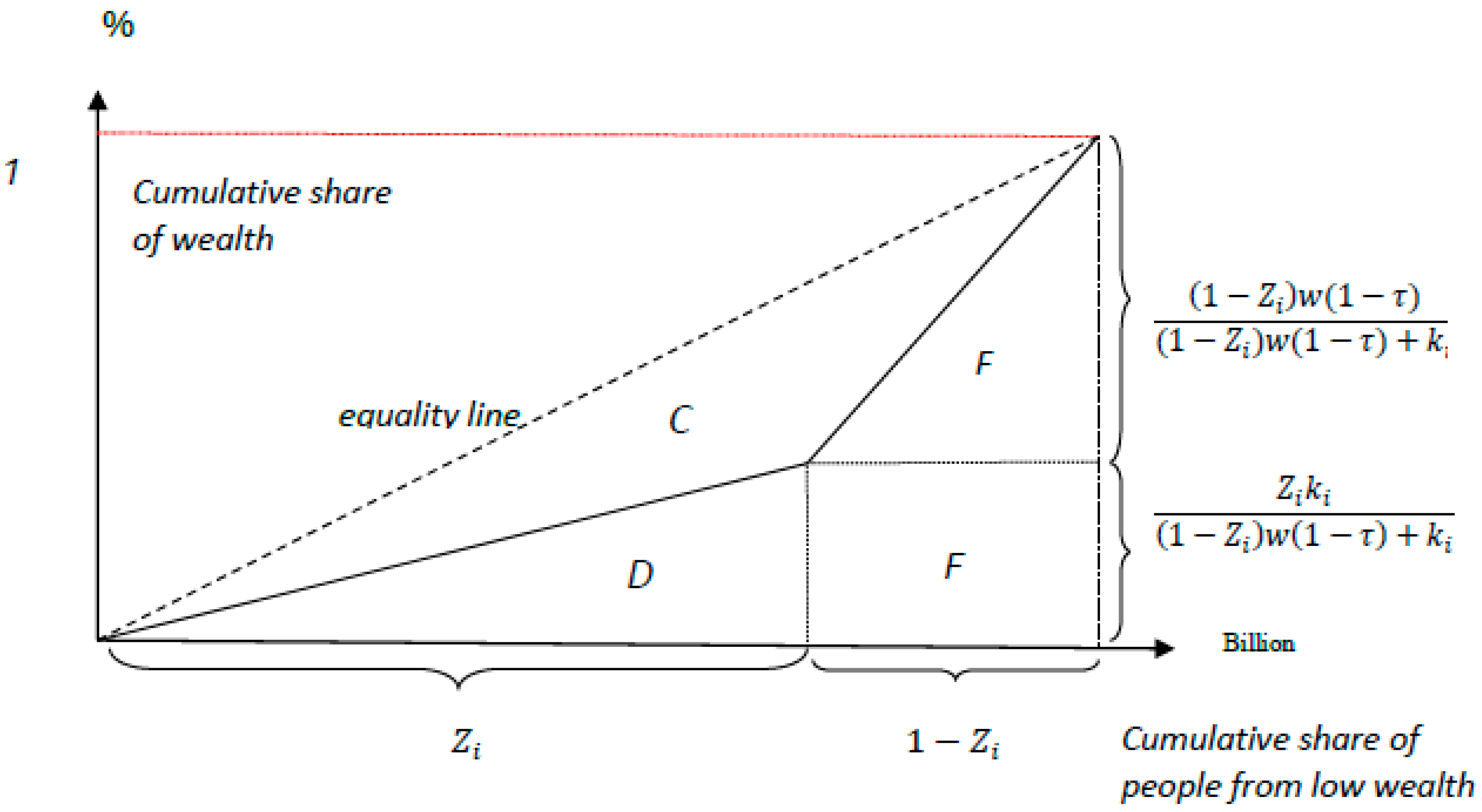
Note that tax revenues collected from the rich agents aggregate as $T_P=W\left(t\right)\tau$, that is, $\frac{T_P}{W\left(t\right)}=\tau$, where the rich agents’ wealth is denoted as $W\left(t\right)$, while the after-tax wealth of the rich is represented by the term $W\left(t\right)$ (1−τ). For the sake of simplicity, we assume $W\left(t\right)=w$. The proportion τ ∈ (0, 1) of the rich agents’ wealth w is taxed by the government and the tax revenue is collected and distributed within and across the rich in a lump-sum fashion. Thus, the after-tax and transfer wealth for the rich is $w$ (1−τ) + $k_i$, whereas that for the poor is $k_i$, where τ is the country-invariant billionaire tax rate and $k_i$ is the per capita lump-sum transfer that billionaire $i$ can hold in assets. The Gini coefficient is computed by C/C+(D+E+F) in Figure 2. Direct calculation gives the Gini index after tax as

$$Gini=\frac{Z_i}{1+\frac{k_i}{\left(1-Z_i\right)w\left(1-\tau \right)}}$$

(2)

For derivations of Equation (2) see Appendix A. Here, the numerator indicates the number of poor $Z_i$ while the denominator indicates the size of the redistribution $k_i$ (i.e., wealth of the poor), divided by the aggregate wealth of the rich, (1 − $Z_i$) w (1 − τ). A larger value of the numerator indicates a rise of income inequality between the rich and the poor, which accordingly leads to a higher Gini coefficient. Therefore, the assumption of $Z_i$ ∈ (0, 1) implies that the marginal cost of human capital investment is higher for the poor agents than the rich agents. That is, the wealthy individuals have a dominant position over poor individuals in being cultivated or skilled [33,34].

As more income goes to the rich, income inequality has a snowball effect on the wealth distribution. Thus, we can state the following proposition:

Proposition 1.

Both wealth and income are more concentrated among the wealthy individuals and will contribute to a higher Gini coefficient (i.e., income or wealth disparity).

For the proof, see Appendix B.

3.1.2. What Impact Does Raising Taxes on the Rich Have on Gini Indices?

As shown in Proposition 1, we focus on the relationship between wealth and inequality. Next, we consider how the effect of taxation on the rich agents’ wealth may contribute to reducing the inequality gap. Equation (2) also implicitly defines the Gini index before tax as

$$Gini=\frac{Z_i}{1+\frac{k_i}{\left(1-Z_i\right)w}}$$

(3)

Given this, we immediately obtain the following result with regard to the effect of redistributive taxation on inequality.

Proposition 2.

Given the condition (1 −$Z_i$) > 0, a higher redistributive tax rate leads to lower Gini inequality indices in terms of the after-tax-and-transfer wealth.

The proof is provided in Appendix C.

As stated in Proposition 2, the tax rate is negatively correlated with Gini indices when taking into account the effects of taxation on the wealthy, provided that there is some redistributive wealth variation. Building on this view, we also obtain the following Proposition:

Proposition 3.

When comparing pre- and post-tax Gini coefficients, the redistributive tax on the rich agents can contribute to lower wealth inequality (measured with Gini coefficients). In other words $G_1$ > $G_2$, where $G_1$, $G_2$ represent pre- and post-tax Gini coefficients, respectively.

Proof. 

Repeat the difference analysis carried out on the measure of Gini coefficients between Equations (2) and (3). The distribution of Gini differences is represented as the change of the Gini index between the pre-tax (G₁) and after tax (G₂) situations. Comparing the Gini coefficients yields:

$$G_2-G_1=G{i}_{diff}=\frac{Z_i}{1+\frac{k_i}{\left(1-Z_i\right)w\left(1-\tau \right)}}-\frac{Z_i}{1+\frac{k_i}{\left(1-Z_i\right)w}}=Z_i\left[\frac{1}{\frac{\left(1-Z_i\right)w\left(1-\tau \right)+k_i}{\left(1-Z_i\right)w\left(1-\tau \right)}}-\frac{1}{\frac{\left(1-Z_i\right)w+k_i}{\left(1-Z_i\right)w}}\right]$$

(4)

$$=Z_i\left[\frac{\left(1-Z_i\right)w\left(1-\tau \right)}{\left(1-Z_i\right)w\left(1-\tau \right)+k_i}-\frac{\left(1-Z_i\right)w}{\left(1-Z_i\right)w+k_i}\right]$$

(5)

$$\begin{array}{c}=Z_i\left[\frac{\left(1-Z_i\right)w\left(1-\tau \right)}{\left(1-Z_i\right)w\left(1-\tau \right)+k_i}-\frac{\left(1-Z_i\right)w}{\left(1-Z_i\right)w+k_i}\right]\\ =Z_i\left[\frac{\left(1-Z_i\right)w-\left(1-Z_i\right)w\tau }{\left(1-Z_i\right)w+k_i-w\tau \left(1-Z_i\right)}-\frac{\left(1-Z_i\right)w}{\left(1-Z_i\right)w+k_i}\right]\\ =w_{}{Z}_i\left[\frac{\left(1-Z_i\right)-\left(1-Z_i\right)\tau }{\left(1-Z_i\right)w+k_i/w-w\tau \left(1-Z_i\right)}-\frac{\left(1-Z_i\right)}{\left(1-Z_i\right)w+k_i/w}\right]\\ =w{\left(1-Z_i\right)}_{}{Z}_i\left[\frac{1-\tau }{\left(1-Z_i\right)w+k_i/w-w\tau \left(1-Z_i\right)}-\frac{1}{\left(1-Z_i\right)w+k_i/w}\right]<0\end{array}$$

(6)

since $<\tau \mathrm{and}w\tau \left(1-Z_i\right)<1$. □

The values of $\tau$, $w\tau \left(1-Z_i\right)$ in previous studies range from 0 [35] to 1 [36] because the values of $\tau$, $w\tau \left(1-Z_i\right)$ are less than 1. From Equations (4) to (6), it is clear that the calculated outcome induces the result that $Gin{i}_{diff}$ < 0, in contrast. Importantly, Equation (6) verifies that the Gini coefficient after the imposition of a billionaire tax is smaller than its value before the tax system and higher taxation reduces the Gini value.

3.2. Application to Numerical Computation of Gini

In this section, we seek to estimate Equation (2) and evaluate the calibration results of the theoretical model mentioned above.

The magnitude of the average human capital in the relevant literature is measured in the same way as Barro and Lee [37], ordering the units increasingly in terms of their average endowment of human capital. The parameters of the model for the numerical exercises in this study are set at standard values as $Z_i$ = 75 (human capital of the non-rich people) as applied in previous studies [38], where capital was interpreted broadly to include human capital baseline specifications, including values of $Z_i$ ranging from 0.85 to 0.9. Under the specified function based on Equation (2), we set the basic parameters as follows:

Taxes with variation parameters: $\tau$ is set in turn with alternative values as 0.1, 0.15, 0.2, 0.25, 0.3, 0.35, 0.4, 0.45 and 0.5. Note that the pre-tax values herein are regarded as the proxies before taxing billionaires.

Parameters setting: we measure wealth as $w$ values come from the below Forbes list of billionaires and $Z_i$ is set at 0.7, 0.8, 0.85 and 0.9 respectively. The labour income share $k_i$ is adopted as 0.75, which parameter setting can be found in [39,40].

3.2.1. Data on the World’s Billionaires

Traditional household income surveys do not accurately capture the wealth of the wealthiest, because of limits in coverage and/or the statistical significance of wealth inequality. Therefore, to consider the wealthiest class, we also analysed the effective income of billionaires from various nations and categorized them so that the income and other definitions would be precisely comparable, using the Forbes “The World’s Billionaires” ranking (see “The World’s Billionaires,” Forbes, 2015, www.forbes.com/billionaires/). Our data draw on global billionaires’ filings, showing that there was a record of 1826 billionaires, each with a reported net worth of more than $1 billion in 2015. The data provide more than $1 billion net worth records, representing unique billionaire tax filers and yielding census-scale evidence about the wealthiest people in the world. For simplicity, we refer to the billionaires under the tax burden as “billionaires.” While the term “billionaire” often connotes accumulated wealth, our focus is on the top percentile of incomes—those people who possess in recent years the most wealth that individuals have ever accumulated [41]. This paper presents new findings from the Global Billionaires Database and discusses some of their policy implications, both in terms of optimal tax policy and the interplay between inequality and global billionaires’ net worth.

3.2.2. Is Taxing the Wealthy a Good Policy Instrument for an Overall Decrease in Inequality?

How do top net worth shares relate to overall wealth inequality? Top wealth shares measure the concentration of pre-tax net worth of the top percentile in wealth distribution but they do not provide any information about the condition of the remaining parts of the wealth distribution. The Gini coefficients before taxes and transfers are positively related to the share of pre-tax income in the top percentile, albeit rather loosely (Figure 3). Lorenz curves are also shown in Figure 2 above, applied to both simulated and empirical data in this work.

The graphical overview of wealth ranking for the Gini index sheds light on asymmetry (skewness) and ultimately encompasses the stationary exponential shape depicted in Figure 3. Similarly, the stationary exponential shape distribution was found by Dragulescu and Yakovenko [42] to be asymmetric (skewed), with a shape qualitatively similar to the one shown in Figure 3. The Gini index’s pre-taxation curve is steeper and more downward trending than the original Gini index, suggesting that the sudden decline was partly due to tax-saving behaviour. Figure 3, Figure 4, Figure 5 and Figure 6 plot the additional cumulative distributions of wealth at stationary equilibrium from the cases of top marginal tax rates of τ = 0.5 to 0.1. Both wealth inequality and tax effects are considered by the extended Gini formula for global billionaires’ wealth. We observe that the Pareto exponents for wealth coincide, which explains why high-income people in this model acquire most of their income from accumulated wealth. Examining billionaires counted as the top 10 wealthiest people worldwide, the evidence reveals that the Gini coefficient is significantly smaller in high tax regimes than in low tax regimes: 0.72 for τ_min = 0.1 and 0.67 for τ_max = 0.5.

The low tax rate enhances the diffusion effect, because it increases the volatility of after-tax returns to wealth, while the low tax rate weakens the influx effect, because it reduces the net inflow of billionaires into the tail from below. Therefore, both effects induce a low Pareto exponent. As empirically studied by Feenberg and Poterba [43], an unprecedented decline in the Pareto exponent is observed immediately after tax reform. The steady Pareto exponent reduction in the 1990s could imply more persistent impacts of tax reform. Moreover, Piketty and Saez [44] also reported that the imposition of a progressive tax around World War II was a possible reason for the top income share remaining at a relatively low level for a long time, until the 1980s. Our simulations and the above analytical results of this paper are in agreement with the opinion that tax cuts substantially decrease the stationary Pareto exponent. Hereafter, while the top wealth shares do not imply anything about the middle and the bottom of the wealth distribution, the Gini coefficient is more sensitive to wealth variations in the top percentile than in the middle and in the tails of the distribution, because it reveals deviation from the mean or the spread of the wealth distribution. However, the impact of top wealth shares on post-tax and transfers of disposable wealth inequality are achieved via the government’s tax instrument, because the redistributive tax and transfer system typically decreases wealth disparities significantly. Changes in the top wealth shares do not systematically cause changes in overall inequality in terms of disposable wealth, while the redistributive impact of the tax system can change over time.

3.3.3. Numerical Results and Discussion

Table 1. Top percentile net worth shares and pre-, post -tax Gini coefficients of wealth inequality.

Rank	Pre-tax	τ = 0.5	τ = 0.45	τ = 0.4	τ = 0.35	τ = 0.3	τ = 0.25	τ = 0.2	τ = 0.15	τ = 0.1
1	0.763834	0.730796	0.736588	0.741486	0.745682	0.749316	0.752494	0.755297	0.7577	0.7600
2	0.762894	0.729078	0.735002	0.762894	0.744305	0.748025	0.751279	0.754149	0.7567	0.7589
3	0.760759	0.725187	0.731405	0.760759	0.741182	0.745095	0.74852	0.751543	0.7542	0.7566
4	0.756044	0.716667	0.723518	0.756044	0.734319	0.73865	0.742446	0.745799	0.7488	0.7515
5	0.74832	0.702913	0.710754	0.74832	0.723166	0.728161	0.732546	0.736427	0.7399	0.7403
6	0.735691	0.680952	0.690291	0.735691	0.705168	0.71119	0.716493	0.721198	0.7254	0.7291
7	0.735691	0.680952	0.690291	0.735691	0.705168	0.71119	0.716493	0.721198	0.7254	0.7291
8	0.733993	0.678049	0.687577	0.733993	0.702771	0.708925	0.714347	0.719159	0.7234	0.7273
9	0.732356	0.67526	0.684969	0.732356	0.700464	0.706745	0.712281	0.717196	0.7216	0.7255
10	0.731585	0.67395	0.683743	0.731585	0.69938	0.70572	0.711308	0.716271	0.7207	0.7247
Percentile threshold
Top 10%	0.62263	0.51482	0.53126	0.54588	0.55897	0.57076	0.58144	0.59116	0.60004	0.60819
Top 20%	0.54956	0.4273	0.44487	0.46079	0.47529	0.48857	0.50077	0.51203	0.52245	0.53213
Top 30%	0.49933	0.37337	0.39081	0.40680	0.42152	0.43513	0.44775	0.45949	0.47044	0.48069
Top 40%	0.46238	0.33651	0.35351	0.36921	0.38376	0.3973	0.40993	0.42175	0.43284	0.44327
Top 50%	0.42658	0.30296	0.31928	0.33445	0.3486	0.36184	0.37427	0.38595	0.39697	0.40738
Top 60%	0.40429	0.28298	0.29878	0.31352	0.32732	0.34028	0.35248	0.36399	0.37488	0.38519
Top 70%	0.37828	0.26055	0.27565	0.28981	0.30311	0.31565	0.3275	0.33871	0.34935	0.35947
Top 80%	0.35739	0.24318	0.25766	0.27128	0.28412	0.29625	0.30775	0.31866	0.32904	0.33893
Top 90%	0.33669	0.22644	0.24027	0.25332	0.26565	0.27733	0.28843	0.29899	0.30906	0.31868

Notes: 1. Empirical specification of wealth Gini; 2. Distribution characteristics in the model and among global billionaires. The table lists quintiles of wealth $w_i$, Gini index of wealth and the top ranked 10-th in wealth is measured relative to the top 90% share of wealth.

presents the estimation results for the Gini indices among wealth holders from the global billionaires under various tax rate regimes. We conduct a proper sensitivity analysis using a simulation approach to find that the changes in the parameter values can determine the fluctuations in the distribution. In Table 1, the Gini index illustrates an increasing trend in the case of lower tax rates. Thus, a decrease in τ has exactly the same result as a cut in Gini incise does. The billionaire tax also lowers net worth; equalization of wealth dominates the effects and the overall inequality measurement, that is, the Gini coefficient, decreases. Figure 3, Figure 4, Figure 5 and Figure 6 show the Gini coefficient for each distribution. The graphs display that the fit is quite good. The evaluated coefficient varies remarkably as the parameter changes. The plausible range of fluctuations of the model parameters can cover the range of Gini coefficients observed in the data. Additionally, we examine whether the impacts of our fundamental parameters $Z_i$ and $k_i$ on the Gini coefficients demonstrate statistical significance in the various tax rate data. The agreement between the post-tax model and the pre-tax model, with convexity constraints, indicates the key roles played by the influx effect and the diffusion effect in yielding Pareto distribution. The most striking result that we found is the almost total decay of the high-wealth class, while in all other scenarios of Gini indices or Gini index criteria post-tax, the high-wealth class is quite robust, despite the financial markets’ turbulence.

4. Taxation, Inequality and CSR: Empirical Study

Given our emphasis on financial markets, our study has parallels in the relevant literature on the impacts of capital gains taxes. In previous research, Fischer and Jensen [7] also studied the effects of redistributive taxation on stock prices. In elaborating their model, which is similar to ours, tax revenue is exposed to stock market risk. However, their model included only one risky asset (and thus no idiosyncratic risk) and output did not depend on taxation and thus originated from a Lucas tree. Studies of inequality in asset prices, using frameworks very different from ours, have included Favilukis [10] as well as Pástor and Veronesi [45]. More broadly, our study is related to the relevant literature on income inequality with quantile regression approaches and we add an endogenous agent type selection, that is, compensation indicator variables and block trade shocks to Gini indices. Moreover, we focus on stock market participation, wealth inequality and the HC index. Indeed, risky real assets, including capital gains, equity holdings and investment securities, contribute the major components, with the greatest proportional factors to income inequality, making a contribution of more than 50 percent for many years. Capital gains on stocks and stock holdings, in other words, are key factors necessary to emphasize the growing importance of risky financial assets and they show changes in inequality consistent with those in net worth [8,10]. Hence, the flowing hypothesis can be advanced:

Hypothesis 1 (H1).

Block trading securities show significant differences in amount (or volume) before and after the 2015 abolition of capital gains taxation.

4.1. Hypotheses Regarding Inequality and Welfare Improvement of CSR

Building on the above theoretical discussions in the relevant literature section, regarding the effect of economic inequality between the wealthy agents and CSR indicators, we now formulate the following three hypotheses for empirical testing in this section.

Hypothesis 2 (H2).

The HC (a reliable indicator of CSR in the model) with the higher index will have larger Gini indices and lower welfare values.

Hypothesis 3 (H3).

Block holders of stock trading at higher volume levels will expand wealth inequality as well as income inequality, also when controlling for welfare conditions. Importantly, these two hypotheses do not exclude the possibility of feedback from inequality to CSR indicators. On the contrary, the links reviewed suggest that:

Hypothesis 4 (H4).

Blockholders’ amount of stock trade increases market inequality, given a sufficient signal as the representative wealthy agents’ behaviour, while for net inequality theoretical expectations are ambiguous.

4.2. Econometric Specification

To provide some robust findings about the role of the rich agents’ wealth in the inequality–CSR relationship from Equation (2), we obtain:

$$\mathbb{G}ini=\frac{Z_i}{1+\frac{k_i}{\left(1-Z_i\right)W}}=\frac{Z_i\left(1-Z_i\right)W}{\left(1-Z_i\right)W+k_i}$$

(7)

This study adds CSR activism to the model and the following empirical specification is formulated:

$$\widehat{Gini}=\widehat{G}=\frac{Z_i\left(1-Z_i\right)W}{\left(1-Z_i\right)W+k_i}+\gamma CSR$$

(8)

Via Equation (8), the model hypothesizes that wealth inequality is determined by two main variables of interest, namely the rich agents’ wealth and CSR activities and their interaction, captured as a set of other control variables. Equation (8) also implicitly defines the Gini decomposition $\widehat{G}$ as a function of the representative wealth variables and $CSR$ with $\gamma$.

4.3. Sample Selection

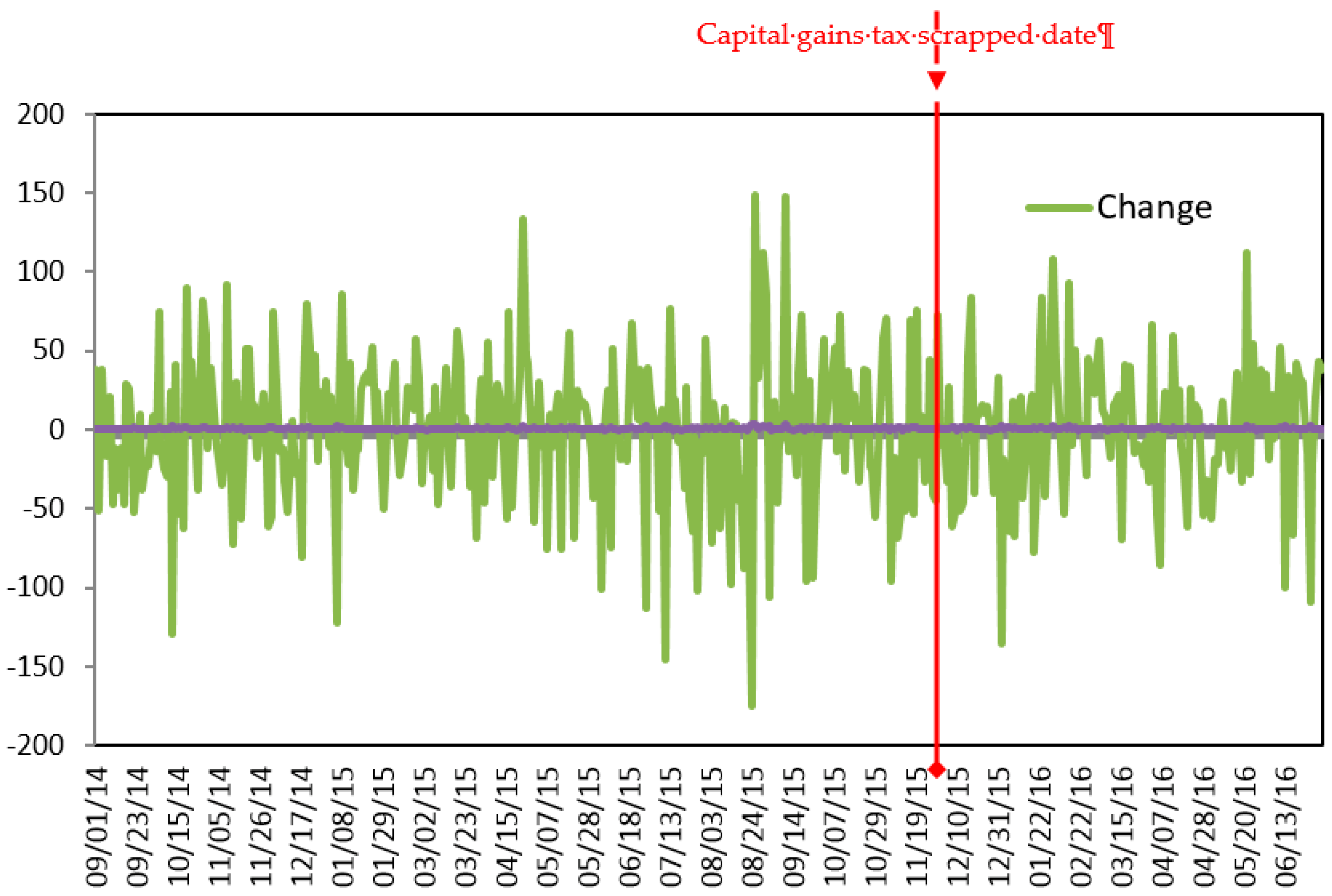
A wealthy investor is one who has the capability to engage in large-block transactions. The impact of block trades is a proxy behaviour for the wealthy and for appropriate decompositions of inequality indices. The sample consists of the daily quotes of block trade securities and the Taiwan High Compensation 100 Index (HC 100) covering the period from September 1, 2014, to June 30, 2016 and the sample extends its period to the date on which the 2015 capital gains tax was scrapped. The method for matching the block trades shows that the transactions were executed according to the terms of the prices quoted and the volumes by the buyer and the seller. In addition, we can examine the daily trading volume impact of block trade types of traders on the market and calculate the capital gains tax effects. Various measurements of size, including the number of shares traded, the natural logarithm of the dollar value of the trade and the volume relative to average daily trading volume, are tested. Overall, the natural logarithm of the larger-sized trades provides the best fit for the model. Block trades are expected to be linked to greater wealth impacts. Finally, we employ block trades measured by the TSE market for the portfolios of the wealthy to capture their behaviour [11], which is accomplished by first computing the holdings of the block shareholders with bid–ask block trade types from the wealth distribution. Taken together, based on the empirical evidence in this study, we attempt to analyse the high compensation group incorporated with one of the CSR indices, using the HC100 index. In conclusion, the above selected measures of sample indices and their corresponding variables are listed in Appendix D (

Table A1. The selected measures, Variable or Criteria Definitions and Sources.

Variable	Definition	Dimension	Source	Sample period
$Gini$	$Gini$ index represents Inequality indicator	Economic	Own calculations based on the WIID	1963–2016
$Volume$	The stock trading volumes in block size of stock holdings	Economic	Taiwan Stock Exchange (TWSE)	Sep.1, 2014–June 30, 2016.
$Amoun{t}_{}$	The stock trading amount in block size of stock holdings that is, $Block$ $Trade$	Economic	Taiwan Stock Exchange (TWSE)	Sep. 1,2014–June 30, 2016.
$HCindex$	$Highcompensationindex$ denotes CSR activities.	Social	Taiwan HC 100 Index (TWSE)	Sep. 1, 2014–June 30, 2016.

Notes: Gini index refer to WIID—the World Income Inequality Database: https://www4.wider.unu.edu.

).

4.4. Empirical Methodology and Strategy

4.4.1. Testing the Above Hypotheses

Following from Equation (8), to examine variations in the magnitude of the wealth inequity impact of block trades, the main econometric specification is:

$$ln{\left(Gini\right)}_{inequalityimpact}^{}=c+{\alpha }_{1}ln\left(Volum{e}_{BlockTrade}\right)+{\alpha }_{2}ln(Amoun{t}_{BlockTrade})+\beta ln\left(HCindex\right)+\epsilon$$

(9)

where Volume _{Block Trades}, Amount _{Block Trades} proxy for the wealthy people’s behaviour, representing stock trading volumes and amounts in the block size of stock holdings, respectively. Notably, HC index as a proxy for CSR indicator is also related with high income earners. The Gini values illustrated in Table 1 are selected for the closest fit to Taiwan’s historical data distributions, in such a way that the whole range of possible averages to the Gini algorithm (depicted in Equation (2)) is represented.

4.4.2. Empirical Strategy

The capital gains are obtained from the risky bid–ask equity in the stock market and they contribute to income inequality. To overcome the problem of extreme values caused by economic inequality, we use a variant of the counterfactual decomposition methodology employed by quantile regression [8,46]. The conditional distribution of $\mathcal{Y}$ allows for regressor $X$ as follows:

$$Q_n(\theta |{\mathcal{Y}}_i,b\left(\theta \right))=X_i^{\prime }b\left(\theta \right)$$

(10)

where parameter $b\left(\theta \right)$ can be estimated and the specification nexus between vector $X$ and $\theta$ the conditional quantile of the variable $\mathcal{Y}$ are determined by Equation (10). Then, by minimizing the weighted absolute residuals from the conditional quantile, the parameters can be estimated as follows:

$${\widehat{b}}_{\theta }=argminE\left[I_{\theta }\left({\mathcal{Y}}_i-X_i^{’}b\right)\right]Q_n$$

(11)

where the dependent variable ${\mathcal{Y}}_i$ is governed by different $\theta$th quantiles given $X_i$ and $I_{\theta }$ denotes a weighting check function, which shows positive and negative deviations asymmetrically for any $\theta$ ∈ (0, 1). The indicator function can be adapted and yields

$$I_{\theta }\left({\xi }_i\right)=\left\{\begin{array}{cc}\theta {\xi }_i\hfill & \hfill if\xi {}_i\ge 0\\ \left(1-\theta \right)\xi {}_i\hfill & \hfill if\xi {}_i<0\end{array}\right\}$$

(12)

where ${\xi }_i={\mathcal{Y}}_i-X_i^{\prime }b$, then Equations (11) and (12) illustrate that

$${\widehat{b}}_{\theta }=argmin\left(\begin{array}{cc}{\displaystyle \sum }_{{\mathcal{Y}}_i>X_i^{\prime }b}\theta \left|{\mathcal{Y}}_i-X_i^{\prime }b\right|+& {\displaystyle \sum }_{{\mathcal{Y}}_i<X_i^{\prime }b}\left(1-\theta \right)\left|{\mathcal{Y}}_i-X_i^{\prime }b\right|\end{array}\right)=argmin\left\{{{\displaystyle \sum }}_i{I}_{\theta }\left[{\mathcal{Y}}_i-X_i^{\prime }b\left(\theta \right)\right]\right\}$$

(13)

where Equation (13) indicates that optimization via minimizing the sum of weighted absolute residuals determines the quantile regression estimators.

5. Empirical Findings

Table 2. Summary statistics.

	Full Sample					Pre-ACGT Period (3 September 2014–17 November 2015)			Post- ACGT Period (18 November 2015–30 June 2016)
	Panel A: Descriptive Statistics of Variables
	Mean	Median	S.D.	Min.	Max.	Mean	Median	S.D.	Mean	Median	S.D.
Gini	0.357	0.346	0.067	0.269	0.52
HC_Index	4860.476	4824.15	303.794	4141.53	5511.53	4834.25	4814.69	301.19	4889.15	4863.98	309.078
Amount	1184.273	902.56	1057.085	18.088	10,084.82	1192.992	907.71	1077.71	1166.891	901.04	1018.04
Volume	24.626	17.411	30.294	0.119	326.311	23.517	28.788	28.788	26.837	33.083	33.083
Test for equality of means between two series (pre-and post-ACGT periods)
	t-test	Welch t-test P-value
HC_Index	0.361	0.351		0.705
Amount	0.246	0.251		0.805
Volume	−1.095	−1.046		0.273
	Panel B: Breakpoint Test: 11/18/2015 Null Hypothesis: No breaks at specified breakpoints
	Chow Breakpoint Test Quandt-Andrews unknown breakpoint test
	F-statistic	Wald Statistic		Prob.		F-statistic	Wald Statistic		Prob.
HC_Index	0.637	1.27		0.53		2.71	1.408		0.24
Amount	0.518	0.52		0.4721		1.675	1.68		0.3
Volume	1.329	1.33		0.2494		2.5166	1.333		0.145

Notes: 1. This table provides summary statistics for the mean, standard deviation and 50th percentile of all variables used in the following regression model for the entire sample, as well as for separate subsamples. 2. There are 4 variables surrounding each accompanied with 449 observations. Amount and Volume are in millions of NT$ and shares, respectively. 3. ***, **, * indicate that the variables are different between the pre- and post- ACGT periods at the 1%, 5% and 10% levels of significance, respectively. 4. Panel A reports the usual summary statistics. Panel B reports the Chow and Quandt-Andrews tests for the pre- and post- ACGT periods we consider.

depicts a summary of statistics showing the main variables’ characteristics for the full sample and the sub-samples before and after abolishing capital gains taxation (ACGT). Panel A of Table 2 shows ordinary sample statistics, while Panel B, in order to reduce the potential effects of structural breakpoint, presents the Chow and Quandt-Andrews tests for the pre- and post-ACGT periods we consider.

5.1. Testing for Structural Breaks Before and After the ACGT

As a robustness test, we turn our attention to two widely used tests that are adopted in testing for structural breaks in econometric models. Both Chow’s and Quandt-Andrews’ tests (depicted as Panel B of Table 2) show that there is no significant breakpoint for the entire sample and the sub-samples for the pre- and post-ACGT periods. In summary, the findings indicate the capital of block trade volumes and amount in the stock market outflow to overseas investment. The results indicate that there is no significant change in the estimates of the pre-ACGT amount and volume sensitivities and their changes post-ACGT in block trade stocks. Hence, assumption H₁ is not validated. This is consistent with our findings as depicted in Figure 7, Figure 8 and Figure 9. We find this to be in contrast with Meh [47], who demonstrated that the elimination of progressive taxation has a negligible effect on wealth inequality where entrepreneurship is concerned but has a great effect when the entrepreneurship variable is omitted.

5.2. Does Taxation of the Wealthy or Its Indicator of Usage Matter to Income Inequality Governance?

Equity holdings illustrate one of the highest ranks resulting in wealth disparity, increasing over time and emphasizing the growing importance of risky financial assets in the overall net wealth distribution, while a positive stock market return increases inequality, because it primarily benefits a disproportionate distribution to the wealthy [10]. Net worth inequality has followed the same trajectory, while stock wealth inequality over the period and stock wealth inequality have grown significantly, playing an important role as a component of net wealth inequality. All in all, we find no evidence that either block trades on stock wealth or overall net worth inequality decreased consistently through the period of capital gain tax elimination in the Taiwan stock market. Importantly, to narrow the gap between rich and poor, a proposal to tax some capital gains from the stock market was passed by the legislature in the middle of 2013 in Taiwan. The volatility and price impact of the Taiwan HC100 Index and the transaction amount volume in block trades are examined by capital gains tax shocks. Obviously, using the graphs shown overall in Figure 7, Figure 8 and Figure 9, there is no significant difference before or after the capital gains tax is scrapped throughout the period under examination. The impact of the growth of block trades and the Taiwan HC100 index in TAIEX market were not found anywhere else after the capital gains tax was scrapped and the capital gains tax policy was a failure in Taiwan.

5.3. The Changes in Inequality and Their Relation to CSR Activities

The impact of block trades is a proxy behaviour for the wealthy and appropriate decompositions of the inequality index are provided to study the relative importance of various asset components of net worth in generating wealth disparities. Inequality in a variable Gini can be expressed as the exact sum of the contributions made by its various factor components. In what follows, the top wealth distribution, which accounts for the main bulk of corporate equity holdings, is considered to use the amount and volume in block trades. Finally, the Gini index records a slight increase in net wealth inequality over time. The Gini indices might be more appropriate measures of inequality, because they capture the various quantiles of shareholder distribution and are especially sensitive to variation in the upper quantiles.

Table 3. Quantile Regression and Coefficient Estimates for the Impact of Inequity (Gini).

Variable	0.25	t-Statistic	0.5	t-Statistic	0.75	t-Statistic	0.9	t-Statistic	0.95	t-Statistic
ln HC index	1.185	17.456 *** (0.000)	1.24	11.954 *** (0.000)	1.699	9.93 *** (0.000)	2.36	18.48 *** (0.000)	2.5	22.06 *** (0.000)
ln VolumeBlock Trades	−0.011	1.043 (0.297)	0.002	0.201 (0.84)	0.024	0.858 (0.39)	0.04	2.13 ** (0.033)	0.055	2.82 *** (0.005)
ln AmountBlock Trades	−0.0002	−0.02 (0.983)	−0.007	−0.674 (0.5)	−0.029	−1.363 (0.173)	−0.022	−0.968 (0.33)	−0.033	−1.655 (0.11)
Cons	−4.034	−15.972 ***	−4.22	−11.32 ***	−5.82	9.155 ***	−8.323	−18.21	−8.73	−21.458 ***
Adjusted R-squared	0.278		0.264		0.189			0.212	0.18
Quasi-LR statistic	246.14		47.8		92.42			94.07	68.33
Prob (Quasi-LR stat)	<0.01		<0.01		<0.01			<0.01	<0.01

Notes: 1. We use ***, ** and * to denote significance at the 1%, 5% and 10% levels, respectively. The p-values reported in parentheses. 2. The Table presents the 0.25, 0.50, 0.75, 0.9 and 0.95 quantile regression coefficient estimates.

illustrates decompositions of inequality by source, as measured by the block transactions and the HC100 index. The coefficients ${\alpha }_1$ of the volumes of block equity trading (ln Volume _{Block Traes}), which proxy for the wealth inequality component, are positive and significant for the 90th and 95th percentiles at the 0.05 level for the Gini indices (ln Gini) Stock market participants are, on average, wealthier and gain disproportionately from stock market booms. Indeed, the present study did not find evidence that block trades in amount (ln Amount_{Block Trades}) are associated with variations in inequality indices at all percentiles. Thus, the evidence of the preceding two results supports hypotheses H3 and H4, respectively. More precisely, the positive coefficients $\beta$ of the Taiwan HC100 index (ln HC) evaluated at various percentiles have a statistically significant influence on Gini indices (ln Gini). Table 3 also displays decompositions of inequality in net total wealth, as summarized by the coefficient, which is applied to roughly match the rise in participation, the rise in the Taiwan HC100 index and the increase in Gini index, that is, the rise in income inequality and its impact is significant. Thus, hypothesis H2 is supported. Our empirical investigation suggests that the movement in the HC index dominated the expansion of the stockholder base in determining the overall outcome for Gini indices, which links stockholding participation directly to indicators of financial concentration (wealth inequality). In some cases, the adjusted R-squared value in time series data should not be the major measure of the predictive power statistics for regression models. Checking a model for fitting adequacy focuses on the relative rather than the absolute, therefore, the best way would be to consider other regression models. More precisely, we also have applied the following cointegration regression to check the robustness of our estimated results.

5.4. Robustness of Results in the Cointegration Analysis

In the interest of checking the property of the main variables, as depicted in

Table 4. ADF and Phillips-Perron Unit Root Test Results (in Levels and Differences).

Variables	Unit Root Test
Level	ADF	Prob.	PP	Prob.	Result
	Z-statistics		Z-statistics
ln HC	-	0.5506	-	0.5016	I (0)
ln Volume	-	0.5655	-	0.0112	I (0)
ln Amount	-	0.6026	-	0.4243	I (0)
cross-sections	−1.65526		−6.55
First Difference
ln HC	-	0.0000 *	-	0.0000 *	I (1)
ln Volume	-	0.0000 *	-	0.0001 *	I (1)
ln Amount	0.0000 *		0.0001 *		I (1)
cross-sections	−10.60		−16.73

Note: 1. * denotes the significance level at 1%. 2. Z-statistics is three cross-sections included and denotes Choi Z-statistics Choi [51].

, the empirical results using unit root tests reveal that the main variables are integrated to first order and display the property of being I (1). To check the robustness of the above evidence, the Johansen cointegration analysis is performed to identify the existing cointegrating relationship (

Table 5. Johansen cointegration test results (continued).

Hypothesized		Trace	0.05
No. of CE(s)	Eigenvalue	Statistic	Critical Value	Prob. **
None *	0.142040	152.6374	47.85613	0.0000
At most 1 *	0.099604	84.61783	29.79707	0.0000
At most 2 *	0.074203	38.03319	15.49471	0.0000
At most 3	0.008524	3.800727	3.841466	0.0512

Notes: 1. Trace test indicates 3 cointegrating equations at the 0.05 level. 2. * denotes rejection of the hypothesis at the 0.05 level. 3. ** represents p-values of MacKinnon-Haug-Michelis [52].

). Hereafter, let Equation (9) be transformed to the forms specified below and the further cointegrating regression may refer to the fully modified ordinary least squares regression (FMOLS) technique of Phillips and Hansen [48], the dynamic ordinary least squares (DOLS) approach of Stock and Watson [49] and the conical cointegration regression (CCR) of Park [50], respectively. These econometric methodologies provide a robustness check of estimates able to yield reliable results when the sample size is small. As can be seen in

Table 6. Long-run relationship for the dependent variable of Gini index.

Dependent Variable: ln Gini
Variables	FMOLS p-Value	DOLS p-Value	CCR p-Value
ln HC	1.565 [0.0001 *]	1.551 [0.0001 *]	1.511 [0.0005 *]
	(6.976)	(18.993)	(3.495)
ln Volume	0.019 [0.498]	0.027 [0.1655]	0.191 [0.0057 *]
	(0.681)	(1.389)	(2.778)
ln Amount	−0.028 [0.3372]	−0.0418 [0.0174]	−0.139 [0.0325]
	−0.960	−2.387	−2.145
Constant	−5.5352 [0.0001 *]	−5.269 [0.0001 *]	−5.0565 [0.0024 *]
	(−6.528)	(−18.548)	(−3.053)
S.E. of regression long-run variance	0.053 0.016	0.0528 0.015	0.0706 0.0983

Notes: 1. * represents the significance level at 1%. The value in the parentheses and square brackets are T-statistics and p-value, respectively. 2. Long run variance estimate is expressed as Newey-West fixed bandwidth 4.0. 3. Cointegrating equation deterministic: Constant, Trend.

, the models obtained by using the FMOLS and CCR techniques were found to produce similar outcomes to the evidence examined in Table 3. In conclusion, using three alternative estimators, FMOLS, DOLS and CCR cointegration tests, the empirical findings demonstrate a significant long-run relationship between the income inequality and block trade of stockholding along with CSR indicators.

6. Conclusions, Limitations and Policy Implications

To conclude, in the present paper we provided for the first time a comparison of wealth inequality in pre-tax and post-tax scenarios and therefore the redistribution achieved by the government through taxes. This was possible because we applied and extended Yakovenko and Rosser’s [53] formalism. The transition path in the simulated model is consistent with the top share of wealth increasing after the tax cut, since aggregate capital and the top wealth shares converge to a new stationary level relatively quickly. This paper investigates the empirical shape of wealth distribution with a parametric specification motivated by the basic fact that wealth inequality is derived from an extended Gini index formula. Importantly, the tax code for the wealthy serves as the economic backdrop for sustainable CSR activities. This paper further proposes an HC index by studying the role of block trades in stock structures and the role of governance systems in shaping corporate social responsibility for upper-income groups.

6.1. Limitations for Future Research

This paper focused on identifying the CSR activity of high-income groups, although facing some limitations: issues such as tax evasion and tax compliance were not considered. In addition, some interesting issues (e.g., more CSR indicators) could be discussed. For further research, CSR activism aimed at increasing tax compliance in wealthy individuals should be examined. Similarly, the findings obtained from this study can be compared with the results of block trading with stakeholder engagement present in companies’ CSR reports to extend the discussion of CSR. However, we leave the deeper empirical analysis of this issue to future researchers.

6.2. Policy Implications

Among the potential caveats of this study’s findings lie four stylized facts: (1) the 2015 ACGT policy does not work in Taiwan due to capital flight; (2) when tax rates for the wealthy are increased, wealth inequality declines; (3) a higher HC index predicts greater Gini indices; and (4) the share of wealth invested in equity increases sharply at the top of the wealth distribution. Two broader interpretations of these results associated with inequality governance policy are as follows:

First, on the theoretical side, taxation for the wealthy explains the decline in inequality, as captured by the Gini indices. On the empirical side, many challenges are involved in taxation practice. For example, there is no significant change between the pre- and post-ACGT periods in Taiwan’s block trade stocks. On the other hand, our findings also indicate that the HC index has a significant effect on Gini indices but block trading does not. Thus, the HC index is a statistically significant predictor of Gini indices through the channels just described. According to this view, an income-inequality governance perspective offers a fruitful research strategy for CSR scholarship. Accordingly, tax policy is not the only channel for reducing wealth inequalities. Other policies can directly support middle-class incomes, such as access to incentivizing compensation policies or more general CSR activism.

References

- Piketty, T. Capital in the Twenty-First Century; Harvard University Press: Cambridge, MA, USA, 2014. [Google Scholar]
- Volscho, T.W.; Kelly, N.J. The rise of the super-rich: Power resources, taxes, financial markets and the dynamics of the top 1 percent, 1949 to 2008. Am. Sociol. Rev. 2012, 77, 679–699. [Google Scholar] [CrossRef]
- Quadrini, V. The importance of entrepreneurship for wealth concentration and mobility. Rev. Income Wealth. 1999, 45, 1–19. [Google Scholar] [CrossRef]
- Cagetti, M.; De Nardi, M. Entrepreneurship, frictions and wealth. J. Political Econ. 2006, 114, 835–870. [Google Scholar] [CrossRef]
- Cagetti, M.; De Nardi, M. Estate Taxation, Entrepreneurship, and Wealth. American Econ. Rev. 2009, 99, 85–111. [Google Scholar] [CrossRef] [Green Version]
- Roussanov, N. Diversification and its discontents: Idiosyncratic and entrepreneurial risk in the quest for social status. J. Financ. 2010, 65, 1755–1788. [Google Scholar] [CrossRef]
- Fischer, M.; Jensen, B.A. Taxation, transfer income and stock market participation. Rev. Financ. 2015, 19, 823–863. [Google Scholar] [CrossRef]
- Bilias, Y.; Georgarakos, D.; Haliassos, M. Has greater stock market participation increased wealth inequality in the US? Rev. Income Wealth 2017, 63, 169–188. [Google Scholar] [CrossRef]
- Benhabib, J.; Bisin, A.; Zhu, S. The distribution of wealth and fiscal policy in economies with finitely lived agents. Econometrica 2011, 79, 123–157. [Google Scholar]
- Favilukis, J. Inequality, stock market participation and the equity premium. J. Financ. Econ. 2013, 107, 740–759. [Google Scholar] [CrossRef]
- Alzahrani, A.A.; Gregoriou, A.; Hudson, R. Price impact of block trades in the Saudi stock market. J. Int. Financ. Mark. Inst. Money 2013, 23, 322–341. [Google Scholar] [CrossRef] [Green Version]
- Ashbaugh-Skaife, H.; Collins, D.W.; LaFond, R. The effects of corporate governance on firms’ credit ratings. J. Acc. Econ. 2006, 42, 203–243. [Google Scholar] [CrossRef] [Green Version]
- Bhojraj, S.; Sengupta, P. Effect of corporate governance on bond ratings and yields: The role of institutional investors and the outside directors. J. Bus. 2003, 76, 455–475. [Google Scholar] [CrossRef]
- Hong, B.; Li, Z.; Minor, D. Corporate governance and executive compensation for corporate social responsibility. J. Bus. Ethics 2016, 136, 199–213. [Google Scholar] [CrossRef]
- Shleifer, A.; Vishny, R.W. A survey of corporate governance. J. Financ. 1997, 52, 737–783. [Google Scholar] [CrossRef]
- Jackson, G.; Apostolakou, A. Corporate social responsibility in Western Europe: An institutional mirror or substitute? J. Bus. Ethics 2010, 94, 371–394. [Google Scholar] [CrossRef]
- Ioannou, I.; Serafeim, G. The impact of corporate social responsibility on investment recommendations: Analysts’ perceptions and shifting institutional logics. Strateg. Manag. J. 2015, 36, 1053–1081. [Google Scholar] [CrossRef]
- Young, C.; Varner, C. Millionaire migration and state taxation of top incomes: Evidence from a natural experiment. Natl. Tax J. 2011, 64, 255–283. [Google Scholar] [CrossRef]
- Kim, J.; Im, C. Study on Corporate Social Responsibility (CSR): Focus on Tax Avoidance and Financial Ratio Analysis. Sustainability 2017, 9, 1710. [Google Scholar] [CrossRef]
- Gulzar, M.; Cherian, J.; Sial, M.S.; Badulescu, A.; Thu, P.A.; Badulescu, D.; Khuong, N.V. Does Corporate Social Responsibility Influence Corporate Tax Avoidance of Chinese Listed Companies? Sustainability 2018, 10, 4549. [Google Scholar] [CrossRef]
- Kacperczyk, M.; Nosal, J.B.; Stevens, L. Investor Sophistication and Capital Income Inequality; NBER Working Paper Series No. 20246; NBER: Cambridge, MA, USA, 2014. [Google Scholar]
- Guo, H. Limited stock market participation and asset prices in a dynamic economy. J. Financ. Quant. Anal. 2004, 39, 495–516. [Google Scholar] [CrossRef]
- Guvenen, F. Do stockholders share risk more effectively than non-stockholders? Rev. Econ. Stat. 2007, 89, 275–288. [Google Scholar] [CrossRef]
- Hungerford, T. Changes in income inequality among U.S. tax filers between 1991 and 2006: The role of wages, capital income, and taxes. SSRN 2013. [Google Scholar] [CrossRef]
- Roine, J.; Waldenström, D. On the role of capital gains in Swedish income inequality. Rev. Income Wealth 2012, 58, 569–587. [Google Scholar] [CrossRef]
- Jamali, D.; Safieddine, A.M.; Rabbath, M. Corporate governance and corporate social responsibility synergies and interrelationships. Corp. Gov. Int. Rev. 2008, 16, 443–459. [Google Scholar] [CrossRef]
- Flammer, C.; Hong, B.; Minor, D. Corporate governance and the rise of integrating CSR criteria in executive compensation. Acad. Manag. Proc. 2017, 1. [Google Scholar] [CrossRef]
- Berrone, P.; Gomez-Mejia, L. Beyond financial performance: Is there something missing in executive compensation schemes? In Global Compensation: Foundations and Perspectives; Gomez-Mejia, L., Wenner, S., Eds.; Routledge: New York, NY, USA, 2008; pp. 206–218. [Google Scholar]
- Jo, H.; Harjoto, M.A. Corporate governance and firm value: The impact of corporate social responsibility. J. Bus. Ethics 2011, 103, 351–383. [Google Scholar] [CrossRef]
- Pryce, A.; Kakabadse, N.K.; Lloyd, T. Income differentials and corporate performance. Corp. Gov. 2011, 11, 587–600. [Google Scholar] [CrossRef]
- Miles, P.C.; Miles, G. Corporate social responsibility and executive compensation: Exploring the link. Soc. Responsib. J. 2013, 9, 76–90. [Google Scholar] [CrossRef]
- Cai, Y.; Jo, H.; Pan, C. Vice or virtue? The impact of corporate social responsibility on executive compensation. J. Bus. Ethics 2011, 104, 159–173. [Google Scholar] [CrossRef]
- Blumkin, T.; Sadka, E. Income taxation with intergenerational mobility: Can higher inequality lead to less progression? Eur. Econ. Rev. 2005, 49, 1915–1925. [Google Scholar] [CrossRef]
- Hassler, J.; Mora, J.V.R.; Zeira, J. Inequality and mobility. J. Econ. Growth 2007, 12, 235–259. [Google Scholar] [CrossRef]
- King, R.G.; Rebelo, S. Public policy and economic growth: Developing neoclassical implications. J. Political Econ. 1990, 98, S126–S150. [Google Scholar] [CrossRef]
- Mendoza, E.G.; Milesi-Ferretti, G.M.; Asea, P. On the ineffectiveness of tax policy in altering long-run growth: Harberger’s superneutrality conjecture. J. Public Econ. 1997, 66, 99–126. [Google Scholar] [CrossRef]
- Barro, R.J.; Lee, J.-W. Sources of economic growth. Carnegie-Rochester Conf. Ser. Public Policy 1994, 40, 1–46. [Google Scholar] [CrossRef]
- Barro, R.J.; Sala-i-Martin, X. Convergence. J. Political Econ. 1992, 100, 223–251. [Google Scholar] [CrossRef] [Green Version]
- Gali, J. Government size and macroeconomic stability. Eur. Econ. Rev. 1994, 38, 117–132. [Google Scholar] [CrossRef]
- Lawless, M.; Whelan, K.T. Understanding the dynamics of labour shares and Inflation. J. Macroecon. 2011, 33, 121–136. [Google Scholar] [CrossRef]
- Keister, L.A. The one percent. Ann. Rev. Sociol. 2014, 40, 347–367. [Google Scholar] [CrossRef]
- Dragulescu, A.; Yakovenko, V.M. Statistical mechanics of money. Eur. Physical J. B 2000, 17, 723–729. [Google Scholar] [CrossRef] [Green Version]
- Feenberg, D.R.; Poterba, J.M. Income inequality and the incomes of very high-income taxpayers: Evidence from tax returns. In Tax Policy and the Economy; Poterba, J.M., Ed.; MIT Press: Cambridge, MA, USA; London, UK, 1993; Volume 7, pp. 145–177. [Google Scholar]
- Piketty, T.; Saez, E. Income inequality in the United States, 1913–1998. Q. J. Econ. 2003, 118, 1–39. [Google Scholar] [CrossRef]
- Pástor, L.; Veronesi, P. Income inequality and asset prices under redistributive taxation. J. Monet. Econ. 2016, 81, 1–20. [Google Scholar] [CrossRef]
- Pham, P.K.; Kalev, P.S.; Steen, A.B. Underpricing, stock allocation, ownership structure and post-listing liquidity of newly listed firms. J. Bank. Financ. 2003, 27, 919–947. [Google Scholar] [CrossRef]
- Meh, C.A. Entrepreneurship, wealth inequality and taxation. Rev. Econ. Dyn. 2005, 8, 688–719. [Google Scholar] [CrossRef]
- Phillips, P.C.B. Fully modified least squares and vector autoregression. Econometrica 1995, 63, 1023–1078. [Google Scholar] [CrossRef]
- Stock, J.H.; Watson, M. A simple estimation of cointegrating vectors in higher order integrated system. Econometrica 1993, 61, 783–820. [Google Scholar] [CrossRef]
- Park, J.Y. Canonical cointegrating regression. Econometrica 1992, 60, 119–143. [Google Scholar] [CrossRef]
- Choi, I. Unit Root Tests for Panel Data. J. Int. Money Financ. 2001, 20, 249–272. [Google Scholar] [CrossRef]
- Mackinnon, J.G.; Haug, A.A.; Michelis, L. Numerical distribution functions of likelihood ratio tests for cointegration. J. Appl. Econometrics 1999, 14, 563–577. [Google Scholar] [CrossRef] [Green Version]
- Yakovenko, V.M.; Rosser, J.B. Colloquium: Statistical mechanics of money, wealth and income. Rev. Mod. Phys. 2009, 81, 1703–1725. [Google Scholar] [CrossRef]
- Arawatari, R.; Tetsuo, O. Inequality, mobility and redistributive taxation in a finance-constrained economy. Appl. Econ. Financ. 2015, 2, 143–159. [Google Scholar] [CrossRef]
Figure 1.
Forbes “The World’s Billionaires 2015” (by country of citizenship).
Figure 2.
Lorenz Curves for Net Worth.
Figure 3.
The curves of Gini index scenarios from τk = 0.5 to τk = 0.1 ( = 0.75).
Figure 4.
Figure 5.
Figure 6.
Figure 7.
The impact of the transaction amount and volume in block trades before and after ACGT.
Figure 8.
The price index impact of the Taiwan HC100 Index before and after ACGT.
Figure 9.
The volatility impact of Taiwan HC100 Index before and after ACGT.