Assessing the Environmental Quality Resulting from Damages to Human-Nature Interactions Caused by Population Increase: A Systems Thinking Approach

 and
and
Abstract
:1. Introduction
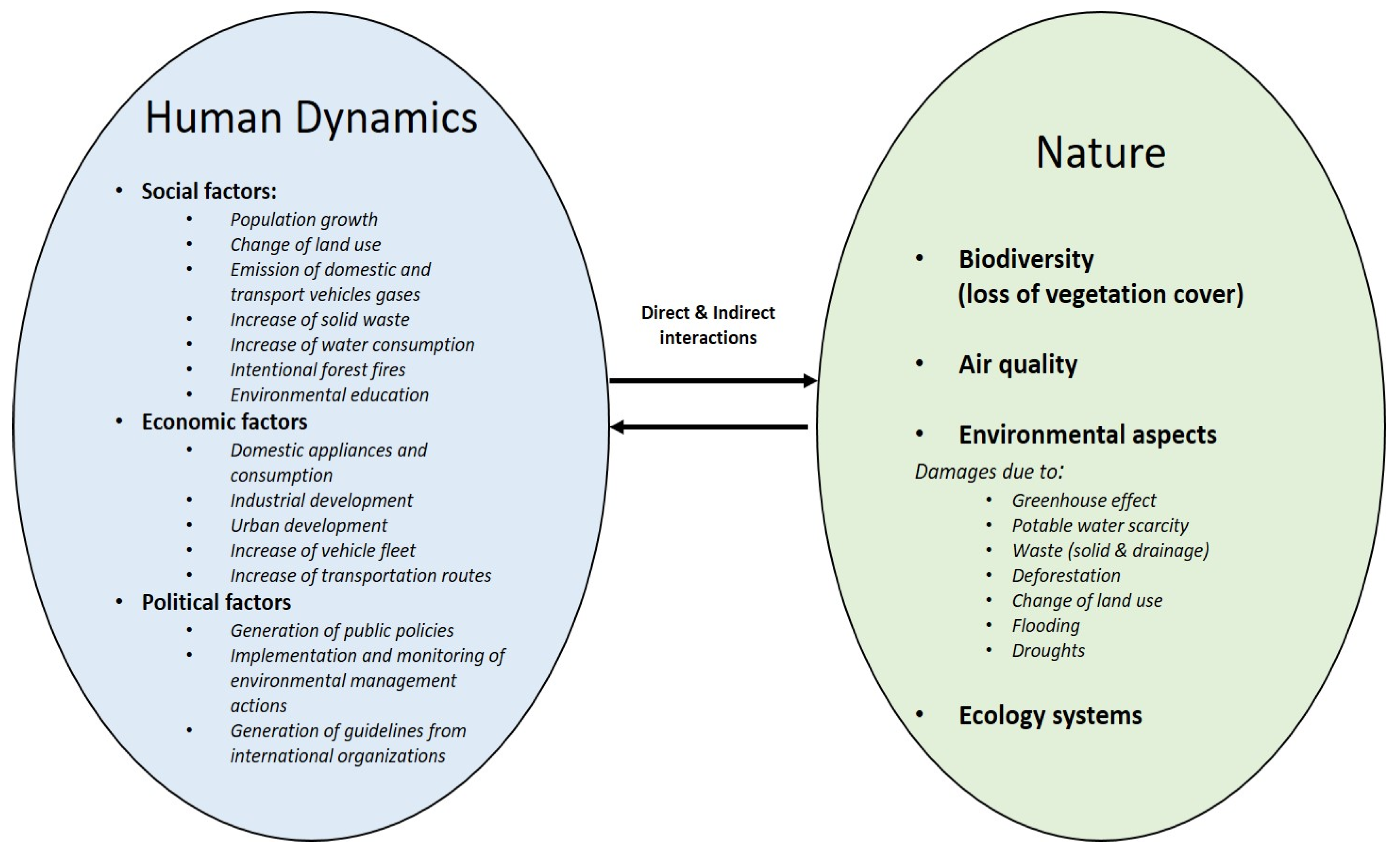
1.1. The Problem of Modeling Multiple Human-Nature Interactions
1.2. The Population Increase and Its Effects on Key Environmental Variables
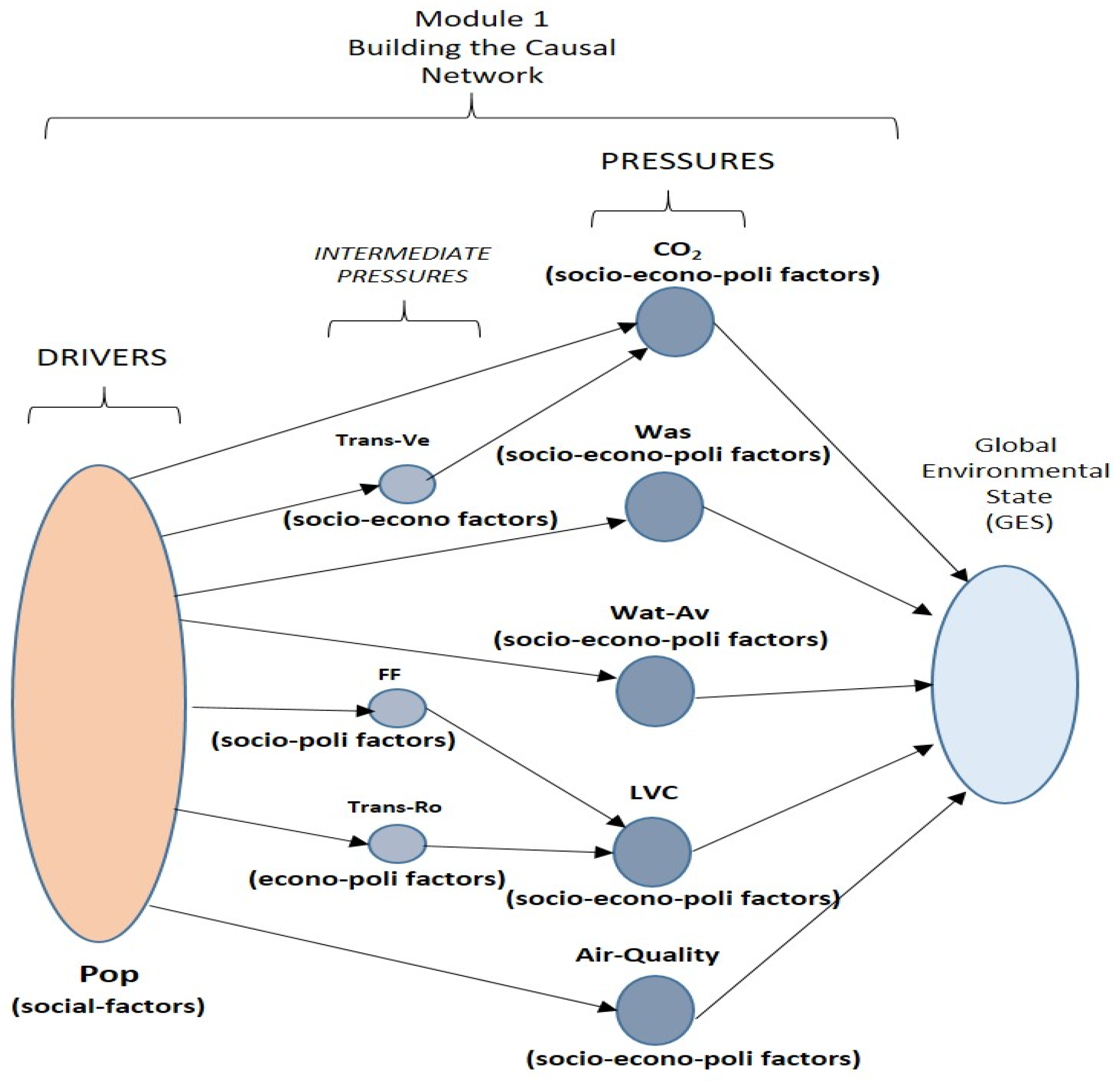
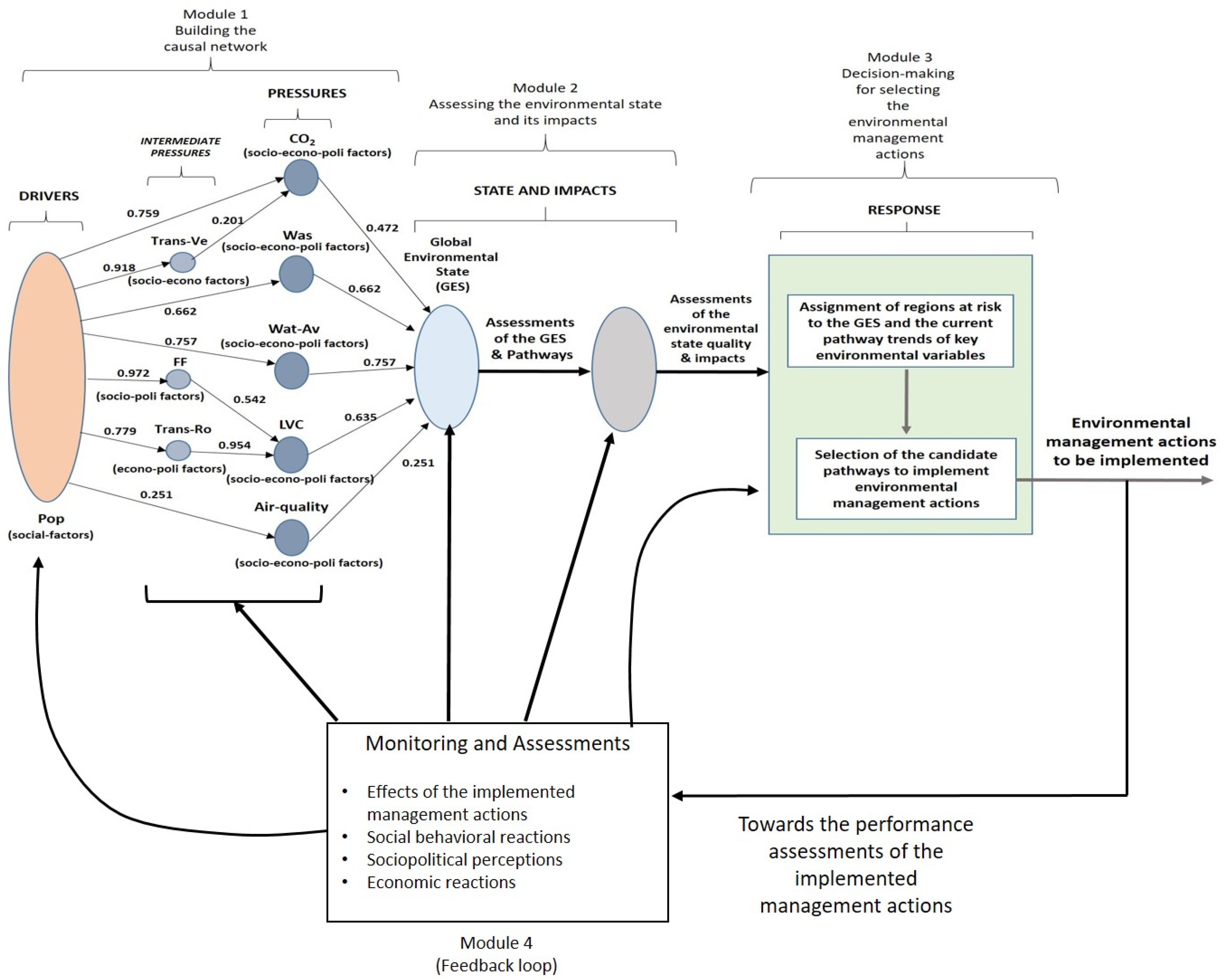
1.3. Conceptual Framework to Build Cause-Effect Relationships between Variables
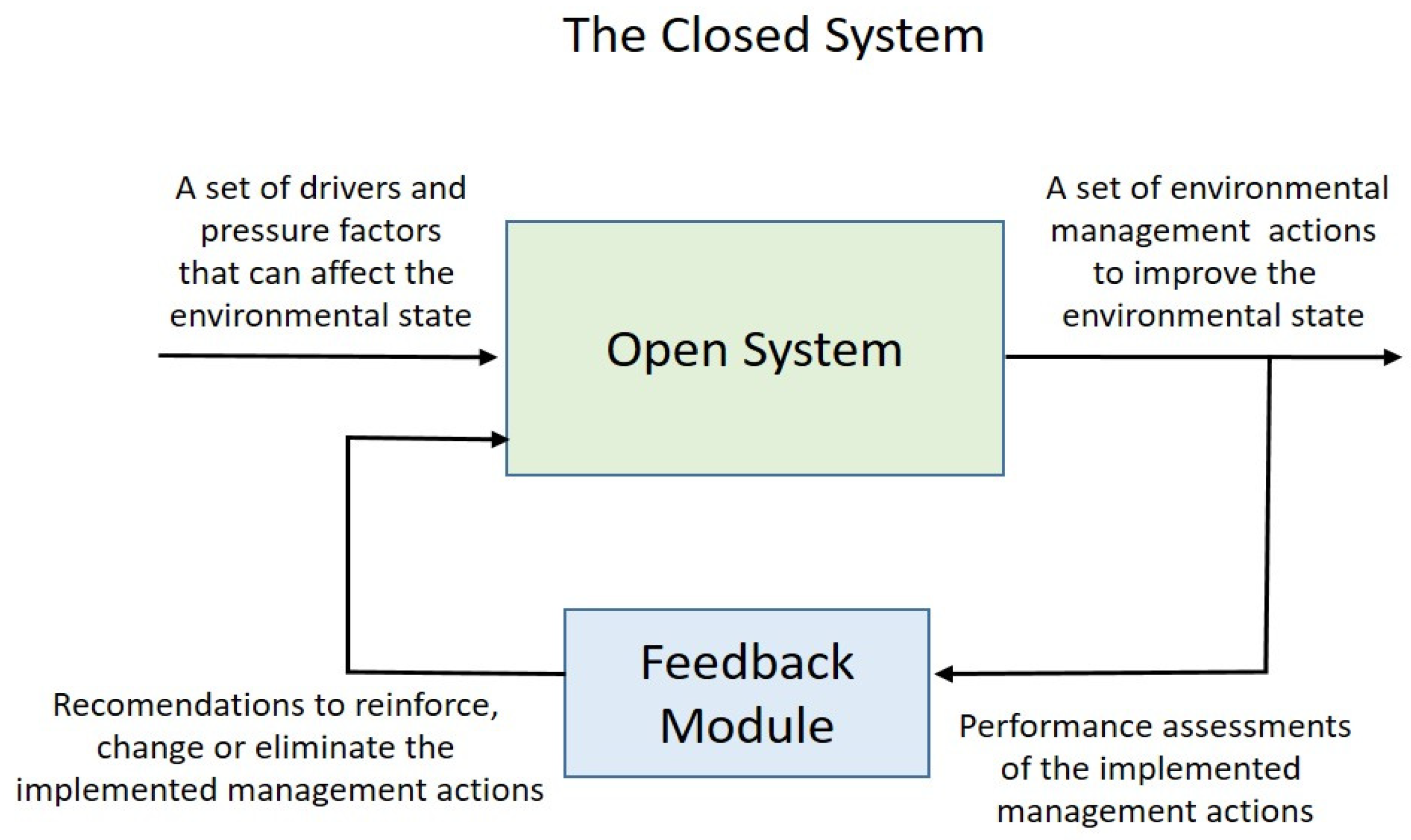
1.4. The Systems Thinking Approach as Support to Build Multiple Interactions
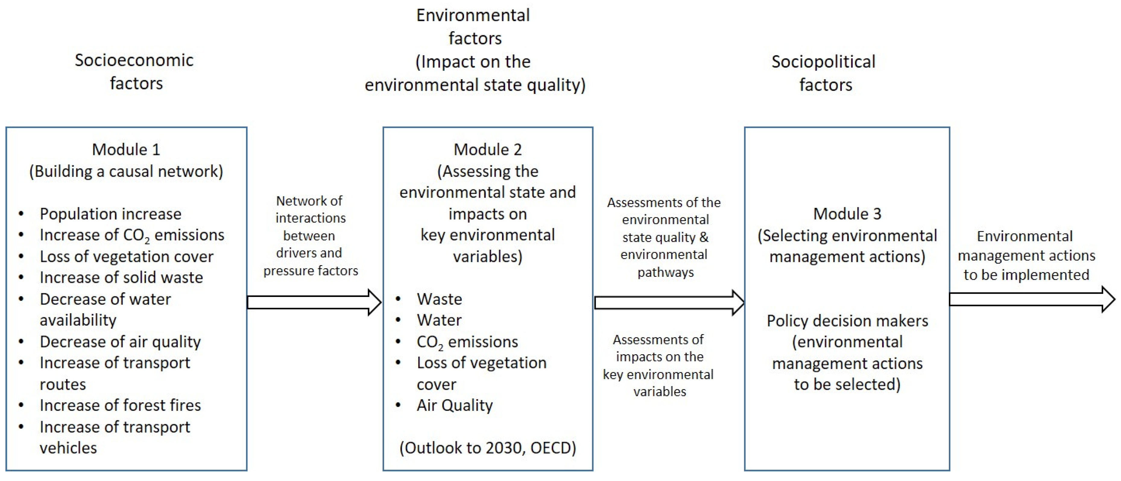
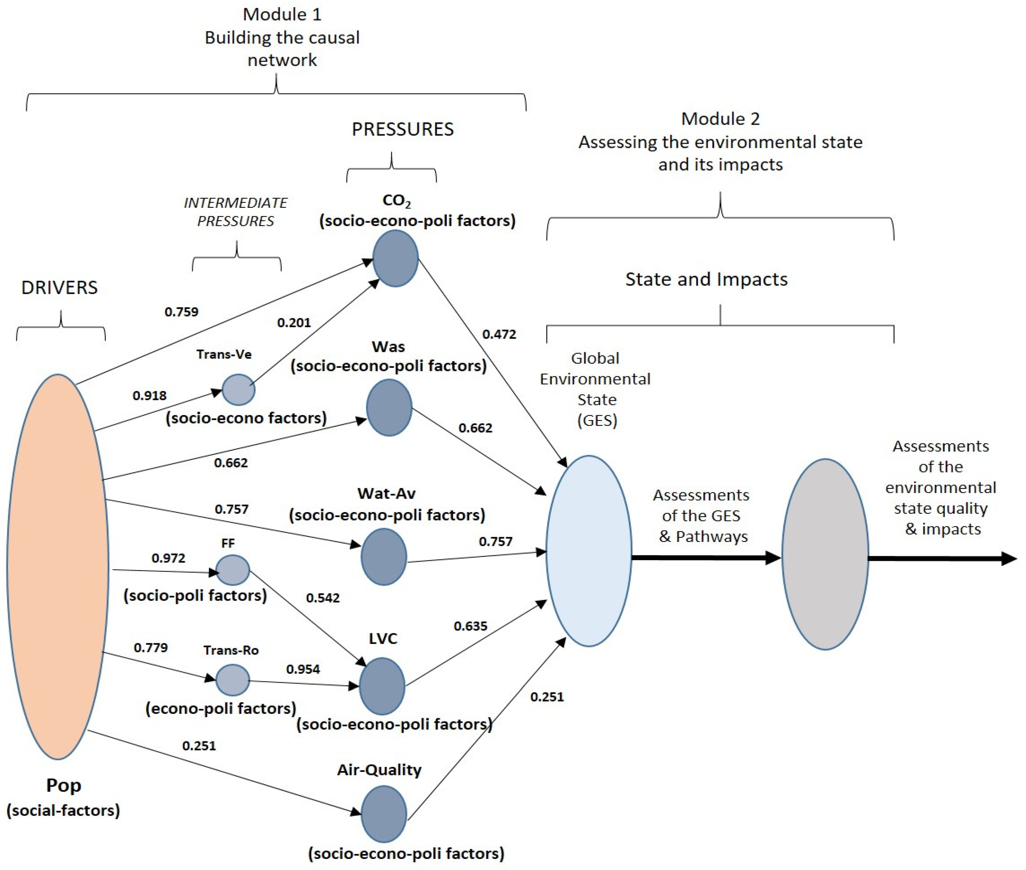
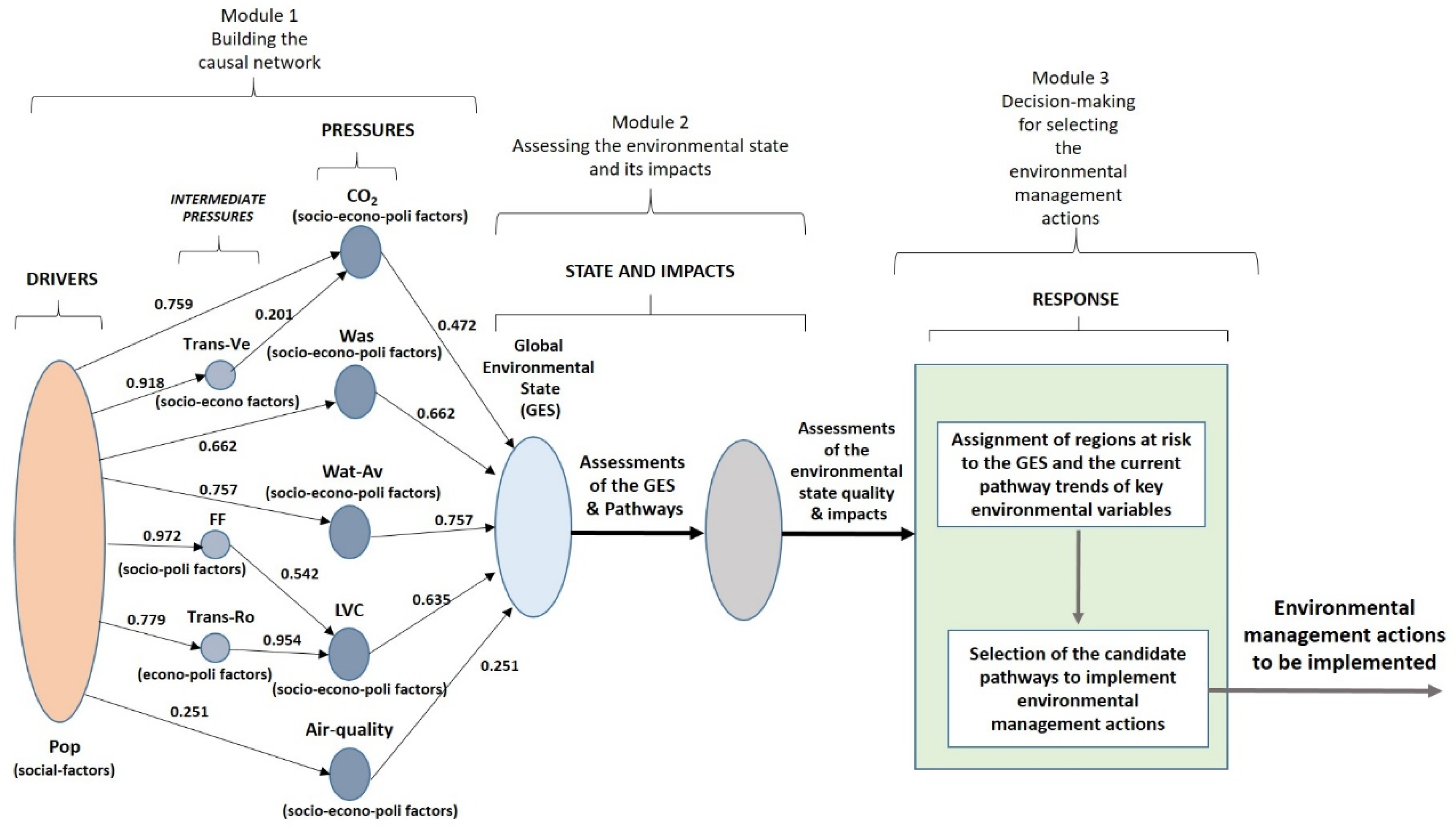
1.5. The Proposal Based on a Systems Thinking Approach
2. Materials and Methods
2.1. Materials
2.2. Methods
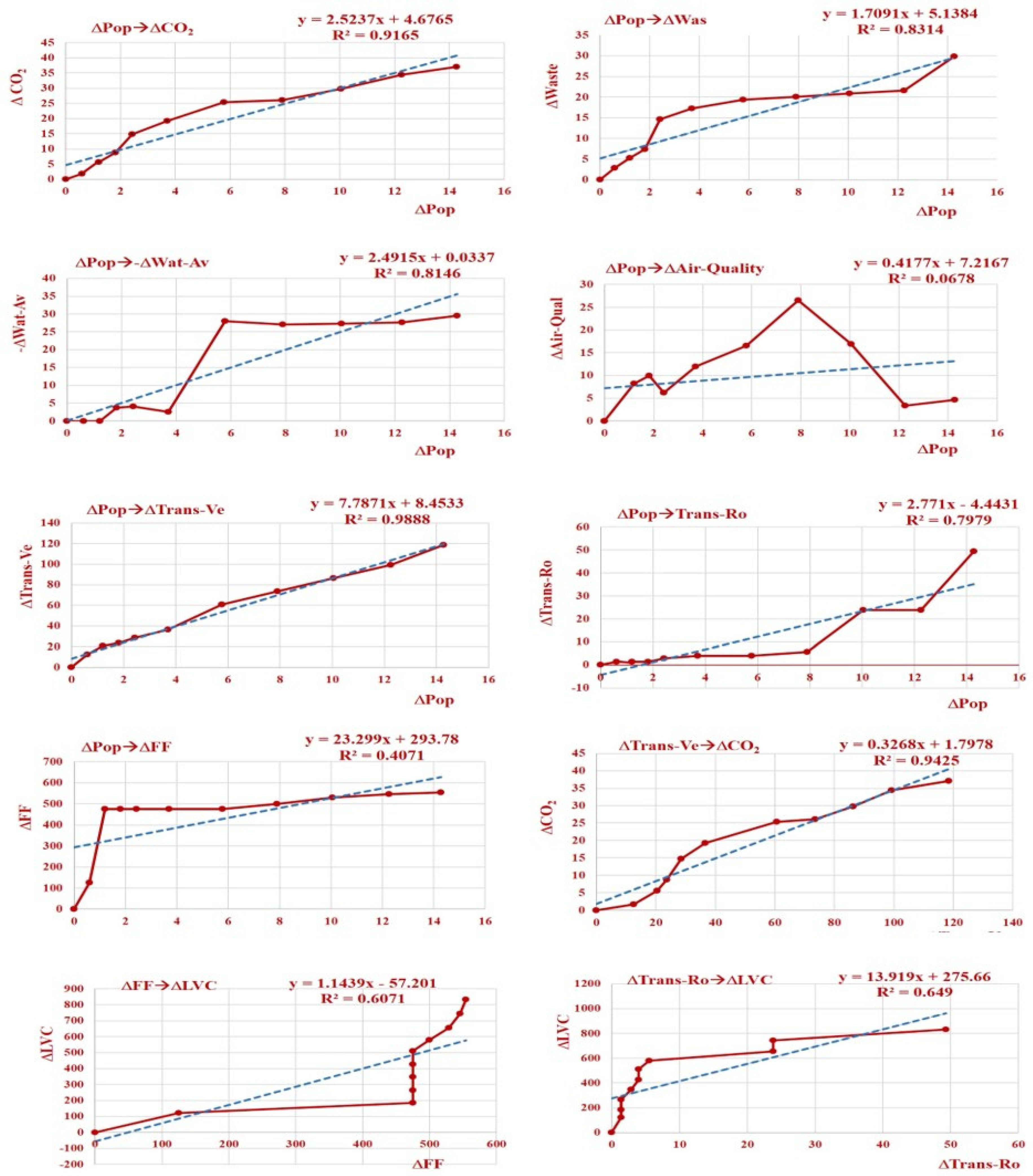
- (ΔPop → ΔFF) ∧ (ΔFF → ΔLVC).
- (ΔPop → ΔTrans-Ro) ∧ (ΔTrans-Ro → ΔLVC)
3. Discussion of Results
4. Conclusions
Author Contributions
Funding
Acknowledgments
Conflicts of Interest
References
- Liu, J.; Dietz, T.; Carpenter, S.R.; Alberti, M.; Folke, C.; Moran, E.; Pell, A.N.; Deadman, P.; Kratz, T.; Lubchenco, J.; et al. Complexity of Coupled Human and Natural Systems. Science 2007, 317, 1513–1516. [Google Scholar] [CrossRef] [PubMed] [Green Version]
- Ratter, B.M.V. Complexity and Emergence—Key concepts in non-linear dynamic systems. In Human-Nature Interactions in Anthropocene; Potentials of Social-Ecological Systems Analysis, Glaser, M., Krause, G., Ratter, B.M.-W., Welp, M., Eds.; Routledge, Taylor and Francies Group: New York, NY, USA, 2012; Chapter 3. [Google Scholar]
- Soga, M.; Gaston, K.J. Extinction of experience: The loss of human–nature interactions. Front. Ecol. Environ. 2016, 14, 94–101. [Google Scholar] [CrossRef]
- Pyle, R.M. The Thunder Tree: Lessons from an Urban Wildland; Houghton Mifflin: Boston, MA, USA, 1993. [Google Scholar]
- Verburg, P.H. Simulating feedbacks in land use and land cover change models. Landsc. Ecol. 2006, 21, 1171–1183. [Google Scholar] [CrossRef]
- Kellert, S.R. Building for Life. Designing and Understanding the Human-Nature Connection; Island Press: Washington, DC, USA, 2005. [Google Scholar]
- OECD. Environmental Outlook to 2030. 2008. Available online: http://www.oecd.org/env/indicators-modelling-outlooks/40200582.pdf (accessed on 15 January 2017).
- Breitburg, D.L.; Baxter, J.W.; Hatfield, C.A.; Howarth, R.W.; Jones, C.G.; Lovett, G.M.; Wigand, C. Understanding effects of multiple stressors: Ideas and challenges. In Successes, Limitation, and Frontiers in Ecosystem Science; Springer: New York, NY, USA, 1998; pp. 416–431. [Google Scholar] [CrossRef]
- McDonald, R.I.; Green, P.; Balk, D.; Fekete, B.M.; Revenga, C.; Todd, M.; Montgomery, M. Urban growth, climate change, and freshwater availability. Proc. Natl. Acad. Sci. USA 2011, 108, 6312–6317. [Google Scholar] [CrossRef] [Green Version]
- Falkenmark, M.; Widstrand, C. Population and water resources: A delicate balance. Popul. Bull. 1992, 47, 1–36. [Google Scholar] [PubMed]
- Carter, R.C.; Parker, A. Climate change, population trends and groundwater in Africa. Hydrol. Sci. J. 2009, 54, 676–689. [Google Scholar] [CrossRef] [Green Version]
- Vörösmarty, C.J.; Green, P.; Salisbury, J.; Lammers, R.B. Global Water Resources: Vulnerability from Climate Change and population growth. Science 2000, 289, 284–288. [Google Scholar] [CrossRef]
- Dyson, B.; Chang, N. Forecasting municipal solid waste generation in a fast-growing urban region with system dynamics modeling. Waste Manag. 2005, 25, 669–679. [Google Scholar] [CrossRef] [PubMed]
- Hoornweg, D.; Bhada-Tata, P.; Kennedy, C. Waste production must peak this century. Nature 2013, 502, 615–617. [Google Scholar] [CrossRef] [PubMed]
- The World Bank. Solid Waste Management. The World Bank. Available online: http://www.worldbank.org/en/topic/urbandevelopment/brief/solid-waste-management (accessed on 20 September 2018).
- Senzige, J.P.; Makinde, O.D. Modelling the Effects of Population Dynamics on Solid Waste Generation and Treatment. Sci. J. Appl. Math. Stat. 2015, 4, 141–146. [Google Scholar] [CrossRef]
- Manaf, L.A.; Samah, M.A.A.; Zukki, N.I.M. Municipal solid waste management in Malaysia: Practices and challenges. Waste Manag. 2009, 29, 2902–2906. [Google Scholar] [CrossRef]
- Minghua, Z.; Xiumin, F.; Rovetta, A.; Qichang, H.; Vicentini, F.; Bingkai, L.; Giusti, A.; Yi, L. Municipal solid waste management in Pudong new area, China. Waste Manag. 2009, 29, 1227–1233. [Google Scholar] [CrossRef] [PubMed]
- Feng, Y.Y.; Chen, S.Q.; Zhang, L.X. System dynamics modeling for urban energy consumption and CO2 emissions: A case study of Beijing, China. Ecol. Model. 2013, 252, 44–52. [Google Scholar] [CrossRef]
- Knapp, T.; Mookerjee, R. Population growth and global CO2 emissions: A secular perspective. Energy Policy 1996, 24, 31–37. [Google Scholar] [CrossRef]
- O’neill, B.C.; Dalton, M.; Fuchs, R.; Jiang, L.; Pachauri, S.; Zigova, K. Global demographic trends and future carbon emissions. Proc. Natl. Acad. Sci. USA 2010, 107, 17521–17526. [Google Scholar] [CrossRef] [PubMed] [Green Version]
- Shi, A. Population growth and global carbon dioxide emissions. In Proceedings of the IUSSP General Conference, Salvador de Bahia, Brazil, 18–24 August 2001. [Google Scholar]
- Guan, D.; Hubacek, K.; Weber, C.L.; Peters, G.P.; Reiner, D.M. The drivers of Chinese CO2 emissions from 1980 to 2030. Glob. Environ. Chang. 2008, 18, 626–634. [Google Scholar] [CrossRef]
- Liang, Y.; Niu, D.; Wang, H.; Li, Y. Factors Affecting Transportation Sector CO2 Emissions Growth in China: An LMDI Decomposition Analysis. Sustainability 2017, 9, 1730. [Google Scholar] [CrossRef]
- Timilsina, G.R.; Shrestha, A. Transport sector CO2 emissions growth in Asia: Underlying factors and policy options. Energy Policy 2009, 37, 4523–4539. [Google Scholar] [CrossRef]
- Syphard, A.D.; Radeloff, V.C.; Keeley, J.E.; Hawbaker, T.J.; Clayton, M.K.; Stewart, S.I.; Hammer, R.B. Human Influence on California Fire Regimes. Ecol. Appl. 2007, 17, 1388–1402. [Google Scholar] [CrossRef] [PubMed]
- Guyette, R.P.; Muzika, R.M.; Dey, D.C. Dynamics of an anthropogenic fire regime. Ecosystems 2002, 5, 472–486. [Google Scholar]
- Contreras-MacBeath, T.; Ongay-Delhumeau, E.; Sorani, D.V. Programa Estatal de Ordenamiento Territorial Sustentable de Morelos. Fases I,I y III; Secretaría de Desarrollo Sustentable: Estado de Morelos, México, 2002. [Google Scholar]
- Trombulak, S.C.; Frisell, C.A. Review of Ecological Effects of Roads on Terrestrial and Aquatic Communities. Conserv. Boil. 2000, 14, 18–30. [Google Scholar] [CrossRef] [Green Version]
- Harte, J. Human population as a dynamic factor in environmental degradation. Popul. Environ. 2007, 28, 223–236. [Google Scholar] [CrossRef]
- OECD. Environmental Indicators: Towards Sustainable Development; Published by the Organization for Economic Cooperation and Development; OECD iLibrary: Paris, France, 2001. [Google Scholar]
- OECD. OECD Environmental Indicators, Development, Measurement and Use. 2003. Available online: https://www.oecd.org/env/indicators-modelling-outlooks/24993546.pdf (accessed on 15 January 2017).
- Omann, I.; Stocker, A.; Jäger, J. Climate change as a threat to biodiversity: An application of the DPSIR approach. Ecol. Econ. 2009, 69, 24–31. [Google Scholar] [CrossRef]
- Mysiak, J.; Giupponi, C.; Rosato, P. Towards the development of a decision support system for water resource management. Environ. Model. Softw. 2005, 20, 203–214. [Google Scholar] [CrossRef]
- Lynch, A.J.J. The usefulness of a threat and disturbance categorization developed for Queensland wetlands to environmental management, monitoring and evaluation. Environ. Manag. 2011, 47, 40–55. [Google Scholar] [CrossRef]
- Keible, C.R.; Loomis, D.K.; Lovelace, S.; Nuttle, W.K.; Ortner, P.B.; Fletcher, P.; Cook, G.S.; Lorenz, J.J.; Boyer, J.N. The EBM-DPSER conceptual model: Integrating ecosystem services into the DPSIR framework. PLoS ONE 2013, 8, e70766. [Google Scholar]
- Gari, S.R.; Newton, A.; Icely, J.D. A review of the application and evolution of the DPSIR framework with an emphasis on coastal social-ecological systems. Ocean Coast. Manag. 2005, 103, 63–77. [Google Scholar] [CrossRef]
- Nezami, S.R.; Nazariha, M.; Moridi, A.; Baghvand, A. Environmentally sound water resources management in catchment level using DPSIR model and scenario analysis. Int. J. Environ. Res. 2013, 7, 569–580. [Google Scholar]
- Anupam, K. Application of the DPSIR Framework for Municipal Solid Waste Management in South Asian Developing Countries. PhD. Thesis, Graduate School of Engineering, Osaka University, Osaka, Japan, 2010. [Google Scholar]
- Nikolaou, K.; Basbas, S.; Taxiltaris, C. Assessment of air pollution indicators in an urban area using the DPSIR model. Fresenius Environ. Bull. 2004, 13, 820–830. [Google Scholar]
- Wang, W.; Yuhong, Y.; Wu, J. Environmental Warning System Based on the DPSIR Model: A Practical and Concise Method for Environmental Assessment. Sustainability 2018, 10, 1728. [Google Scholar] [CrossRef]
- Senge, P. The Fifth Discipline; Doubleday: New York, NY, USA, 1990. [Google Scholar]
- Dominici, G. Why Does Systems Thinking Matter? Bus. Syst. Rev. 2012, 1, 1–2. [Google Scholar] [CrossRef]
- Arnold, R.D.; Wade, J.P. A Definition of Systems Thinking: A Systems Approach. Procedia Comput. Sci. 2015, 44, 669–678. [Google Scholar] [CrossRef] [Green Version]
- Richmond, B. System dynamics/systems thinking: Let’s just get on with it. In International Systems Dynamics Conference, Sterling, Scotland; Wiley Online Library: Hoboken, NJ, USA, 1994. [Google Scholar]
- Meadows, D.H. Thinking in Systems: A Primer; Chelsea Green Publishing: White River Junction, VT, USA, 2008. [Google Scholar]
- Sweeney, L.B.; Sterman, J.D. Bathtub dynamics: Initial results of a systems thinking inventory. Syst. Dyn. Rev. 2000, 16, 249–286. [Google Scholar] [CrossRef]
- Forrester, J.W. System dynamics, systems thinking, and soft OR. Syst. Dyn. Rev. 1994, 10, 245–256. [Google Scholar] [CrossRef]
- Behl, D.V.; Ferreira, S. Systems Thinking: An Analysis of Key Factors and Relationships. Procedia Comput. Sci. 2014, 36, 104–109. [Google Scholar] [CrossRef] [Green Version]
- Davidz, H.L.; Nightingale, D.J. Enabling Systems Thinking to Accelerate the Development of Senior Systems Engineers. Syst. Eng. 2008, 11, 1–14. [Google Scholar] [CrossRef]
- Moore, S.M.; Dolansky, M.A.; Singh, M.; Palmieri, P.; Alemi, F. The Systems Thinking Scale; Case Western Reserve University: Cleveland, OH, USA, 2010. [Google Scholar]
- Kasser, J.; Hitchins, D.; Frank, M.; Zhao, Y.Y. A framework for benchmarking competency assessment models. J. Syst. Eng. 2013, 16, 29–44. [Google Scholar] [CrossRef]
- Maani, K.E. Decision-Making for Climate Change Adaptation a Systems Thinking Approach; Synthesis and Integrative Research Final Report NCCARF; University of Queensland: Brisbane, Queensland, Australia, 2013. [Google Scholar]
- Nguyen, N.C.; Bosch, O.J. A systems thinking approach to identify leverage points for sustainability: A case study in the Cat Ba Biosphere Reserve, Vietnam. Syst. Res. Behav. Sci. 2013, 30, 104–115. [Google Scholar] [CrossRef]
- Smith, T. Using critical systems thinking to foster an integrated approach to sustainability: A proposal for development practitioners. Environ. Dev. Sustain. 2011, 13, 1–17. [Google Scholar] [CrossRef]
- Hjorth, P.; Bagheri, A. Navigating towards sustainable development: A system dynamics approach. Futures 2006, 38, 74–92. [Google Scholar] [CrossRef]
- Palmberg, I.; Hofman-Bergholm, M.; Jeronen, E.; Yli-Panula, E. Systems thinking for understanding sustainability? Nordic student teachers’ views on the relationship between species identification, biodiversity and sustainable development. Educ. Sci. 2017, 7, 72. [Google Scholar] [CrossRef]
- Onat, N.; Kucukvar, M.; Halog, A.; Cloutier, S. Systems thinking for life cycle sustainability assessment: A review of recent developments, applications, and future perspectives. Sustainability 2017, 9, 706. [Google Scholar] [CrossRef]
- INEGI. Instituto Nacional de Estadística y Geografía. Perspectiva Estadística; INEGI: Aguascalientes, México, 2011. [Google Scholar]
- INEGI. Instituto Nacional de Estadística y Geografía. 2016. Available online: http://www3.inegi.org.mx (accessed on 15 January 2017).
- SCT. Secretaría de Comunicaciones y Transportes. Anuario Estadístico 2011, México. 2012. Available online: http://www.sct.gob.mx/planeacion/estadistica/anuario-estadistico-sct/ (accessed on 15 January 2017).
- SEMARNAT. Secretaría de Medio Ambiente y Recursos Naturales, Comisión Nacional Forestal, Gerencia de Incendios Forestales (SEMARNAT). 2012. Available online: http://www.conafor.gob.mx/web/temas-forestales/ (accessed on 15 January 2017).
- GFW. Global Forest Watch. 2014. Available online: http://www.globalforestwatch.org (accessed on 15 January 2017).
- Secretaría de Medio Ambiente y Recursos Naturales-Comisión Nacional del Agua (SEMARNAT-CONAGUA). Programa Hídrico Visión 2030 del Estado de Morelos; Secretariat of Environment and Natural Resources (SEMARNAT): Cuernavaca, México, 2010. [Google Scholar]
- SNIARNF-SEMARNAT. Sistema Nacional de Información Ambiental y de Recursos Naturales (Módulo de Consulta Temática, Dimensión Ambiental, Generación de Residuos Sólidos Urbanos. 2012. Available online: http://dgeiawf.semarnat.gob.mx (accessed on 15 January 2017).
- UNFCCC. United Nations Framework Convention on Climate Change. 2014. Available online: http://unfccc.int/national_reports/nonannex_i_natcom/training_material/methodological_documents/items/349.php (accessed on 15 January 2017).
- Draxler, R.R.; Rolph, G.D. HYSPLIT—Hybrid Single-Particle Lagrangian Integrated Trajectory Model. Available online: http://www.arl.noaa.gov/HYSPLIT.php (accessed on 22 October 2018).
- Sims, K.R.; Alix-García, J.M.; Shapiro-Garza, E.; Fine, L.R.; Radeloff, V.C.; Aronson, G.; Castillo, S.; Ramírez-Reyes, C.; Yañez-Pagans, P. Improving environmental and social targeting through adaptive management in Mexico’spayments for hydrological services program. Conserv. Biol. 2014, 28, 1151–1159. [Google Scholar] [CrossRef] [PubMed]
- González, M.; Aldrete, A.; Gómez, A.; López, C.; de los Santos, H.; Benavides, J.; Vargas, J.; Valdez, J.; Hernández, P.; Fernández, S. Estudio de Mercado del Servicio Ambiental Hidrológico en la Cuenca de Tapalpa, Jalisco. Estudio de Caso; Anexo 33. Evaluación del Programa de Pago por Servicios Ambientales de la Comisión Nacional Forestal; Gobierno del estado de Jalisco: Tepalpa, México, 2005. [Google Scholar]


| Relationships | Observations and Statistical Data |
|---|---|
| Population increase causes water availability to decrease. | In 2000, 150 million people lived in cities with perennial water shortage (i.e., annual water availability <100 L/person/day) within their urban extent. Based on a forecast, in 2050, 993 million of people will live in cities with perennial water shortage within their urban extent [9]. Other related work is found in [10,11,12]. |
| Population increase causes increase in solid waste. | Based on a study of the population increase versus the increase of generation of solid waste in San Antonio Texas, USA: 1980: population = 786,023; solid waste = 154,983 (tons) 2010: population = 1,323,956; solid waste = 366,125 (tons) Conclusion: the population increased 168.43 % in 2010 with respect to 1980; whereas, the solid waste generation increased 236.23% in 2010 with respect to 1980. Thus, the percentage increase of solid waste generation increased was bigger than the percentage increase of population [13]. Urban waste production has risen tenfold compared with the growth of urban population [14]. Other related work is found in [15,16,17,18]. |
| Population increase brings about increases in CO2 emissions. | A model for Beijing, China shows that the intensified urban development and the expanded population demand more energy consumption, thus increasing the CO2 emissions. The CO2 emissions will increase from 118.41 MtCO2 in 2005 to 169 MtCO2 in 2030 [19]. Other related work [20,21,22,23]. |
| Population increase results in increase in the transportation sector, which in turn causes CO2 emissions to increase. | Population size increased 7.92%: from 1267.43 × 106 in the year 2000 to 1367.82 × 104 in 2014. GDP increased 272.50%: from 1,311,691 × 106 (euros) in the year 2000 to 4,886,144 × 106 (euros) in the year 2014. CO2 emissions of the transportation sector increased 218.23%: from 32,584.03 × 104 (tons) in 2000 to 103,695.38 × 104 (tons) in 2014. The combination of population increase with the economic power increase brought about an increase of 218.23% in CO2 emissions from 2000 to 2014 [24]. One more related work: [25]. |
| Population growth influences fires, thus causing losses of vegetation cover. | This research uses two concepts of wildland-urban interfaces (WUI) to study the human influence on the fire regimes of California: the interface WUI, where development abuts wildland vegetation, and the intermix WUI, where development intermingles with wildland vegetation. Based on nonlinear anthropogenic relationships the following thresholds were estimated suggesting that fire frequency is likely to be highest when population density is between 35 and 45 people/Km2, the proportion of intermix WUI is ~20–30%; the proportion of intermix WUI is ~25–35%, the mean distance to intermix WUI is <9 km, and the mean distance to interface WUI is <14 km. The majority of fires are burning closer to developed areas, whose human presence is normal. Therefore, future conditions that include continued growth of intermix WUI may also contribute to greater fire risk and devastating ecological impacts may take place if development continues to grow farther into wildland [26]. Other related work [27,28]. |
| Year | Pop (Persons) (Driver-Var) | CO2 (Gg) (Press-Var) | Trans-Ro (Km) (Press-Var) | FF (Ha) (Press-Var) | LVC (Ha) (Press-Var) | Wat-Av (m3/per) (Press-Var) | Trans-Ve (Num. Vehicles) (Press-Var) | Was (Tons) (Press-Var) | Air-Quality (PM2.5) (mass/m3) (Press-Var) |
|---|---|---|---|---|---|---|---|---|---|
| 2000 | 1,555,296 | 2816.2 | 2001 | 12 | 90.4 | 2.818 | 155,600 | 459,000 | 1.01603 × 10⁻⁸ |
| 2001 | 1,564,627 | 2865.27 | 2029 | 27 | 201.5 | 2.818 | 175,000 | 472,000 | No-Data |
| 2002 | 1,574.015 | 2974.88 | 2029 | 69 | 257.0 | 2.818 | 187,500 | 483,000 | 1.00925 × 10⁻⁸ |
| 2003 | 1,583,459 | 3064.54 | 2029 | 69 | 329.7 | 2.713 | 192,500 | 493,000 | 1.11715 × 10⁻⁸ |
| 2004 | 1,592,960 | 3231.57 | 2058 | 69 | 405.3 | 2.701 | 200,000 | 526,000 | 1.07855 × 10⁻⁸ |
| 2005 | 1,612,899 | 3358.76 | 2080 | 69 | 476.1 | 2.746 | 212,500 | 538,000 | 1.13786 × 10⁻⁸ |
| 2006 | 1,645,157 | 3530.68 | 2080 | 69 | 551.3 | 2.029 | 250,000 | 548,000 | 1.18449 × 10⁻⁸ |
| 2007 | 1,678,060 | 4552.01 | 2112 | 72 | 613.7 | 2.055 | 270,000 | 551,000 | 1.28523 × 10⁻⁸ |
| 2008 | 1,711,621 | 3652.88 | 2477 | 75.5 | 681.8 | 2.049 | 290,000 | 555,000 | 1.18733 × 10⁻⁸ |
| 2009 | 1,745,854 | 3784.18 | 2477 | 77.5 | 762.7 | 2.040 | 310,000 | 558,000 | 1.04967 × 10⁻⁸ |
| 2010 | 1,777,227 | 3859.22 | 2986 | 78.5 | 843.3 | 1.987 | 340,000 | 596,000 | 1.06340 × 10⁻⁸ |
| Key Environmental Variables | Environmental Management Actions |
|---|---|
| Waste |
|
| Water |
|
| Air-Quality |
|
| CO2 Emissions |
|
| Loss of Vegetation Cover |
|
| Causal Relationships | Type of Relationship | Observations/Interpretations |
|---|---|---|
| ΔPop → ΔWas | Direct | If population increases, then waste generation increases |
| ΔPop → -ΔWat-Av | Direct | If population increases, then water availability decreases |
| ΔPop → ΔAir-Quality | Direct | If population increases, then the air-quality decreases |
| ΔPop → ΔTrans-Ro | Direct | If population increases, then transportation roads increase |
| ΔPop → ΔFF | Direct | If population increases, then forest fires increase |
| ΔPop → ΔTrans-Ve | Direct | If population increases, then the number of vehicles increases |
| ΔPop → ΔCO2 | Direct | If population increases, then household appliances increase, which contributes to increase CO2 emissions |
| ΔPop → ΔTrans-Ve → ΔCO2 | Indirect | If population increases, then the number of transport vehicles increases, which will contribute to increase the CO2 emissions |
| ΔPop → ΔFF → ΔLVC | Indirect | If population increases, then forest fires (intentional or no-intentional) increase, thus increasing the loss of vegetation cover. |
| ΔPop → ΔTrans-Ro → ΔLVC | Indirect | If population increases, then the roads of transportation increase, thus increasing the loss of vegetation cover |
| Year | ΔPop (%) | ΔCO2 (%) | ΔTrans-Ro (%) | ΔFF (%) | ΔLVC (%) | ΔWat-Av (%) | ΔTrans-Ve (%) | ΔWas (%) | ΔAir-Quality (%) |
|---|---|---|---|---|---|---|---|---|---|
| 2000 | 0 | 0 | 0 | 0 | 0 | 0 | 0 | 0 | 0 |
| 2001 | 0.600 | 1.742 | 1.399 | 125 | 122.8 | 0 | 12.468 | 2.832 | 0 |
| 2002 | 1.204 | 5.634 | 1.399 | 475 | 184.29 | 0 | 20.501 | 5.229 | 8.191 |
| 2003 | 1.811 | 8.818 | 1.399 | 475 | 264.71 | 3.726 | 23.715 | 7.407 | 9.952 |
| 2004 | 2.422 | 4.749 | 2.848 | 475 | 348.34 | 4.081 | 28.535 | 14.597 | 6.153 |
| 2005 | 3.704 | 19.265 | 3.948 | 475 | 426.65 | 2.555 | 36.568 | 17.211 | 11.99 |
| 2006 | 5.778 | 25.370 | 3.948 | 475 | 509.84 | 27.999 | 60.668 | 19.390 | 16.58 |
| 2007 | 7.893 | 26.127 | 5.547 | 500 | 578.87 | 27.076 | 73.522 | 20.044 | 26.49 |
| 2008 | 10.051 | 29.709 | 23.788 | 529.16 | 654.20 | 27.289 | 86.375 | 20.915 | 16.86 |
| 2009 | 12.252 | 34.371 | 23.788 | 545.83 | 743.69 | 27.608 | 99.229 | 21.569 | 3.311 |
| 2010 | 14.269 | 37.036 | 49.325 | 554.16 | 832.85 | 29.489 | 118.509 | 29.847 | 4.662 |
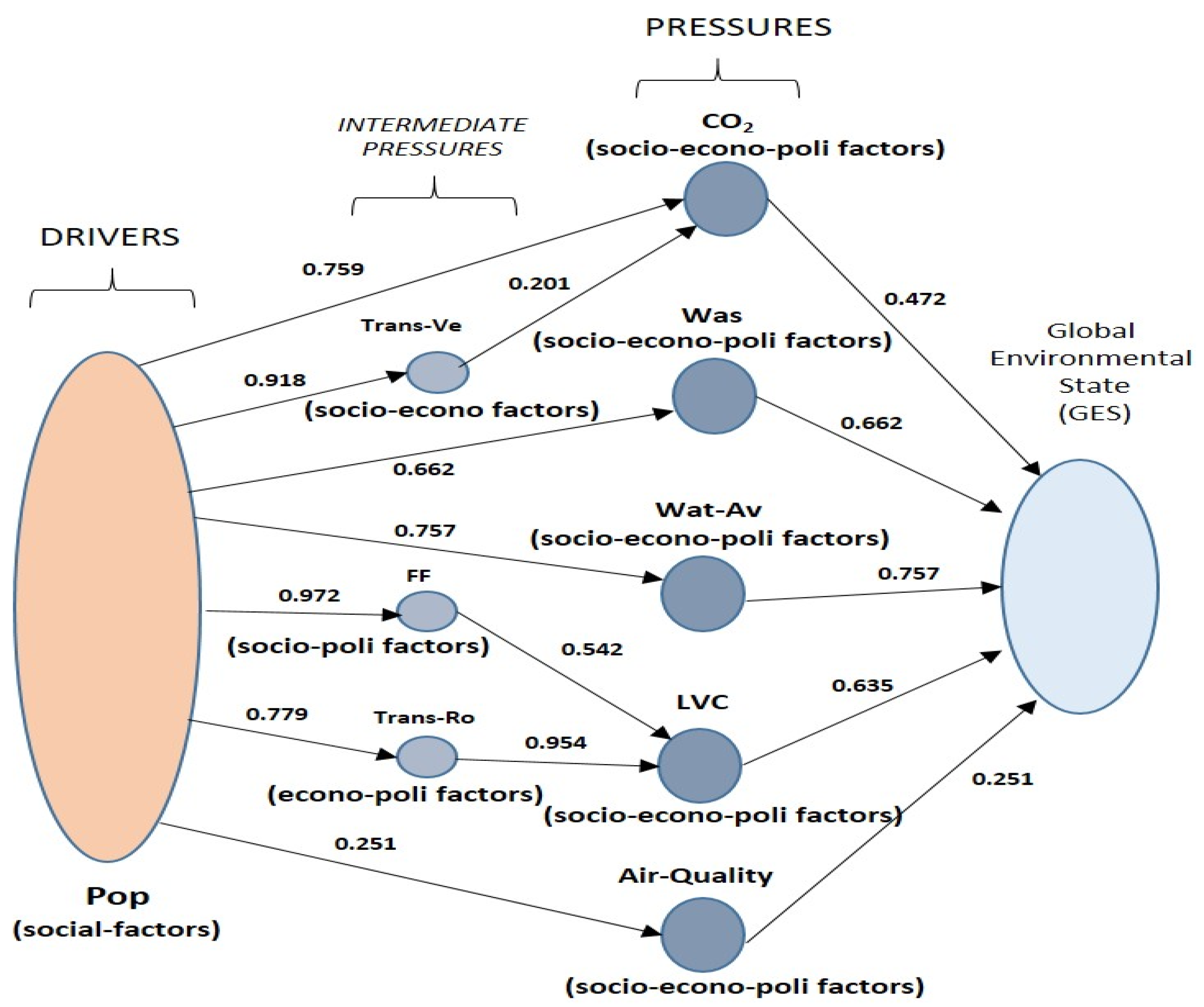
| Causal Relationships | Tangent Value | Angular Value | Normalized Value |
|---|---|---|---|
| ΔPop → ΔCO2 | 2.5237 | 68.38° | 0.759 |
| ΔPop → ΔWas | 1.7091 | 59.66° | 0.662 |
| ΔPop → ΔWat-Av | 2.491 | 68.13° | 0.757 |
| ΔPop → -ΔAir Quality | 0.4177 | 22.67° | 0.251 |
| ΔPop → ΔTrans-Ve | 7.7871 | 82.68° | 0.918 |
| ΔPop → ΔTrans-Ro | 2.7718 | 70.16° | 0.779 |
| ΔPop → ΔFF | 23.299 | 87.54° | 0.972 |
| ΔTrans-Ve → ΔCO2 | 0.3268 | 18.09° | 0.201 |
| ΔFF → ΔLVC | 1.143 | 48.83° | 0.542 |
| ΔTrans-Ro → ΔLVC | 13.919 | 85.89° | 0.954 |
| The Pathways | Tangent Value | Angular Value | Normalized Value |
|---|---|---|---|
| Direct Pathways | |||
| Path_Was = (ΔPop → ΔWas) | 1.709 | 59.67° | 0.662 |
| Path_Wat-Av = (ΔPop → -ΔWat-Av) | 2.491 | 68.13° | 0.757 |
| Path_Air-Quality = ((ΔPop → -∇Air-Quality) | 0.417 | 22.67° | 0.251 |
| Indirect Pathways | |||
| Path_CO2 = (((ΔPop → ΔTrans-Ve)∧(ΔTrans-Ve → ΔCO2)) + (ΔPop → ΔCO2)))/2 | 0.915 | 42.48° | 0.472 |
| Path_LVC = (((ΔPop → ΔFF) ∧ (ΔFF → ΔLVC)) + ((ΔPop → ΔTrans-Ro) ∧ (ΔTrans-Ro → ΔLVC)))/2 | 1.548 | 57.15° | 0.635 |
| The Involved Variables | Year 2000 | Year 2010 | Percentage Difference between the Year 2010 and the Year 2000 |
|---|---|---|---|
| Population (persons) | 1,555,296 | 1,777,227 | 14.269% |
| CO2 emissions (Gg) | 2816.2 | 3859.22 | 37.036% |
| Waste (tons) | 459,000 | 596,000 | 29.847% |
| Loss of water availability (m3/person) | 2818 | 1987 | 29.489% |
| Loss of vegetation cover (ha) | 90.4 | 843.3 | 832.85% |
| Air quality (mass/m3) | 1.01603 × 10⁻⁸ | 1.0634 × 10⁻⁸ | 4.662% |
| Vehicles of transport (number of vehicles) | 155,600 | 340,000 | 118.509% |
| Transport routes (km) | 2001 | 2986 | 49.225% |
| Forest fires (adults trees in hectares) | 12 | 78.5 | 554.16% |
| Regions at Risk | Ranges of the Trends in Angular Values | Ranges of the Trends in Tangent Values |
|---|---|---|
| Very low risk | [0°, 20°) | [0, 36,397) |
| Low risk | [20°, 40°) | [0.36397, 0.83909) |
| Medium risk | [40°, 60°) | [0.83909, 1.73205) |
| High risk | [60°, 80°) | [1.73205, 5.6718) |
| Very high risk | [80°, 90°] | [5.6718, ∞] |
| Year | LVC (ha) | Percentage Increase LVC | NPA (ha) | Percentage Increase NPA |
|---|---|---|---|---|
| 2000 | 90.4 | 0 | 120,020.31 | 0 |
| 2001 | 201.5 | 112.8 | 120,020.31 | 0 |
| 2002 | 257.0 | 184.29 | 120,020.31 | 0 |
| 2003 | 329.7 | 264.71 | 120,020.31 | 0 |
| 2004 | 405.3 | 348.34 | 120,020.31 | 0 |
| 2005 | 476.1 | 426.65 | 120,020.31 | 0 |
| 2006 | 551.3 | 509.84 | 120,020.31 | 0 |
| 2007 | 613.7 | 578.87 | 120,020.31 | 0 |
| 2008 | 681.8 | 654.20 | 128,397.33 | 6.979 |
| 2009 | 762.7 | 743.69 | 128,397.33 | 6.979 |
| 2010 | 843.3 | 832.85 | 128,656.26 | 7.195 |
© 2019 by the authors. Licensee MDPI, Basel, Switzerland. This article is an open access article distributed under the terms and conditions of the Creative Commons Attribution (CC BY) license (http://creativecommons.org/licenses/by/4.0/).
Share and Cite
Ramos-Quintana, F.; Sotelo-Nava, H.; Saldarriaga-Noreña, H.; Tovar-Sánchez, E. Assessing the Environmental Quality Resulting from Damages to Human-Nature Interactions Caused by Population Increase: A Systems Thinking Approach. Sustainability 2019, 11, 1957. https://doi.org/10.3390/su11071957
Ramos-Quintana F, Sotelo-Nava H, Saldarriaga-Noreña H, Tovar-Sánchez E. Assessing the Environmental Quality Resulting from Damages to Human-Nature Interactions Caused by Population Increase: A Systems Thinking Approach. Sustainability. 2019; 11(7):1957. https://doi.org/10.3390/su11071957
Chicago/Turabian StyleRamos-Quintana, Fernando, Héctor Sotelo-Nava, Hugo Saldarriaga-Noreña, and Efraín Tovar-Sánchez. 2019. "Assessing the Environmental Quality Resulting from Damages to Human-Nature Interactions Caused by Population Increase: A Systems Thinking Approach" Sustainability 11, no. 7: 1957. https://doi.org/10.3390/su11071957