Agent-Based Modeling of Sustainable Ecological Consumption for Grasslands: A Case Study of Inner Mongolia, China

Abstract

Sustainable ecosystem services consumption is of vital importance to the survival and development of human society. How to balance the conflicts between ecosystem protection and ecosystem services consumption by local residents has been a serious challenge, especially in ecologically vulnerable areas. To explore the reasonable ecosystem services consumption approaches of grassland ecosystems for sustainable land system management, this study takes Hulun Buir of the Inner Mongolia Autonomous Region as a case study region and develops an EcoC-G (ecological consumption of grassland) model based on herders’ livelihood behaviors using the agent-based model technique to simulate the dynamics of ecosystem pressure, livestock production, and living quality of herders under different grassland management scenarios over the next 30 years. The EcoC-G model links the supply and consumption of grassland ecosystem services by calculating the ecosystem net primary productivity (NPP) supply and household NPP consumption. The model includes three sub-models, namely, the individual status transferring sub-model, the households’ grassland-use decision sub-model, and the ecosystem pressure sub-model. In accordance with multi-objective grassland management practices, the following four land management scenarios were simulated: (1) baseline scenario, (2) increasing household’s living standard, (3) ecosystem protection, and (4) balancing living standard improvement with the protection of the ecosystem. The result indicates that by focusing on the NPP supply and consumption of the grassland ecosystem, the EcoC-G is capable of simulating the impacts of herders’ livelihood behaviors on grassland ecosystems. If timely grassland management strategies are implemented, it is possible to relieve the ecosystem pressure and improve the livelihood of local herders. The specific scenario simulation results are: (1) Under the current grassland management mode, the pasture could never be overgrazed, and herders could achieve the basic living standard, but the accumulated wealth decreased due to the decline of livestock. (2) With grazing control, herders can accumulate wealth by increasing the breeding amount and reducing the marketing rate, but the ecosystem consumption pressure can reach a maximum of 2.3 times. (3) With strict restrictions on the livestock number, the pressure on the ecosystem decreases; however, herders might not achieve basic living standards. (4) Modest regulation leads to rational ecological consumption intervals, meaning the ecosystem pressure will become stable and herders can gradually accumulate wealth with the achievement of basic living standards in advance.

1. Introduction

The increasing demand by human beings for food, energy, fibers, and other materials has stimulated the consumption of limited natural resources from the Earth’s surface [1,2]. The excessive usage of natural resources has further intensified the contradictions between the maintenance of ecosystem service function and economic growth [3]. The Food and Agriculture Organization (Roman, Italy) of the United Nations in 2011 indicated that up to 25% of all land worldwide is highly degraded, and 36% is slightly or moderately degraded [4]. This condition threatens sustainable land management at the local, regional, and global levels [5]. How to balance ecosystem safety and human well-being for social–ecological system sustainability has become a critical issue that fully concerns the scientific community and policy makers [6].

In Inner Mongolia, which is a vulnerable ecological region in China, the problems mentioned above also exist [7,8]. Over the past 30 years, pasture has been utilized intensively, with continuous overgrazing in the area to meet the requirements of the increasing population and the changing lifestyle from a traditional nomadic style to a modern settled-down style [9], which has resulted in unprecedented overgrazing and tremendous land degradation [10]. From 1985 to 1999, the degraded steppe in the Xilin River Basin of Inner Mongolia increased to 7689.3 km², which comprised 72% of the whole Basin [11]. In recent years, ecological compensation strategies have been developed, which include direct cash compensation of 45 yuan/(year·ha)(7.03 USD/(year·ha)) in rest grazing or prohibited pastures [12], and an adjustment of production modes (such as encouraging feeding dairy cattle, building dairy cattle villages, etc.) was implemented [13]. All of these ecological compensation strategies need the support of funding and breeding technologies by the government, which puts huge pressures on local governments [14]. Up to now, the local ecosystem has been improved to some extent [15]. However, some negative effects have also occurred for local residents (e.g., decreasing the living level of herders due to reduced income, increased unemployment rate due to low education levels, etc.) [16]. Meanwhile, the government is also facing funding pressure for the continuous delivery of subsidies. Once ecological compensation is terminated, it is possible that overgrazing on grassland will reoccur [17]. Another important issue is the growth of the demand for ecosystem services due to the change of the human consumption structure (changing from a high amount of meat pattern into a higher amounts of agri-crop and lower amounts of meat consumption pattern [18]) caused by economic development in recent years, which has become a key factor affecting the ecosystem at present [17,19]. Therefore, it is necessary to discover an adaptive pasture resource management strategy to cope with the excessive consumption of ecosystem services and to foster a reasonable land management and utilization pattern for pastures.

Ecosystem services consumption is defined as the consumption, utilization, and occupation of the ecosystem’s goods and services by the production and living activities of human beings [20]. Keeping social–ecological systems development sustainable is a very complicated issue, especially in eco-fragile regions [21]. As a beginning trial for sustainable ecological consumption, in this study, we only focused on the provisioning services the grassland ecosystem provides. This will be fundamental for future construction and development of new supply–consumption relationship models, which could further simulate other ecosystem types or services by understanding the interaction mechanism between human activity and the ecosystem. Therefore, we defined reasonable ecosystem services consumption as the subsistence consumption by households that does not exceed the ecosystem services supply, while the land production can meet or exceed the basic needs of the households. In Inner Mongolia, the overall consumption of ecosystem services for grasslands is not only related to the number and types of livestock, but it is also affected by the income and livelihood strategies of the herder’s family, which are dependent upon the market, technology, and employment opportunity, in turn [22].

For the purpose of discovering the sustainable consumption options that are mentioned above, the first key issue to address is how to correlate the human consumption of ecosystem services with the natural ecosystem’s supply [23]. Up to now, among all of the ecosystem service types that are identified by researchers, the supply of food, fiber, fuel wood, fresh water, etc., are directly related to human consumption [24]. As an important indicator of the ecosystem supply service, the net primary productivity (NPP, the net amount of solar energy converted into plant organic matter through photosynthesis measured in units of elemental carbon) represents the primary source from the ecosystem for human consumption in the form of food, fiber (including fabrication), and wood-based fuel products. NPP provides a common unit of production among the different vegetation types, and satellite remote sensing has been used significantly for monitoring and assessing vegetation dynamic with spatially explicit resolution at large scales, hence the measurement of NPP from remote sensing is a more useful approach in quantifying the impacts of human activity. The human consumption of NPP emphasizes land use intensity as a critical factor of the ecosystem’s ability to deliver services for human well-being [25]. The consumed NPP not only expresses the reduced amount of available substance and energy [26], but it also reflects the influences on biodiversity [27], water flows [28], carbon flows between vegetation and atmosphere [29], and even global ecosystem sustainability [30]. The methods and maps that quantify the NPP “supply” and “consumption” balance in ecosystems by human-induced changes have received considerable attention [31,32].

Agent-based modeling (ABM) is considered to be one of the effective approaches for simulating the interactions among humans, policies, and ecosystems [33,34,35]. It is a bottom–up approach that predicts the emergence at a higher spatial scale level by simulating the decision-making of individuals (e.g., persons or households), and their interactions with each other and their environment [36,37]. In the ABM model, agents usually have knowledge of their local environment and are capable of taking the initiative to adjust their actions to adapt to the changing environment [38]. Therefore, as an effective tool to combine human behavior and the natural environment, the ABM method has been widely applied in many study areas, such as land use and ecosystem protection, in recent years [39,40,41].

In this paper, we developed an ecological consumption of grassland (EcoC-G) model to simulate the impact and response between herders’ livelihood behaviors and grassland ecosystem pressure in a grazing control area of Hulun Buir in Inner Mongolia, to simulate the process of herders’ decision-making and behavior by including a life-course perspective on individual status transfer [42], as well as to predict the evolution of ecosystem pressure, livestock scale, and the herders’ living level under four pasture management scenarios. The overall aim of this study is to develop an artificial-social model to explore the reasonable ecosystem services consumption approaches of grassland ecosystems for sustainable land system management.

The specific objectives of the study are:

• Develop a model to link human behavior to the ecosystem with an upscaling method, to effectively simulate the impacts of the herders’ livelihood behaviors and intentions on ecosystem pressure in Inner Mongolia;
• Explore the possibility of a win–win sustainable grassland management method to mitigate ecosystem pressure and improve the local herders’ livelihood.

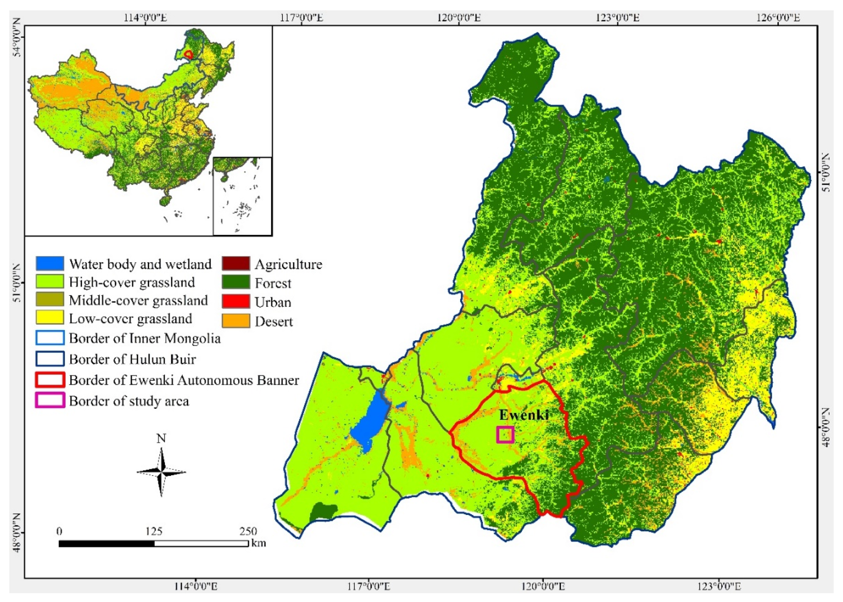
2. Study Area and Data Sources

2.1. Introduction of the Study Area

Hulun Buir is characterized by a meadow steppe (56.8%) and forest (34.6%) [43]. Grassland is the main land use type, which is used for livestock production, while arable land accounts for only 0.9% of the total land area [44]. Ewenki Banner is located in the northeastern part of Inner Mongolia and in the southeastern part of the Hulun Buir pasture (Figure 1), between 47° 32′ 50″–49° 15′ 37″ N and 118° 48′ 02″–121° 09′ 25″ E. It covers an area of 173.25 km from east to west and 187.75 km from north to south [43]. The annual mean temperature is from −2.4 °C to −2.2 °C with a rapidly increasing trend [45]. The annual frost-free period is 100–120 days. The general average annual rainfall is 350 mm with a decreasing trend, and annual evaporation volume is 1466.6 mm. Until 2013, its total land area was 1.87 million ha, including 0.65 million ha of forests (35% of total area) and 1.05 million ha of pastures (56% of total area); other land use types include dryland, water body, sand, etc. [43] From 2002 to 2012, the rural population in Hulun Buir increased from 858,400 to 1,200,600 [44].

Since 2011, the Chinese government has implemented a series of ecological restoration and ecosystem conservation policies (including a grassland eco-compensation policy) to protect and improve the natural grassland ecological environment, increase the income of herders, and establish modern grassland livestock. Ewenki Banner of Hulun Buir belongs to the forage-livestock balancing area. This area is characterized by high grassland productivity, slightly degraded or non-degraded grassland, relatively better natural conditions, and a strong ecological restoration ability. Through the adoption of forage-livestock balancing measures and the implementation of grazing suspension and alternative grazing within different planned areas, it is expected that grassland could gradually achieve the target of sustainable utilization. Economic loss due to reduced livestock in the forage-livestock balanced area will be compensated at 24 yuan/hectare (3.75 USD/hectare). Meanwhile, it is encouraged to build a livestock-breeding base with barns within a professional cooperation community or Gacha (Mongolian name for the village).

2.2. Data

The EcoC-G model in this study was developed mainly based on the household questionnaires survey data, from which the structures and running rules of agents in the ABM model were established. The household questionnaires were collected through face-to-face interviews of 85 herders in 2010 from June to July. The questionnaires include 3 parts, namely: (1) the structures of the households, including age, occupation, and education of family members; (2) the production and consumption of livestock, including species and total numbers of livestock, hay and fodder consumption, and willingness of herders’ livestock breeding; (3) income and consumption of herders, including income from animal husbandry, migrant work, government compensations or subsidy, and consumption expenses for daily life.

In addition, related census data, land use data, and NPP data were also used to support the study. The census data were obtained from the Social and Economic Statistical Yearbook of the Inner Mongolia Autonomous Region in 2010. These data were used to obtain livestock production, population, and education structures of households. The social data includes the family structure, ethnic customs, and social organization, which directly affect the agent’s evolution, career choice, and consumption structure (such as their main food being meat, and young people tending to work in the cities and refusing to live as herdsman like their parents). The data were obtained from the social survey and were input into the EcoC-G model. The detailed data analyzes the indices that are provided in the Appendix A. The land-use data was extracted from TM (Thematic Mapper) remote sensing images in 2010 and were used to initialize the spatial location of the land-use type in the starting year with a resolution of 100 m. The NPP data of grassland were computed using a VPM (vegetation photosynthesis model) model.

3. EcoC-G Model

The EcoC-G model used in this study is a newly developed model. It is developed from the repast example sugar model; the structure and method functions have referenced the mature agent-based models, including Bai et al.’s model [3] and Yan et al.’s model [10]. It is presented in accordance with the ODD + D (Overview, Design Concepts, Details, and Human Decision-making) protocol [46]. This protocol standardizes the description of the agent-based model and facilitates the comparison and communication of ABM scientists from different academic fields. For the full edition of the model described by ODD + D protocol, see Supplementary Material.

3.1. Overview

3.1.1. Purpose

The model was developed to simulate the ecological consumption process of herders from livestock production and daily life, by describing herders’ livelihood behaviors and responses to income, job opportunities, and grassland policy, as well as to predict the evolution of ecosystem pressure, livestock scale, and herders’ living levels under four pasture management scenarios to explore the possible win–win strategies for sustainable grassland management and to improve herders’ living level.

3.1.2. Entities, State Variables and Scales

Agents and grassland are the main entities. There are two types of agents in our model, including the individual herder agent and the herder’s household agent. In accordance with the family-contract responsibility system, China’s rural land property rights institution, the household is the basic unit of grassland management. Each household consists of several herder individuals. Individual agents are characterized by the following state variables: age, gender, education, living consumption, pasture income (the herding income of individuals), maxAge (the longevity of individuals), work income (the migrant work income of individuals), and occupation state (the occupation states of individuals). Household agents are characterized by the states of the following variables: family structure (age, gender, and occupation), livestock breeding (amount of livestock and consumption of ecosystem), household income (off-farm income and herding income), and owned grassland (area, supply of ecosystem, and grassland ecosystem pressure) (

Table 1. State variables of household agents.

Category	Variables	Explanation
Family structure	amountofFamilyM	the number of family members in each household
	individualAgent array	the array of family members
	children	the number of children in the family
	elder	the number of elders in the family
	parent	the role of parent in one family
	herders	the number of herders in the family
	outworkers	the number of workers out of the hometown in the family
Livestock breeding	sheepofCurrentYear	the number of sheep that the family is raising in the current year
	sheepofCurrentYearmiddler	the number of sheep that the family is raising in the middle of the current year
	sheepofLastYear	the number of sheep that the family raised in the last year
	sheepofLastYearmiddle	the number of sheep that the family raised in the middle of last year
	NPPsheepofCurrentYear (gC/(m2·a))	the NPP (net primary productivity) consumed by sheep herding in the family in the current year
	NPPsheepofLastYear (gC/(m2·a))	the NPP consumed by sheep the family herding in the last year
Household income	cashofCurrentYear (Chinese Yuan (CNY))	wage earnings by the outworkers in the family in the current year
	earnedofCurrentYear (CNY)	the sum of all of the earnings (off-farm income and herding income) in the family in the current year
	cashofLastYear (CNY)	wage earnings by the outworkers in the family in the last year
	earnedofLastYear (CNY)	the sum of all of the earnings (off-farm income and herding income) in the family in the last year
Owned grassland	amountofLand	the number of grassland plots that each household had
	familyLand array	the array of farmland plots planted by each household, stored information of each plot
	NPPproduceofCurrentYear (gC/(m2·a))	the NPP produced by the family in the current year
	NPPpeopleofCurrentYear (gC/(m2·a))	the NPP consumed by the family members in the current year
	NPPproduceofLastYear (gC/(m2·a))	the NPP produced by the family in the last year
	NPPpeopleofLastYear (gC/(m2·a))	the NPP consumed by the family members in the last year
	NPPEofCurrentYear (gC/(m2·a))	the real NPP pressure index in the current year

).

The grassland spatial information is included in this model as the basic context. Landscape cells are characterized by the following state variables: coordinates, land use type, NPP, land owner (household family), and ecosystem pressure (the value of ecosystem press of the cell). In the model, 1 time step represents 1 year (the temporal resolution); the spatial resolution is 100 m × 100 m (1 ha) and the length of the period is 30 years. The total study area is 400 km² (20 km × 20 km) (Figure 2).

3.1.3. Process Overview and Scheduling

At the beginning of each simulation, all herder household agents are randomly allocated with different spatial plots. Each household has multiple pasture plots, and one individual agent corresponds to 24 pasture plots (according to the household survey, each individual herder has an average grassland of 360 mu or 24 ha, i.e., occupying 24 plots under the spatial resolution of 1 ha in this model). Once the plots distribution is finished, the number of plots owned by one herder family agent remains unchanged. However, a household may rent plots from other household agents. At each time step, the household agent variable was executed first to drive its individual agents to an updated age and to run the individual status to the transfer sub-model to determine the occupation and education for each individual agent. Second, the land-use decision sub-model is executed to determine the type and number of livestock. Third, the ecosystem services consumption sub-model is executed to compute the ecosystem services consumption of the household and the ecosystem pressure of plots that are owned by the household. After all of the household agent variables were executed, the spatial environment sub-model was executed to show the service consumption pressure index visually on the land-use map. Within the model, the execution sequence for each time step is fixed, which is the same as that described above.

3.2. Design Concepts

3.2.1. Theoretical and Empirical Background

(1) General concept

This model measures the grassland ecological pressure by linking the supply and consumption of the grassland ecosystem service with the ecosystem’s NPP.

The reasonable ecosystem NPP consumption is defined as the human-consumed NPP to satisfy a substantial livelihood without producing excessive pressure on the ecosystem. The maximum NPP consumption carrying capacity is the actual NPP supply of the ecosystem; the living NPP consumption refers to the NPP that is consumed to obtain the necessary food (including grains, vegetables, meat, milk, and products, etc.; “necessary food” in this paper means the amount and type of daily food intake that is regulated in the Chinese standard of dietary nutrition balance.).

NPP supply and consumption: The NPP supply is calculated by the product of the estimated ecosystem NPP from the remote sensing model and the proportion that is utilized by the livestock. According to the previous study in the meadow grassland, the NPP available for livestock is 14% [47]. The NPP consumption consists of the livestock’s production consumption and the herders’ living consumption. Livestock production-consumption means the NPP that is consumed by the forage, which is needed for raising livestock. Therefore, the livestock production that is consumed NPP is calculated by the following equation:

$$\mathrm{ConsumedNPPg}=\mathrm{NUM}\times \mathrm{GW}\times \mathrm{GD}\times \left(1-\mathrm{MC}\right)\times \mathrm{Fc}$$

(1)

where NUM is the number of livestock that is raised by the household agent; GW (g) is the quantity of hay consumed per livestock per day; GD (g) is the number of annual hay-consuming days, which is 365 days for non-marketed livestock and 180 days for marketed livestock; MC is the water content of hay, which is 15% in this research [48]; and Fc is the converting factor from plant biomass (g) to carbon content (gC), with F_C as 0.45 in this research [48].

Since the living NPP consumption for a herder family to obtain an equal amount of livestock production income varies among the regions and production patterns, the NPP consumption for an equal amount of living consumption is also different. We developed a price equivalent parameter of NPP consumption (ρ), which measures the quantity of NPP consumed per RMB income, which is derived from different livestock production modes in different regions. Therefore, the living NPP consumption could be estimated by the product of the ρ value and the expenditure on food by the household.

ConsumedNPP_l = ρ × EXP_l

(2)

where the ConsumedNPP_l (gC/(m²·a)) is the NPP consumed for living consumption, ρ is the price equivalent parameter of NPP consumption, and EXP_l (CNY) is the economic expenditure for herders’ food demand; ρ is calculated as Equation (3):

ρ = ConsumedNPPg/PRODg

(3)

The income from livestock production PRODg (CNY) is calculated from the number (NUMc) and price (PRc) of various kinds of newborn animals in the year. The yield of wool (WOOLo) and price (WOOLp) is calculated by the following Equation (4):

$$PRODg=NUMc\ast PRc+WOOLo\ast WOOLp$$

(4)

Food expenditure FOODex (g) is calculated from the consumption of grain, meat, and milk (FOODe, MEATe, and MILKe and their respective prices FOODp, MEATp, and MILKp (CNY)) and is calculated by using the following Equation (5):

$$FOODex=FOODe\ast FOODp+MEATe\ast MEATp+MILKe\ast MILKp$$

(5)

In the above calculation equations, livestock production output data come from the questionnaire survey, and the price comes from the Inner Mongolia Social Economic Statistical Yearbook of the same year.

The Ecosystem Pressure Index (EPI): The EPI means the degree of ecosystem pressure caused by ecosystem consumption in the research area, which is calculated by the ratio of the production-consumption (ConsumedNPPg) to the NPP supply (SupplyNPP).

$$\mathrm{EPI}=\frac{\mathrm{ConsumedNPPg}}{\mathrm{SupplyNPP}}$$

(6)

(2) Hypotheses

There are two hypotheses in our study. (i) During the model running time, grassland productivity was stable, and there was no man-made grassland generated. (ii) During the simulated years, the running rules of the model remain unchanged. The model parameters of grassland area per capita, migrant work salary, prices of livestock, and the prices of land rent were fixed.

(3) Empirical background

Our model is based on the local truths, and the data are collected from first-hand questionnaire surveys. We use the survey data to analyze the characteristics of individuals and households in the real-society and use a probability method to build the rules of the EcoC-G model, to effectively model agents’ behaviors in an artificial-society.

3.2.2. Individual Decision-Making

The EcoC-G model includes multiple decision-making levels. The individual agents decide their own individual states, and the agent’s decisions influence the household’s livelihood strategies and structures. The household agents decide the pasture and livestock management, and their decision influences grassland utilization which, thus, impacts ecosystem consumption. This decision-making is simulated for each pasture plot while the behaviors of herder individuals and families are simulated for each agent. In the model, as individual agents grow older, their states change correspondingly. The changing individual agent choice on occupation, family livestock production, and family food consumption would all affect the decision of the household agents and impact the household livelihood, such as the marketing rate of livestock or pasture renting. Based on the interview questionnaires, for instance, if there is no labor work in livestock production for a family, the raised livestock should all be sold. If the answer is yes, there is labor work in livestock production, then normal livestock production can go on. A detailed explanation is shown in the section “Household livelihood decision sub-model”.

3.2.3. Learning

Both household agents and individual agents could improve their ability to achieve objectives by learning from the decision-making behaviors and effects of other agents’ decisions. Through learning, the household agents are able to improve decision-making in livestock breeding for pasture protection and a higher living level. Through learning, the individual agents could increase their income and improve their ability for livestock breeding. Collective learning is implemented in the model, and households with the same agent occupation state, family livestock production, and family food consumption will share the same rules of decision-making.

3.2.4. Individual Sensing

Individuals are assumed to sense and consider their age, occupation, and economic development. Households are assumed to sense their livelihood structure, economic development and consumption pattern. With sensed information, both household agents and individual agents can improve their ability to adjust their decision-making.

3.2.5. Individual Prediction

With the aging of herder individual agents in a new year, agents would decide to choose their occupation state based on the transfer rules that were obtained from the household survey; for instance, at the age of 18, 60% of individual agents that graduated from high school would enroll in colleges or universities by stochastic allocation and prediction (detailed state and transfer rules provided in Section 3.3.4 sub-model (1), individual transferring sub-model), and the herder families would determine the living consumption according to the income from livestock production or off-farm work.

3.2.6. Interaction

The interactions between households and plots are direct. The interactions between individuals and plots are indirect, and individuals have to interact with plots with the help of the household that they belong to.

3.2.7. Collectives

The household agent is the basic unit of the EcoC-G model, and the individual agent who comprises the household agent is the smallest unit of the model. The households with the same occupation states and structures would share the rules for an individual occupation choice, family livestock production, and family food consumption. These rules are imposed by a modeler and were achieved from the household survey data. For instance, by counting family members in each household, this model allocates the same number of plots to each household. The plots that were owned by the same household were distributed adjacently.

3.2.8. Heterogeneity

The individual agents and household agents are heterogeneous. The occupation states are different for the individual agents, the production and consumption are different between the household agents, and the ecosystem consumption of households are heterogeneous during their decision-making process (see Section “Descriptions of Sub-models” for more detail).

3.2.9. Stochasticity

The individual member structure of household agents is created proportionally according to the household survey, and it ensures the consistency of family structures based on age, gender, occupation, and so on, between the modelled proportion and the actual survey proportion. The plot locations of each household are distributed stochastically in the model. During the processes of production, the decisions of household agents and the occupation selection of individual agents, the agents’ behaviors are all changed stochastically within certain interval ranges.

3.2.10. Observation

The output from the simulation includes the living consumption NPP per capita, livestock numbers in the middle and at the end of the year per capita, ecosystem consumption pressure, and the total population in the region. The desired emergence includes the reasonable living level for the people based on a balanced ecosystem NPP supply and consumption relationship.

3.3. Details

3.3.1. Implementation Details

This EcoC-G model was developed with the Java language in the RePast simulation platform. Considering the existence of random parameters in the model, each scenario would be simulated 50 times, and the average values of the 50 times would be taken as the model output data.

3.3.2. Initialization

The initial state of the model was determined according to the household survey and social economic statistical data. Main initializing parameters are in

Table 2. The initialization of the main parameters in the model.

Parameter	Initial Value	Source
The average population of households	3.2	Field survey and statistic yearbook of Inner Mongolia
Amount of family member (percent, number)	4%, 1	Statistic yearbook of Inner Mongolia
	10%, 2
	40%, 3
	42%, 4
	4%, 5
Educating of individual (represent number, education level)	1, highest with primary education 2, middle school 3, high school 4, university and upper	Statistic yearbook of Inner Mongolia
Age of individual	0–100 (maximum age randomly distributed in 60–100)
Pasture area per capita (hm2)	24	Field survey and statistic yearbook of Inner Mongolia
Ecological compensation (¥(CNY)/hm2)	45	Field survey
Number of sheep per sheep-breeding family	101	Statistic yearbook of Inner Mongolia
Number of cattle per cattle-breeding family	22	Statistic yearbook of Inner Mongolia
The upper limit for breeding ((number of sheep)/person)	500	Field survey
Income of flexible working per family (¥(CNY))	15,000	Field survey and statistic yearbook of Inner Mongolia
Income of breeding per family (¥(CNY))	43,000	Field survey and statistic yearbook of Inner Mongolia
Food consumption amount per capita (¥(CNY))	2654	Field survey and statistic yearbook of Inner Mongolia
The ratio of livestock number in the middle to that at the end of the year	0.62	Statistic yearbook of Inner Mongolia

, other important initializing perimeters can be found in the Appendix A. The agents running space is a two-dimension grid with land use information as the background. The spatial resolution of land use data is 100 m. Model initializations include spatial environment initialization, household agents’ initialization, and individual agents’ initialization. The initialization of the household agents includes structures of ages, labor, family members, and livestock. The livestock data is obtained from the statistic yearbook of Inner Mongolia, and we converted one cattle to 5 sheep according to their forage requirement [49] to normalize all the livestock of the households. The initialization of the individual agents includes the initializations of the occupations, education status, and genders of each herder individual; the initialization of the running space includes the allocation of plots for each household.

The initialization is not always the same. With the stochasticity of the individual member structure of household agents, the plot locations of each household and the occupation selection of individual agents, the initializations are different each time.

3.3.3. Input Data

The input data were obtained from the social survey and spatial data. Social survey data include the population distribution of households, the age distribution of farming or livestock family members and the occupation status distribution of farming or livestock family members (detailed descriptions are in the Appendix A). Spatial data include land-use data and the NPP data of grassland.

3.3.4. Sub-Models

The model includes three sub-models, namely, individual status transferring sub-model, households’ livelihood decision sub-model, and ecosystem pressure sub-model.

The framework of the EcoC-G model has been shown in Figure 3. The individual status transferring sub-model outlines the transition between different individual states, and the individual agents’ behaviors include choosing their occupation type and consumption pattern. The household livelihood decision sub-model mainly simulates family livestock production and family consumption. Different consumption patterns will intake different types of food and then generate different NPP consumptions. The household agents’ behaviors include choosing the livestock amount, grassland use, and computing their income, payments, and NPP consumption. The ecosystem pressure sub-model would compare the supply NPP of the ecosystem and the consumption NPP by individuals and livestock, resulting in the ecosystem pressure of its grassland.

(1) Individual status transferring sub-model

There are 7 individual states according to the education and employment situation of surveyed households, namely: (1) The fostered state, meaning that the agent is in infancy or in primary or middle school; (2) the educated state before employment, meaning the agent is accepting vocational training or university education; (3) the herder state, meaning the agent is working as a herder; (4) city worker with odd job state, meaning the agent is a migrant worker in an urban area and engages in odd jobs; (5) city worker state with permanent employment, meaning the agent is working in a state-owned enterprise or government in the city; (6) the rural dependent state, meaning the agent has lost the ability to work or live in a rural village; and (7) the retired state, meaning the agent has retired from being a city worker and is sustained by a retirement pension. According to the analysis of survey data, the transitional relationship for individual agent state is shown in Figure 4, where S represents the state of individual agents and Rij represents the rules that should be followed while transitioning from status i to status j. The transition rules between different individual states were derived from the questionnaire survey data and are listed in the Appendix A.

For the natural (birth/death) and social (emigration/immigration) population changes in the model, we firstly initializing the individuals and households. Different households initially consist of different kinds of individuals (specific structure could be found in Appendix A,

Table A2. Occupation status distribution of farming or livestock family members.

Population Per Family	Hulun Buir
1	Livestock, male
2	1 family: 1 old, 1 adult; 2 families: elderly couple over 60; 2 families: middle-aged couple engaged in farming
3	17 families: 1couple + 1 child, couple engaged in breeding, 12 children in school, 2 children being migrant worker, 3 children in breeding; 2 families: 1 old + 2 children; 1 family with 1 couple + 1 old; at least two persons in breeding, 1 as migrant worker, in breeding or school for the latter three families
4	19 families: 1 couple + 2 children, couples all engaged in breeding, 7 families with two students, 3 families with 1 student and 1 migrant worker, 4 families with 1 student and 1 child in breeding, 2 families with 2 young migrant workers, 1 family with 2 children in breeding, 2 families with 1 young migrant worker and 1 child in breeding; 1 family with 1 old + 1 young migrant worker+ 2 children in breeding; 2 families with 1 old + 1 couple + 1 child in school, the other three in breeding
5	1 family: 1 old + 4 adults, in breeding; 1 family: 1 one couple + 1 adult couple + 1 child in school, the other four in breeding

). We assumed that if there are young couples with the most suitable ages for childbearing (20–23), and they also have a good economic condition (the household income for the year is more than 10,000 CNY), then a new baby will be born, and the total population will increase by one. If the age of the individual is in the range of 60–100, then there is a random probability of death. In this model, we didn’t consider the emigration/immigration from regions beyond the study region. The population of herders is changed with income. When the average income of outworkers is lower than the average income of farmers, the outworkers would return to farmland and become a herder, and vice versa.

(2) Household’s livelihood decision sub-model

The household livelihood decision sub-model is mainly used to simulate the individual agent occupation choice, family livestock production, and family food consumption.

In the model, the first decision is about the career choices for the individual agents, and the second decision is about family livestock production. If there is no labor work in livestock production for one family, the raised livestock should all be sold. If yes, normal livestock production can go on. The livestock quantity of the herder family can be calculated by the reproduction rate (β) and marketing rate (μ), which are respectively defined as follows:

$$\beta =\left(\text{NUM-MID}i-{\text{NUM-END}}_{\mathrm{i}-1}\right)/{\text{NUM-END}}_{\mathrm{i}-1}$$

(7)

$$\mu =\left(\text{NUM-MID}i-{\text{NUM-END}}_{\mathrm{i}-1}\right)/\text{NUM-MID}i$$

(8)

wherein NUM-MID_i is the livestock number in the middle of the ith year; and NUM—END_i−1 is the livestock number at the end of the (i−1)th years.

According to the survey in the research area, a reproduction rate is commonly in the range of (0.4, 0.8). The marketing rate is in the range of (0.4, 0.6) according to the statistical yearbook data in Inner Mongolia. In the decision-making sub-model, the reproduction rate is a random number from the range of (0.4, 0.8). However, the marketing rate (μ) is affected by the policy, environment, and family labor force, which is defined as follows:

$$\mu =\{\begin{array}{l}1\\ Random\left(0.4,0.6\right)+k\end{array}\begin{array}{cc}& \end{array}\begin{array}{l}if \mathrm{k}=1\\ if \mathrm{k}\ne 1\end{array}\}$$

(9)

wherein k is the impact factor, which is concerned with the policy factor kp, the environmental factor ke, and the labor factor kf.

The respective values of the above three factors are defined as follows:

$$kp=\{\begin{array}{l}Random\left(0, 0.1\right)\\ Random\left(-0.1, 0\right)\end{array}\begin{array}{cc}& \end{array}\begin{array}{l}having.policies\\ no.policies\end{array}\}$$

(10)

In Equation (10), if there are ecological competition policies provided for the households, the value of kp is a random datum and the interval is (0,0.1), which means the marketing rate is increased; otherwise, the interval is (−0.1,0), which means the marketing rate is decreased.

$$ke=\{\begin{array}{l}Random\left(0, 0.1\right)\\ Random\left(-0.1, 0\right)\end{array}\begin{array}{cc}& \end{array}\begin{array}{l}if.SupplyNP{P}_{i-1}<{\mathrm{ConsumedNPP}}_{\mathrm{g}i-1}\\ if.SupplyNP{P}_{i-1}\ge {\mathrm{ConsumedNPP}}_{\mathrm{g}i-1}\end{array}\}$$

(11)

In Equation (11), if the SupplyNPP (gC/(m²·a)) in the last year is less than the ConsumedNPPg (gC/(m²·a)) in the last year, the value of ke is a random data and the interval is (0,0.1), which means the marketing rate is increased; otherwise, the interval is (−0.1,0), which means the marketing rate is decreased.

$$kf=\{\begin{array}{l}1\\ Random\left(0,0.1\right)\\ Random\left(-0.1,0\right)\end{array}\begin{array}{cc}& \end{array}\begin{array}{l}if.0 \mathrm{herdsman}\\ if.\mathrm{herdsman} \mathrm{decrease}.\mathrm{but} \mathrm{not} \mathrm{be} 0\\ if.\mathrm{herdsman} \mathrm{increase}\end{array}\}$$

(12)

In Equation (12), if the household agent has no herdsman, the value of kf is 1; otherwise, if the amount of the herdsman in the household agent is decreased and not equal to zero, the value of kf is a random datum and the interval is (0,0.1), which means the marketing rate is increased; otherwise, the interval is (−0.1,0), which means the marketing rate is decreased.

The value of k is defined as follows:

$$k=\{\begin{array}{l}1\\ kp+ke+kf\end{array}\begin{array}{cc}& \end{array}\begin{array}{l}if.kf=1\\ if.kf\ne 1\end{array}\}$$

(13)

In Equation (13), if the household agent has no herdsman, the value of kf is 1, the value of k is 1, and the value of μ is 1 in Equation (9), which means all of the livestock will be sold because of lacking a herdsman; otherwise, the value of k is the sum of the three parameters.

The value of the marketing rate μ is not only determined by the above formula but is also affected by different simulation scenario conditions, which will be introduced later. The quantity of livestock NUM-MIDi in the ith year is calculated as follows:

$$\text{NUM-MID}i=\left(1+\beta i\right)\ast \text{NUM-ENDi}-1$$

(14)

The number of livestock marketed in the ith year is calculated as follows:

$$\text{NUM-SOLD}i={\mu }_i\ast \text{NUM-MID}i$$

(15)

The remaining livestock number at the end of the ith year is calculated as follows:

$$\text{NUM-END}i=\left(1-{\mu }_i\right)\text{NUM-MID}i$$

(16)

The living decision of herder families would determine the living consumption level for the whole year. The herder families would determine the living consumption according to the income from livestock production, as follows:

• When the income of livestock production is less than the life consumption demand, the livestock production income cannot support the lives of herder families, and all of the livestock production income will be used for the living consumption.
• When the livestock production income is more than, or equal to, the living consumption demand, the livestock production income is able to support all of the lives of herder families. The whole living consumption of the herder families comes from livestock production; i.e., the consumption is equal to the demand. The living demand is set with a reference to the resident nutrient balanced standard dietary amount [50].

(3) Ecosystem pressure sub-model

The ecosystem services consumption sub-model simulates the change occurring to the ecosystem services consumption and the EPI. In this study, the supply of the ecosystem service is assumed to be stable and is set to the average NPP value in the past 20 years. The ecosystem services consumption and the EPI are calculated by Equations (1), (2), and (6).

4. Scenarios and Simulation

Four scenarios were designed according to the current state and possible future development trends of the grassland management in the research region to simulate the herders’ livelihood and ecosystem pressures for the next 30 years under each scenario of the four grassland management goals, with a time step of one year. Under each scenario, the ecosystem pressure would be changed with herders’ response to the presumed livelihood goals and ecological protection policy by adjusting the livestock marketing rate (μ_i):

(1) Scenario 1: The current situation.

This scenario is used to simulate the ecosystem consumption and its pressure over the next 30 years in the case where there is no change occurring in the current situation of livestock production and in the living consumption state. In scenario 1, μ_i = μ₀. According to the analysis of survey data, μ₀, the average annual marketing rate of the local livestock is 0.38.

(2) Scenario 2: Preference for the improvement of the herders’ living levels.

The herders aim to accumulate wealth and to improve their living level. The parameters are set as

Table 3. The parameters of the scenario 2.

Parameters	Conditions	Value or Intervals of Parameters
μi	$\mathrm{ConsumedNP}{\mathrm{P}}_{\mathrm{si}-1} < \mathrm{ConsumedNP}{\mathrm{P}}_{\mathrm{lb}}$	<0.7μ0
	$\mathrm{ConsumedNP}{\mathrm{P}}_{\mathrm{si}-1} \ge \mathrm{ConsumedNP}{\mathrm{P}}_{\mathrm{lb}}$	<0.8μ0
kp	No ecological compensation	kp = 0

.

The parameter ConsumedNPP_si−1 (gC/(m²·a)) means the sold livestock production consumed NPP in the (i−1)^th year. The parameter ConsumedNPP_lb (gC/(m²·a)) means the basic NPP consumed for living consumption (the Chinese standard of dietary nutrition balance); kp = 0 means the government does not provide compensation for the household. If ConsumedNPP_si−1 < ConsumedNPP_lb, which means the income from the sold livestock production does not meet the basic living consumption, then the value of the marketing rate μ_i is in the interval of [0,0.7μ₀]; otherwise, the value’s interval is [0,0.8μ₀]. Therefore, in this scenario, the amount of livestock is increased continuously because of the lower marketing rate, and the household’s wealth is raised, too.

(3) Scenario III: Preference for the protection of the grassland ecosystem.

The top priority of herders is to protect the ecosystem, and the living consumption of the herders is limited within the NPP supply capacity of the ecosystem. The parameters are set as

Table 4. The parameters of scenario 3.

Parameters	Conditions		Value or Intervals of Parameters
μi	$SupplyNP{P}_{i-1}>{\mathrm{ConsumedNPP}}_{\mathrm{g}i-1}$	$ConsumedNP{P}_{si-1}<{\mathrm{ConsumedNPP}}_{\mathrm{lb}}$	≤0.7μ0
		$ConsumedNP{P}_{si-1}\ge {\mathrm{ConsumedNPP}}_{\mathrm{lb}}$	≥1.4μ0
	$SupplyNP{P}_{i-1}\le {\mathrm{ConsumedNPP}}_{\mathrm{g}i-1}$	$ConsumedNP{P}_{si-1}<{\mathrm{ConsumedNPP}}_{\mathrm{lb}}$	≥1.5μ0
		$ConsumedNP{P}_{si-1}\ge {\mathrm{ConsumedNPP}}_{\mathrm{lb}}$	≥1.6μ0
kp	With ecological compensation		kp ranges between [0,0.1]

.

In scenario 3, the parameter ConsumedNPP_gi−1 (gC/(m²·a)) means the total livestock production consumed NPP in the (i−1)^th year. The parameter SupplyNPP_i−1 (gC/(m²·a)) means the total NPP supplied by the household agent’s grassland. The two parameters ConsumedNPP_si−1 (gC/(m²·a)) and ConsumedNPP_lb (gC/(m²·a)) are the same as the parameters in scenario 2. The total NPP supply and total livestock production of consumed NPP in the last year affect the decision on the marketing rate in the following year. Moreover, the sold livestock production consumed NPP is also compared with the basic living consumption NPP, and the result could decide the value interval of μ_i. in this scenario; the household agents have ecological compensation.

(4) Scenario 4: Aiming at a balance between the living level of the herders and ecosystem protection.

The preference of the agents is seeking the balance between improving their living level and protecting the ecosystem. On the condition that the ConsumedNPPg does not exceed the SupplyNPP by the ecosystem, the herders could keep increasing the number of livestock and improve their living level until reaching a new balance.

The parameters in scenario 4 are all the same as the parameters in scenario 3 (

Table 5. The parameters of scenario 4.

Parameters	Conditions		Value or Intervals of Parameters
μi	$SupplyNP{P}_{i-1}>{\mathrm{ConsumedNPP}}_{\mathrm{g}i-1}$	$ConsumedNP{P}_{si-1}<{\mathrm{ConsumedNPP}}_{\mathrm{lb}}$	≤0.7μ0
		$ConsumedNP{P}_{si-1}\ge {\text{Consumed-NPP}}_{\mathrm{lb}}$	≥0.8μ0
	$SupplyNP{P}_{i-1}\le {\mathrm{ConsumedNPP}}_{\mathrm{g}i-1}$	$ConsumedNP{P}_{si-1}<{\mathrm{ConsumedNPP}}_{\mathrm{lb}}$	≥1.2μ0
		$ConsumedNP{P}_{si-1}\ge {\mathrm{ConsumedNPP}}_{\mathrm{lb}}$	≥1.6μ0
kp	With ecological compensation		kp ranges between [0,0.1]

). The difference between them is the value interval of μ_i. The value intervals of μ_i in the four scenarios are determined through an adequate amount of model parameter testing.

5. Results and Analysis

5.1. Changing Trend of Ecosystem Consumption Pressure

Under the current production and management mode of livestock (Scenario 1), the Consumed-NPP does not exceed the NPP supply of the ecosystem. The EPI is less than 0.5 and has a decreasing trend (at year 30, the pressure drops to 0.2), which indicates that the ecosystem could never be overloaded, owing to the continual decline of the livestock number. The simulation result of the second scenario indicates that the pressure of the ecosystem has an increasing trend, and it becomes more stable in year 18, when the EPI climbs to 2.2. Over the last five years, it has a slowly decreasing trend (from 2.2 to 2.0) by virtue of the decrease of herdsmen labor (from 902 to 813) (Figure 5). This indicates that if there are no restrictions on the livestock number that is imposed on herders, the ecosystem consumption will exceed the supply of the ecosystem (with a maximum pressure of 2.3 times). Under Scenario 3, because of the strict restrictions on the livestock number, the ecosystem pressure decreases (by 0.1 and 0.2 at years 2 and 3, respectively) at first, but has a fluctuation trend within the range of 0.3. The simulation result of Scenario 4 shows that the ecosystem pressure has an increasing trend (from 0.4 at year 1 to 0.95 at year 8) in the beginning, and then keeps stable throughout the simulation period, with the variation range within 0.8.

5.2. Changes in Wealth Accumulated by the Herder Family

The herder households’ wealth is mainly reflected by the amount of raised livestock. The simulation result of scenario 1 shows that the livestock number of each family in the middle and at the end of the year has a downward trend (decreased from 130 to 80, and 80 to 50, respectively), which indicates that if the execution of the current ecological management policy is continued, the income of local herders will have a continued downward trend.

The simulation result of scenario 2 shows that in the beginning, the number of livestock keeps rising. Until year 19, the number of livestock reaches the upper-limit capacity of the herdsman laborers (the number of livestock in the middle of the year and at the end of the year were 778.8 and 483.8, respectively), and the number of livestock raised by each herder household is maintained at 500–800, which is equivalent to 5 times the current breeding stock (Figure 6). To accumulate wealth, from year 1 to 19, the marketing rate of livestock remains at a low level (0.3–0.4) (Figure 6), so the accumulating rate of the livestock amount at the end of the year is higher than in the middle of the year. This indicates that, if there is no restriction on the livestock scale, herders usually do not consider the overgrazing impact on pasture, and the wealth of herders can reach a very high level.

The simulation result of scenario 3 shows that the average number of livestock raised by each herder’s labor has a rapid downward trend (94.6 in year 1, and 13.8 in year 5), and it will drop to a very low level and fluctuate around this level after 5 years. The number of livestock in the middle of the year is approximately 22, while the number of livestock at the end of the year is approximately 8 in year 5. For each herder household, the income from livestock production is very low.

The simulation result of scenario 4 shows that the average number of livestock raised by each herder’s labor has a stable upward trend (129.6 in year 1, and 280.2 in year 30) and maintains a relatively stable state. The number of livestock in the middle of the year is approximately 280, while the number of livestock at the end of the year is approximately 173 in year 30. Under this scenario, the wealth of each herder is higher than under scenarios 1 and 3 and maintains a stable high level (Figure 6).

5.3. Changes of Herders’ Living Status under Four Scenarios

We use NPP consumption for basic food as living consumption and take the amount of food per capita in the dietary standard (5000 gC/a) as the minimum demanded quantity of the rational ecological consumption [51]. According to the simulation results (Figure 7), the herders’ living can achieve basic living standards over the next 30 years under scenarios 1, 2, and 4 (Figure 7, the living consumption of the three scenarios are higher than 5000 gC/a), i.e., their income from animal husbandry can support their basic living consumption. Under scenario 3, the herders’ living consumption has a sharp volatility (Figure 7, the living consumption of the scenario 3 is lower than 5000 gC/a), which is because there is too much emphasis imposed on the protection of the ecosystem, and the herder households have to reduce the number of raised livestock. The result indicates that the herders’ living will be greatly influenced, and their living quality will not be guaranteed in scenario 3 (Figure 7).

The marketing rate is a key index that reflects herders’ behavior to adjust livestock scales. Under the no-policy scenario 2, the marketing rate is always lower than the current value (38%). Especially during the first 12 years, it remains below 30%. Then, it has a gradually increasing trend by 2% (37–39%) and reaches a new steady state at 39%. The reason is that the herder’s labor can increase the breeding amount and reduce the marketing rate to accumulate wealth until reaching the maximum breeding amount. In scenario 3, the marketing rate has a highly fluctuating trend (increasing from 0.3 in year 1 to 0.6 in year 6, decreasing from 0.4 in year 9 to 0.3 in year 15, and increasing to 0.4 in year 30). To respond to ecological protection policies, the herder households reduce the number of raised livestock by selling many livestock to lower the ecological pressure. Through highly reducing the raised livestock number for 8 years continuously (the marketing rate is maintained at 50–60%) (Figure 7), the livestock breeding stock begins to reach a stable minimum point. Then, the marketing rate begins to rapidly decline until year 12 (30%) and increases to a stable status (35–40%) between year 18 and year 30. In scenario 4, to seek a more modest regulation measure to realize the rational ecological consumption, the marketing rate was adjusted from 30% to 45% and lies in a relatively balanced state. When the ecological consumption is greater than the ecological supply, the marketing rate will have a greatly increasing trend (≥1.2*μ_avg), whereas when the ecological consumption is lower than the supply or even the basic living consumption, the marketing rate will have a downward trend (≤0.7*μ_avg).

6. Discussion

6.1. The Promotion and Limitation of the EcoC-G Model

With the goal to express the behavioral and environmental mechanisms that create the organization and structure of artificial society, ABM is designed from bottom to top to simulate the interactions of individual agents. This kind of structure was proven to be effective in deepening the understanding of driving factors, changing process and spatial characteristics on land use change [52], socio-ecological systems [53], and environmental protection [37]. However, the pattern of modeling social–ecological systems is still being explored. Some studies are trying to implement a loose coupling approach to combine ecosystem models with ABM, for instance, Robinson et al. loosely coupled the ecosystem process model BIOME-BGC (BioGeochemical Cycles) with ABM and successfully linked the land-decisions to carton storage, however, it still contains many computational tasks and also needs strict assumptions to link two models [54]. The EcoC-G model we constructed in this study links the grassland ecosystem supply with social system consumption by NPP indicator, which shows a direct interaction simulation in a social–ecological system. It also employs the EPI to achieve the cross-scale simulating result, from households’ living consumption to regional ecosystem pressure, which is essential for sustainable land-use options research.

To model agents’ behavior, empirical characterization and parameterization are necessary, however, it is a major challenge to refine and assess the differentiated behavior through empirical observation [53]. Some studies set the household as a basic agent unit, which would miss land use information within the household [33]. Some others only use census data to classify the household types and to simplify the model [55], however, it loses the practical and social meaning of behavioral description. There are lots of methods that are helpful for extraction of behavior characteristics from the real world and which achieve the parameterization, such as household surveys, expert knowledge, interviews, and participant observation [56]. In our study, we combine the household survey and census data to extract agent classification and characterization, and set individuals as the minimum unit and household as the decision unit to achieve a more practical and robust simulation. This study is still a beginning trial for sustainable ecological consumption modeling by incorporating the mechanism of NPP consumption in a grassland ecosystem into an agent-based model. Based on this, we would construct and develop new supply-consumption relationship models by understanding the interaction mechanism between human consumption activity and the related ecosystem services.

6.2. Exploring the Possibility of a Balanced Land Management Method on Grassland Ecosystem

According to the simulation results in scenario 1 and 3, where the grazing control exists to different extents, the livestock amount would decrease and herders would not be able to achieve basic living standards in scenario 3 with strict constraints. The decreasing livestock strategy corresponds with the reality, according to the field survey analysis by Du et al. [16], however, Du et al.’s study also points out that with the grazing control policy, household dependence on grassland is also decreased; diversification of income source would ensure the basic living standard of local households. In our study, we only focus on the relationship of grassland ecosystem supply and consumption, and we acknowledge that under strict grazing control, the production from grassland cannot meet the basic living needs of households. More factors, such as precipitation and the multiple choices of herders’ livelihood means, and perspective for this social-ecosystem, would be developed in the next step.

One of the most prominent features of ABM is the initiative of agents. Because of this initiative, the agents, specifically the herders in the EcoC-G model, have the ability to perceive and learn, so they can actively adjust their livelihood behaviors, such as animal husbandry production and living consumption level, and explore a mode to meet their needs based on their willingness and also under the capacity of ecosystem. This is a feature that is not available in other statistical models or process models, and it provides the possibility for real simulation and exploration.

6.3. The Validation of the EcoC-G Model

Verification and validation for ABM models were always taken as a challenge for model development [53]. In this study, we tried to ensure the validity of this artificial society model by calibrating the rules of agents’ behaviors and the interactions between agents and environments with actual society. Firstly, the basic rules of agents’ behavior in our model are exactly and strictly extracted from the local practices. We combined the household survey and census data to extract agent classification and characterization. To simulate behavioral responses of humans, the empirical data are required. It helped us to develop the behavioral categories and scaling to the whole population of agents. We conducted in-depth interviews with 85 households, randomly, to ensure they were representative, and collected information concerning household structure, household livestock production and consumption, and herders’ income and consumption through the interview. Based on this information, we categorized the households behavior. Then, combined with the census data of Ewenki Autonomous Banner, we initialized the distribution and quantification of households and livestock, and achieve upscaling to the whole study region. Secondly, we set individuals as the minimum unit, which corresponded with one pixel of land, and set household as the decision unit in accordance with the family-contract responsibility system in China. These agents’ definition and operation mechanism avoided missing the household internal land change condition and were closer to reality, thus, ensuring a practical and robust simulation. Thirdly, according to the comparative results in Section 6.2, specific to the aim of our study to only focus on the grassland ecosystem supply and consumption, our results are consistent with field survey results in Inner Mongolia.

The model in our study is an artificial-social model, which is constructed based on the mechanism and running rules in accordance with local facts. Although this model cannot achieve simulation of all factors in the social–ecological system, but rather concerns the key issue, namely, the impact of farmers’ livelihood behavior on grassland ecosystem pressure, the rules of agents behavior and the mechanism of impact between agents and environment have substantial practical evidence. Thus, this model can support the policy-making process in complex social–ecological systems.

7. Conclusions

In this paper, we developed an EcoC-G model to simulate the effects of herder’s livelihood behaviors on ecosystem pressure and used the grazing control area Hulun Buir grassland in Inner Mongolia as an example to simulate the effects of designed land use options on the evolution of the ecosystem and human well-being.

(1)

The EcoC-G model was properly developed by simplifying the factors and mechanisms of the social–ecological system to obtain a more direct and explicit relationship between grassland ecosystem supply and herders’ consumption. This model links the supply grassland ecosystem and social system with an index of ecosystem pressure. This index measures the balance status between grassland productivity and husbandry development demand by calculating the ecosystem’s NPP supply and the herder’s NPP consumption from livestock. The NPP consumption was changed with the herder’s livelihood strategies, while the livelihood strategies were determined by the age structure, occupation structure, and pasture of the herder’s family. Therefore, the mechanism of this model provides a new cross-scale way to scale the grassland use behaviors at the household scale to meet the ecosystem pressure at the regional scale.

(2)

In this model, the herder agents have the initial ability to observe natural and policy environments, and have the ability to perceive and learn about livelihood strategies from other agents. Therefore, the herder agents can adjust their livelihood behaviors to adapt to the ecological protection policy, while the indices of ecosystem pressure and herders’ living standards were simultaneously calculated to observe the effects of grassland use on the ecosystem and human well-being. Therefore, this model could be a practical tool to guide scientific decision-making for grazing management, to seek a win–win approach to ensure sustainable grassland use and to improve herders’ livelihood.

(3)

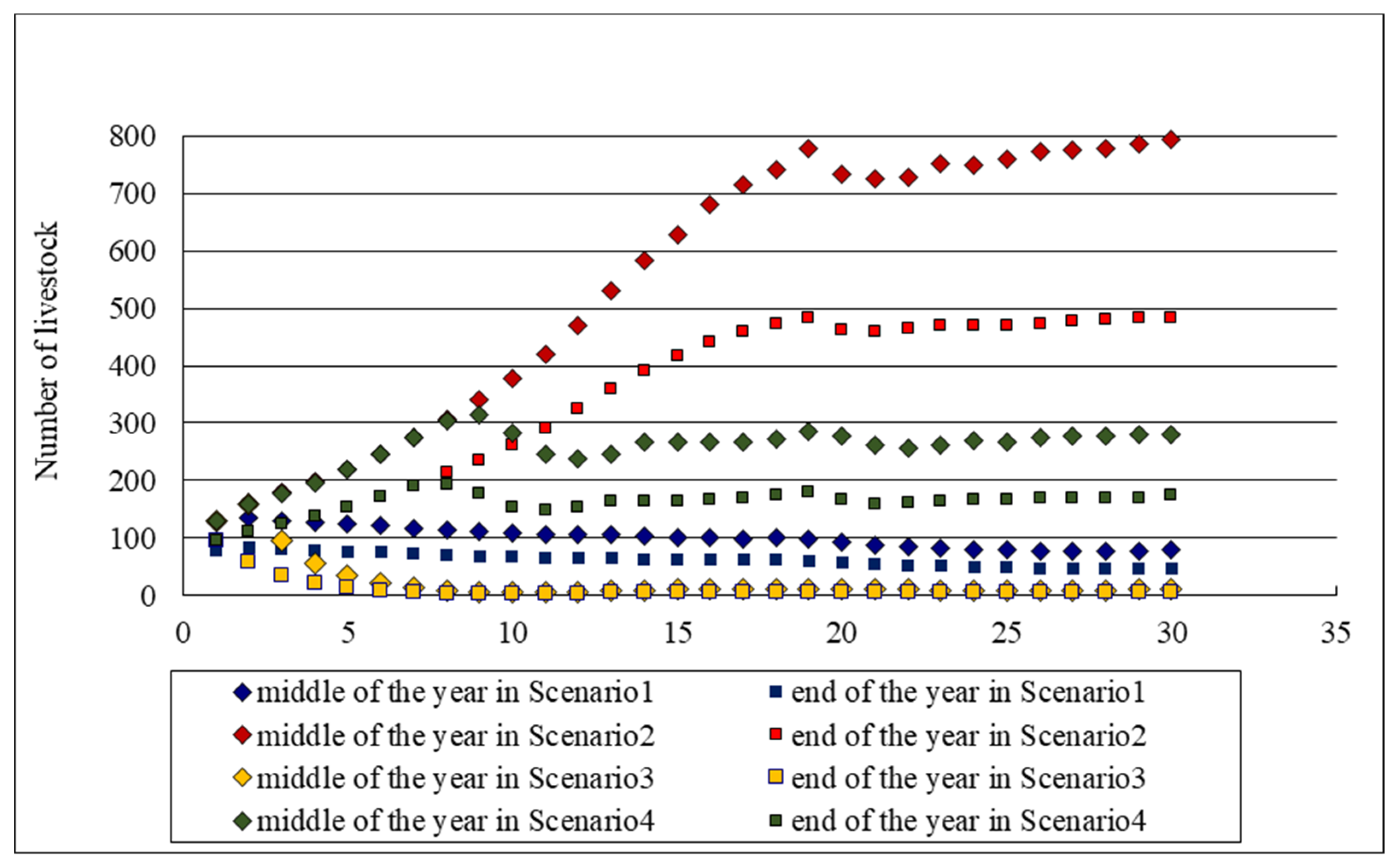
According to the simulation results of 4 scenarios, under the current grassland management mode, the pasture could never be overgrazed, and herders could achieve the basic living standard, but the accumulated wealth would be decreased due to the continual decline of the livestock amount. If no grazing control was imposed on herders, herders could accumulate wealth by increasing the breeding amount (approximately 5 times greater than the current mode) and reducing the marketing rate, but the ecosystem consumption pressure would reach a maximum of 2.3 times. With strict restrictions on the livestock number, the pressure on the ecosystem decreases; however, herders cannot achieve the basic living standards and accumulate wealth with limited livestock. Under the balance-oriented scenario, timely and gentle grassland management strategies (i.e., adjusting the breeding scale of livestock) were implemented, modest regulation led to rational ecological consumption intervals, the ecosystem pressure became stable, and herders could gradually accumulate wealth with the achievement of basic living standards in advance.

References

1. WWF; The UNEP World Conservation Monitoring Centre; Global Footprint Network. Living Planet Report 2004; WWF: Gland, Switzerland, 2004. [Google Scholar]
2. Nelleman, C.; Corcoran, E. Dead Planet, Living Planet: Biodiversity and Ecosystem Restoration for Sustainable Development—A Rapid Response Assessment; United Nations Environment Programme, GRID-Arendal: Arendal, Norway, 2010; ISBN 978-82-7701-083-0. [Google Scholar]
3. Stone, R. Fragile ecosystems under pressure. Science 2015, 349, 1046–1047. [Google Scholar] [CrossRef]
4. FAO. The State of the World’s Land and Water Resources for Food and Agriculture (SOLAW)—Managing Systems at Risk; Food and Agriculture Organization of the United Nations: Rome, Italy; Earthscan: London, UK, 2011. [Google Scholar]
5. Orr, B.J.; Cowie, A.L.; Sanchez, V.M.C.; Chasek, P.; Crossman, N.D.; Erlewein, A.; Louwagie, G.; Maron, M.; Metternicht, G.I.; Minelli, S. Scientific Conceptual Framework for Land Degradation Neutrality; United Nations Convention to Combat Desertitication (UNCCD): Bonn, Germany, 2017. [Google Scholar]
6. Xue, Z.; Zhen, L. Impact of rural land transfer on land use functions in Western China’s Guyuan based on a multi-level stakeholder assessment framework. Sustainability 2018, 10, 1376. [Google Scholar] [CrossRef]
7. Zhang, G.; Tao, J.; Dong, J.; Xu, X. Spatiotemporal variations in thermal growing seasons due to climate change in Eastern Inner Mongolia during the period 1960–2010. Resour. Sci. 2011, 33, 2323–2332. [Google Scholar]
8. Dong, J.; Zhang, G.; Basara, J.B.; Greene, S.; Xiao, X. Climate change affecting temperature and aridity zones: A case study in; Eastern Inner Mongolia, China from 1960–2008. Theor. Appl. Climatol. 2013, 113, 561–572. [Google Scholar] [CrossRef]
9. Wu, J.; Zhang, Q.; Li, A.; Liang, C. Historical landscape dynamics of Inner Mongolia: Patterns, drivers, and impacts. Landsc. Ecol. 2015, 30, 1579–1598. [Google Scholar] [CrossRef]
10. Wang, Z.; Deng, X.; Song, W.; Li, Z.; Chen, J. What is the main cause of grassland degradation? A case study of grassland ecosystem service in the middle-south Inner Mongolia. Catena 2017, 150, 100–107. [Google Scholar] [CrossRef]
11. Tong, C.; Wu, J.; Yong, S.; Yang, J.; Yong, W. A landscape-scale assessment of steppe degradation in the Xilin River Basin, Inner Mongolia, China. J. Arid Environ. 2004, 59, 133–149. [Google Scholar] [CrossRef]
12. Tian, H.; Cao, C.; Chen, W.; Bao, S.; Yang, B.; Myneni, R.B. Response of vegetation activity dynamic to climatic change and ecological restoration programs in Inner Mongolia from 2000 to 2012. Ecol. Eng. 2015, 82, 276–289. [Google Scholar] [CrossRef]
13. Gao, L.; Kinnucan, H.W.; Zhang, Y.; Qiao, G. The effects of a subsidy for grassland protection on livestock numbers, grazing intensity, and herders’ income in Inner Mongolia. Land Use Policy 2016, 54, 302–312. [Google Scholar] [CrossRef]
14. Bai, Y.; Jiang, B.; Wang, M.; Li, H.; Alatalo, J.M.; Huang, S. New ecological redline policy (ERP) to secure ecosystem services in China. Land Use Policy 2015, 55, 348–351. [Google Scholar] [CrossRef]
15. Zhang, B.; Jia, R.; Liu, G.; Xue, S.; Guo, T. Remote Sensor Analysis of Vegetation Restoration in Green-for-grain Project Areas of Inner Mongolia. Environ. Sci. Technol. 2016, 39, 187–193. [Google Scholar]
16. Du, B.; Zhen, L.; Yan, H.; Groot, R.D. Effects of Government Grassland Conservation Policy on Household Livelihoods and Dependence on Local Grasslands: Evidence from Inner Mongolia, China. Sustainability 2016, 8, 1314. [Google Scholar] [CrossRef]
17. Carpenter, S.R.; Mooney, H.A.; Agard, J.; Capistrano, D.; DeFries, R.S.; Díaz, S.; Dietz, T.; Duraiappah, A.K.; Oteng-Yeboah, A.; Pereira, H.M. Science for managing ecosystem services: Beyond the Millennium Ecosystem Assessment. Proc. Natl. Acad. Sci. USA 2009, 106, 1305–1312. [Google Scholar] [CrossRef] [Green Version]
18. Du, B.; Zhen, L.; Groot, R.D.; Goulden, C.E.; Long, X.; Cao, X.; Wu, R.; Sun, C. Changing patterns of basic household consumption in the Inner Mongolian grasslands: A case study of policy-oriented adoptive changes in the use of grasslands. Rangel. J. 2014, 36, 505–517. [Google Scholar] [CrossRef]
19. Seppelt, R.; Dormann, C.F.; Eppink, F.V.; Lautenbach, S.; Schmidt, S. A quantitative review of ecosystem service studies: Approaches, shortcomings and the road ahead. J. Appl. Ecol. 2011, 48, 630–636. [Google Scholar] [CrossRef]
20. Zhen, L.; Liu, X.; Wei, Y. Consumption of ecosystem services: Models, measurement and management framework. Resour. Sci. 2008, 30, 100–106. [Google Scholar]
21. Villarroya, A.; Puig, J. Ecological compensation and environmental impact assessment in Spain. Environ. Impact Assess. Rev. 2010, 30, 357–362. [Google Scholar] [CrossRef]
22. Du, B.; Zhen, L.; Groot, R.D.; Long, X.; Cao, X.; Wu, R.; Sun, C.; Wang, C. Changing Food Consumption Patterns and Impact on Water Resources in the Fragile Grassland of Northern China. Sustainability 2015, 7, 5628–5647. [Google Scholar] [CrossRef] [Green Version]
23. Burkhard, B.; Kroll, F.; Nedkov, S.; Müller, F. Mapping ecosystem service supply, demand and budgets. Ecol. Indic. 2012, 21, 17–29. [Google Scholar] [CrossRef]
24. Bagstad, K.J.; Johnson, G.W.; Voigt, B.; Villa, F. Spatial dynamics of ecosystem service flows: A comprehensive approach to quantifying actual services. Ecosyst. Serv. 2013, 4, 117–125. [Google Scholar] [CrossRef]
25. Haberl, H.; Erb, K.H.; Krausmann, F.; Gaube, V.; Bondeau, A.; Plutzar, C.; Gingrich, S.; Lucht, W.; Fischer-Kowalski, M. Quantifying and mapping the human appropriation of net primary production in earth’s terrestrial ecosystems. Proc. Natl. Acad. Sci. USA 2007, 104, 12942–12947. [Google Scholar] [CrossRef]
26. Vitousek, P.M.; Ehrlich, P.R.; Ehrlich, A.H.; Matson, P.A. Human appropriation of the products of photosynthesis. BioScience 1986, 368–373. [Google Scholar] [CrossRef]
27. Haberl, H.; Plutzar, C.; Erb, K.-H.; Gaube, V.; Pollheimer, M.; Schulz, N.B. Human appropriation of net primary production as determinant of avifauna diversity in Austria. Agric. Ecosyst. Environ. 2005, 110, 119–131. [Google Scholar] [CrossRef]
28. Gerten, D.; Hoff, H.; Bondeau, A.; Lucht, W.; Smith, P.; Zaehle, S. Contemporary “green” water flows: Simulations with a dynamic global vegetation and water balance model. Phys. Chem. Earth Parts A/B/C 2005, 30, 334–338. [Google Scholar] [CrossRef]
29. McGuire, A.; Sitch, S.; Dargaville, R.; Esser, G.; Foley, J.; Heimann, M.; Joos, F.; Kaplan, J.; Kicklighter, D.; Meier, R. Carbon balance of the terrestrial biosphere in the Twentieth Century: Analyses of CO2, climate and land use effects with four process-based ecosystem models. Glob. Biogeochem. Cycles 2001, 15, 183–206. [Google Scholar] [CrossRef] [Green Version]
30. Assessment, M.E. Ecosystems and Human Well-Being; Island Press: Washington, DC, USA, 2005; Volume 5. [Google Scholar]
31. Krausmann, F.; Erb, K.-H.; Gingrich, S.; Lauk, C.; Haberl, H. Global patterns of socioeconomic biomass flows in the year 2000: A comprehensive assessment of supply, consumption and constraints. Ecol. Econ. 2008, 65, 471–487. [Google Scholar] [CrossRef]
32. Haberl, H.; Kastner, T.; Schaffartzik, A.; Ludwiczek, N.; Erb, K.-H. Global effects of national biomass production and consumption: Austria’s embodied HANPP related to agricultural biomass in the year 2000. Ecol. Econ. 2012, 84, 66–73. [Google Scholar] [CrossRef]
33. Bai, X.; Yan, H.; Pan, L.; Huang, H. Multi-Agent Modeling and Simulation of Farmland Use Change in a Farming–Pastoral Zone: A Case Study of Qianjingou Town in Inner Mongolia, China. Sustainability 2015, 7, 14802–14833. [Google Scholar] [CrossRef] [Green Version]
34. Yu, Q.; Wu, W.; Tang, H.; Peng, Y.; Chen, Z.; Chen, Y. Complex System Theory and Agent-based Modeling: Progresses in Land Change Science. Acta Geogr. Sinica 2011, 66, 1518–1530. [Google Scholar] [CrossRef]
35. Yu, Q.; Wu, W.; Chen, Y.; Yang, P.; Meng, C.; Zhou, Q.; Tang, H. Model application of an agent-based model for simulating crop pattern dynamics at regional scale based on MATLAB. Trans. Chin. Soc. Agric. Eng. 2014, 30, 105–114. [Google Scholar] [CrossRef]
36. Tang, W.; Bennett, D.A. The explicit representation of context in agent-based models of complex adaptive spatial systems. Ann. Assoc. Am. Geogr. 2010, 100, 1128–1155. [Google Scholar] [CrossRef]
37. An, L.; Linderman, M.; Qi, J.; Shortridge, A.; Liu, J. Exploring complexity in a human–environment system: An agent-based spatial model for multidisciplinary and multiscale integration. Ann. Assoc. Am. Geogr. 2005, 95, 54–79. [Google Scholar] [CrossRef]
38. Tang, W.; Bennett, D.A. Agent-based modeling of animal movement: A review. Geogr. Compass 2010, 4, 682–700. [Google Scholar] [CrossRef]
39. Huang, H.; Pan, L.; Wang, Q.; Zhen, L. An artificial society model of land use change in terms of households’ behaviors: Model development and application. J. Nat. Resour. 2010, 25, 353–367. [Google Scholar] [CrossRef]
40. Yu, Q.; Wu, W.; Peng, Y.; Tang, H.; Zhou, Q. Progress of agent-based agricultural land change modeling: A review. Acta Ecol. Sinica 2013, 33, 1690–1700. [Google Scholar] [CrossRef]
41. Tang, W.; Bennett, D.A.; Wang, S. A parallel agent-based model of land use opinions. J. Land Use Sci. 2011, 6, 121–135. [Google Scholar] [CrossRef]
42. Alwin, D.F. Integrating varieties of life course concepts. J. Gerontol. 2012, 67, 206. [Google Scholar] [CrossRef]
43. The Government Website of Ewenki Autonomous Banner The Natural Condition of Ewenki Autonomous Banner. Available online: http://www.ewenke.gov.cn/Category_12/Index.aspx (accessed on 14 April 2019).
44. Hulunbeier Yearbook Compilation Committee. Inner Mongolia Statistical Yearbook; China Statistics Press: Beijing, China, 2010. [Google Scholar]
45. Zhang, G.; Xu, X.; Zhou, C.; Zhang, H.; Ouyang, H. Responses of grassland vegetation to climatic variations on different temporal scales in Hulun Buir Grassland in the past 30 years. J. Geogr. Sci. 2011, 21, 634–650. [Google Scholar] [CrossRef] [Green Version]
46. Müller, B.; Bohn, F.; Dreßler, G.; Groeneveld, J.; Klassert, C.; Martin, R.; Schlüter, M.; Schulze, J.; Weise, H.; Schwarz, N. Describing human decisions in agent-based models—ODD+D, an extension of the ODD protocol. Environ. Model. Softw. 2013, 48, 37–48. [Google Scholar] [CrossRef]
47. Ma, W.; Yang, Y.; He, J.; Zeng, H.; Fang, J. Above-and belowground biomass in relation to environmental factors in temperate grasslands, Inner Mongolia. Sci. China Ser. C Life Sci. 2008, 51, 263–270. [Google Scholar] [CrossRef]
48. Fang, J.; Liu, G.; Xu, S. Carbon reservoir of terrestrial ecosystem in China. In Monitoring and Relevant Process of Greenhouse Gas Concentration and Emission; Wang, G., Wen, Y., Eds.; China Environment Sciences Publishing House: Beijing, China, 1996; pp. 109–128. (In Chinese) [Google Scholar]
49. Cook, C.W. Common use of summer range by sheep and cattle. J. Range Manag. 1954, 7, 10–13. [Google Scholar] [CrossRef]
50. Society, C.N. The Dietary Guidelines for Chinese Residents; The Tibet People’s Publishing House: Tibet, China, 2010. [Google Scholar]
51. Pan, L.; Yan, H.; Huang, H.; Zhen, L. Multi-agent modeling method of reasonable consumption of ecosystem service: A case of the farming pastoral zone in Inner Mongolia. Resour. Sci. 2012, 34, 1007–1016. [Google Scholar]
52. Matthews, R.B.; Gilbert, N.G.; Roach, A.; Polhill, J.G.; Gotts, N.M. Agent-based land-use models: A review of applications. Landsc. Ecol. 2007, 22, 1447–1459. [Google Scholar] [CrossRef]
53. Filatova, T.; Verburg, P.H.; Parker, D.C.; Stannard, C.A. Spatial agent-based models for socio-ecological systems: Challenges and prospects. Environ. Model. Softw. 2013, 45, 1–7. [Google Scholar] [CrossRef]
54. Robinson, D.T.; Sun, S.; Hutchins, M.; Riolo, R.L.; Brown, D.G.; Parker, D.C.; Filatova, T.; Currie, W.S.; Kiger, S. Effects of land markets and land management on ecosystem function: A framework for modelling exurban land-change. Environ. Model. Softw. 2013, 45, 129–140. [Google Scholar] [CrossRef]
55. Gaube, V.; Remesch, A. Impact of urban planning on household’s residential decisions: An agent-based simulation model for Vienna. Environ. Model. Softw. 2013, 45, 92–103. [Google Scholar] [CrossRef]
56. Smajgl, A.; Brown, D.G.; Valbuena, D.; Huigen, M.G.A. Empirical characterisation of agent behaviours in socio-ecological systems. Environ. Model. Softw. 2011, 26, 837–844. [Google Scholar] [CrossRef]
Figure 1. Land-use type of Ewenki Autonomous Banner in the Hulun Buir grassland of Inner Mongolia.
Sustainability 11 02261 g001
Figure 2. Distribution of land use and land cover of the study area.
Sustainability 11 02261 g002
Figure 3. The framework of the EcoC-G (ecological consumption of grassland) model.
Sustainability 11 02261 g003
Figure 4. Status and transition of individual agents.
Sustainability 11 02261 g004
Figure 5. Ecosystem pressure under four scenarios.
Sustainability 11 02261 g005
Figure 6. Livestock number raised by each herder in the middle and at the end of the year under four scenarios.
Sustainability 11 02261 g006
Figure 7. Living consumption and marketing rate under four scenarios.
Sustainability 11 02261 g007