A Self-Predictable Crop Yield Platform (SCYP) Based On Crop Diseases Using Deep Learning

1
Department of Biomedical Engineering, Catholic Kwandong University, Gangneung 25601, Korea
2
Department of Computer Engineering, Catholic Kwandong University, Gangneung 25601, Korea
*
Author to whom correspondence should be addressed.
Sustainability 2019, 11(13), 3637; https://doi.org/10.3390/su11133637
Submission received: 7 May 2019
/
Revised: 28 June 2019
/
Accepted: 30 June 2019
/
Published: 2 July 2019
(This article belongs to the Special Issue Applications of Artificial Intelligence in the Study of Land Use and Land Cover Change)
Abstract
:This paper proposes a self-predictable crop yield platform (SCYP) based on crop diseases using deep learning that collects weather information (temperature, humidity, sunshine, precipitation, etc.) and farm status information (harvest date, disease information, crop status, ground temperature, etc.), diagnoses crop diseases by using convolutional neural network (CNN), and predicts crop yield based on factors such as climate change, crop diseases, and others by using artificial neural network (ANN). The SCYP consists of an image preprocessing module (IPM) to determine crop diseases through the Google Vision API and image resizing, a crop disease diagnosis module (CDDM) based on CNN to diagnose the types and extent of crop diseases through photographs, and a crop yield prediction module (CYPM) based on ANN by using information of crop diseases, remaining time until harvest (based on the date), current temperature, humidity and precipitation (amount of snowfall) in the area, sunshine amount, ground temperature, atmospheric pressure, moisture evaporation in the ground, etc. Four experiments were conducted to verify the efficiency of the SCYP. In the CDMM, the accuracy and operation time of each model were measured using three neural network models: CNN, region-CNN(R-CNN), and you only look once (YOLO). In the CYPM, rectified linear unit (ReLU), Sigmoid, and Step activation functions were compared to measure ANN accuracy. The accuracy of CNN was about 3.5% higher than that of R-CNN and about 5.4% higher than that of YOLO. The operation time of CNN was about 37 s less than that of R-CNN and about 72 s less than that of YOLO. The CDDM had slightly less operation time, but in this paper, we prefer accuracy over operation time to diagnose crop diseases efficiently and accurately. When the activation function of the ANN used in the CYPM was ReLU, the accuracy of the ANN was 2% higher than that of Sigmoid and 7% higher than that of Step. The CYPM prediction was about 34% more accurate when using multiple diseases than when not using them. Therefore, the SCYP can predict farm yields more accurately than traditional methods.
1. Introduction
As the world’s population continues to rise, so does the importance of precision or “smart” agriculture. Although the population growth rate has been declining since the 1960s, it has since doubled to more than 7.2 billion people, reports the UN Food and Agriculture Organization. The world’s food security is faced with an unprecedented challenge by many factors such as climate change, crop diseases, and others.
Current global surface temperatures are now about 0.6 °C higher than the average for the last century. The poorest and most food-insecure regions around the globe are the most vulnerable. Already scarce land and water resources will likely become even more scarce, and insufficient technical and financial means will make adapting to a changing climate very difficult. In addition, crop diseases are a major threat to food security, but their rapid identification remains difficult in many parts of the world due to the lack of necessary infrastructure [1].
To overcome the problems of climate change and crop disease, many technologies are needed. With big data becoming a reality, the next challenge is doing something with it. It has become clear that big data require “big” learning [2]. Artificial intelligence, neural networks, simulation training, pattern recognition software, and deep learning algorithms are just a few examples of learning methods that will be used in the coming years. Using a public dataset of 54,306 images of diseased and healthy plant leaves collected under controlled conditions, we trained a deep convolutional neural network to identify 14 crop species and 26 diseases. The trained model achieved 99.35% accuracy on a held-out test set, demonstrating the feasibility of this approach. Overall, the approach of training deep learning models on increasingly large and publicly available image datasets presents a clear path toward smartphone-assisted crop disease diagnosis on a massive global scale.
Deep neural networks provide mapping between an input, such as an image of a diseased plant, to an output, such as a crop disease pair. In order to develop accurate image classifiers for the purpose of diagnosing plant diseases, we needed a large, verified dataset of images of diseased and healthy plants. Until very recently, such a dataset did not exist, and even smaller datasets were not freely available.
Progress has been made in the field of deep learning in recent years. Deep learning is a type of machine learning that uses algorithms to find patterns in big sets of data, in this case, over 50,000 digital photographs of diseased plants made openly available by PlantVillage. PlantVillage helps smallholder farmers to increase productivity by adopting and using advanced technology from artificial intelligence to drones to satellite mapping of fields [3]. Through a computational neural network, the system processes the photographs through multiple layers of artificial neurons, and gradually “learns” to identify different diseases with a high degree of certainty. The goal is to put the tool in the hands of farmers, agriculturists, and everyday gardeners in the form of a smartphone app. People will be able to snap photographs of their sick plants with the app and get a diagnosis within seconds [3].
This paper proposes a self-predictable crop yield platform (SCYP) based on crop diseases using deep learning, which collects weather information (temperature, humidity, sunshine, precipitation, etc.) and farm status information (harvest date, disease information, crop status, ground temperature, etc.), diagnoses crop disease by using convolutional neural network (CNN), and predicts crop yield based on many factors such as climate change, crop diseases, and others by using artificial neural network (ANN). The SCYP consists of an image preprocessing module (IPM) to determine crop diseases through the Google Vision API and image resizing, a crop disease diagnosis module (CDDM) based on CNN to diagnose crop diseases through photographs of crops, and a crop yield prediction module (CYPM) based on ANN by using information such as crop diseases, remaining time until harvest (based on the date), current temperature, humidity and precipitation (amount of snowfall) in the area, sunshine amount, ground temperature, atmospheric pressure, and moisture evaporation in the ground.
1.1. Related Works
1.1.1. Smart Farm
A control system that employs data management through smartphones and web applications using node sensors for crops is proposed, as shown in Figure 1. The three components are hardware, web application, and mobile application. The first component was designed and implemented in control box hardware connected to collect data of crops. The second component is a web-based application that was designed and implemented to manipulate the details of crop data and field information. The final component is mainly used to control crop watering through a mobile application in a smartphone. This allows either automatic or manual control by the user. The automatic control uses data from soil moisture sensors for watering [4].
An authentication method is proposed that performs minimum encryption and decryption operations by combining session key and public key to securely control the smart farm system. The authentication method reduces the encryption/decryption time and the registration time, and facilitates the use of the smart card with low computing performance by using the session key, as compared with the existing authentication method [5]. Hwang et al. proposed a smart farm factory based on information and communication technology(ICT) using hydroponic ginseng. The smart farm factory extends the concept of a general plant factory to a fully automated factory. The factory can collect information about plant growth and automate its operation and management similar to existing plant factories. The total plant factory management system analyzes the collected information for optimized growth and development of plants and feeds the results back to the system [6]. A smart farm network system uses IEEE 802.11 wireless backhaul network and long range (LoRa) technology. LoRa is a low-power wide-area technology used to remotely operate a smart farm to help plants grow in the greenhouse. The system supports video streaming to recognize the overall greenhouse situation with multihop IEEE 802.11 wireless backhaul network. Since a directional antenna is used to ensure wireless communication, the performance is influenced by external factors Thus, the smart farm user is informed by the LoRa point-to-point network of the environmental values in the greenhouse, which directly affect the growth of plants [7]. A navigation system is used to move on-site robots from farms to citrus trees, allowing them to avoid obstacles on their own and reach their destination. Autonomous navigation, one of the robots’ abilities, can save the labor of driving vehicles and provide accurate and consistent localization to perform farm operations [8].
Kim et al. proposed a greenhouse smart farm system based on wireless sensors. This is a stand-alone technology that virtualizes various devices such as sensors, controllers, and operating PCs installed in a greenhouse on a smart farm to provide services. The Smart Farm service adopts only the functions required by the user in the form of services. Because it uses low-power wireless sensor technology, the cost of power can be drastically reduced, and it is easy to install and manage [9]. The Smart Farm project provides an easy and convenient environment in which to grow plants by using temperature, humidity, illuminance, and water level sensors. Temperature and humidity are measured by a humidity sensor module and displayed on a liquid crystal display (LCD) in real time. The most common CdS sensor is used for illuminance, and an micro controller unit (MCU) controls the light-emitting diode (LED) bar with the sensor’s light intensity data. The water level sensor detects the water level of the basket and is also displayed on the LCD. The Smart Farm system allows virtually anyone to grow plants regardless of the weather or the location and demonstrates the effectiveness and utilization of a growth environment monitoring and control system using a wireless sensor network [10].
A Smart Farm system based on ultra-narrow-band (UNB) communication technology is shown. With a large area and high livestock mobility on the farm, using traditional communication technology has the problems of high cost, high power consumption, and difficult power supply, but UNB can achieve high-spectrum utilization efficiency and reduce the power consumption [11,12].
Choi et al. proposed a method of developing a serious game system for cultivating and integrating actual reality and virtual reality by combining smart farm technology and gaming. By changing the automatic control of the smart farm to user control using a game interface, user participation and immersion in cultivating can be encouraged [12].
1.1.2. Disease Prediction
Jeong et al. proposed a total crop-diagnosis platform (TCP) that uses a single gateway and two modules to diagnose crops. The optimized farm sensor gateway (OFSG) collects data through the sensor nodes of the farm and reduces the fragmentation time of sensor data. One TCP module, the data storage module (DSM), collects weather and farm information from the farm server, and the crop self-diagnosis module (CSM) uses long-short-term memory(LSTM) to diagnose crop disease [13]. Back propagation (BP) neural networks are introduced and a dynamic prediction model is constructed to predict forest disease and insect and rat infestation. Then, it analyzes and simulates the states in the past 10 years with the data produced by the BP neural network model. The result indicates that the BP neural network model is reliable at predicting forest disease and insect and rat infestation [14]. Figure 2 shows the ANN structure that was used to predict the area under the bottleneck curve (AUDPC) for the tomato sequelae pathosystem. After the ANN was created, it was possible to predict the AUDPC with correlations of 0.97 and 0.84 when compared to conventional methods, using 50% and 67% of the genotype evaluations, respectively. When using the ANN to predict the AUDPC in other experiments, the average correlation was 0.94 with two evaluations and 0.96 with three evaluations, between the predicted and observed values of the ANN in six evaluations [15].
Wagner et al. evaluated the application of two prediction models for Asian soybean rust, and compared the results from two harvest seasons. Following the detection of the first urediniospores, incidence and disease severity were assessed and compared with the predictions made by the models. The premonitory symptoms of rust in the first and second harvest seasons were observed only when using the model of Reis et al. [16].
A PCR-based quantification assay was developed to quantify two genes (PDA and PEP5) with identified roles in pea pathogenicity from soil DNA obtained from fields with a history of pea footrot. Amplification efficiency of the qPCR assay for PDA and PEP5 genes was 97% and 89%, respectively [17]. A dataset was constructed by integrating data collected over almost two years from 22 soil sensors spread in four major plots (divided into 28 subplots and 8 irrigation groups), from a meteorological station, and from actual irrigation records. Different regression and classification algorithms were applied to this dataset to develop models that were able to predict the weekly irrigation plan as recommended by an agronomist. The models were developed using eight subsets of variables to determine which variables consistently contributed to prediction accuracy [18].
The framework provides the following functions: Treating date and time series data as model data; using MetBroker, which can access various databases by consistent methods; and processing users’ data files and the graphic user interface (GUI) components to display result data in tables, charts, and maps. These functions can be only used by descriptions of several program lines that register the key of data into model data as a data element [19].
Adeptus is a web-based tool that enables various functional genomics analyses based on a high-quality curated database spanning >38,000 gene expression profiles and >100 diseases. It offers four types of analysis: (i) For a gene list provided by the user, it computes disease ontology, pathway, and gene ontology enrichment and displays the genes as a network. (ii) For a given disease, it enables exploration of drug repurposing by creating a gene network summarizing the genomic events in it. (iii) For a gene of interest, it generates a report summarizing its behavior across several studies. (iv) It can predict the tissue of origin and the disease of a sample based on its gene expression or its somatic mutation profile. Such analyses open novel ways to understand new datasets and to predict primary site of cancer [20].
In sub-Saharan Africa, the effects of root, tuber, and banana disease on yields were investigated. The study was conducted in 2014 on 811 households in Rwanda and Burundi. Yields of sweet potatoes, bananas, potatoes, and cassava were measured, and crop losses due to pests and diseases were estimated at 26%, 29%, 33%, and 36%, respectively, in Rwanda and 37%, 48%, 38%, and 37%, respectively, in Burundi [21].
To model the relationships between safflower seed yield and its components, Abdipour et al. evaluated the performance of five ANN models—generalized feed forward, multilayer perceptron (MLP), Jordan/Elman, principal component analysis, and radial basis function—with different learning algorithms, transfer functions, hidden layers, and neurons in each layer, along with multilinear regression models. The performance of the models in predicting seed yield was determined using statistical quality parameters, including coefficient of determination, root mean square error, and mean absolute error. The MLP model with the Levenberg–Marquardt learning algorithm, sigmoid axon transfer function, two hidden layers (i.e., topology 5-5-4-1), and 1500 training epochs was selected as the best model to predict seed yield. Sensitivity analysis indicated that number of capsules per plant (NCP) is the most influential trait to predict seed yield in the MLP/ANN model [22].
Niedbała produced three independent multicriteria models for the prediction of winter rapeseed yield. Each model was constructed in such a way that the yield prediction could be carried out on three dates: 15 April, 31 May, and 30 June. For model building, artificial neural networks with multilayer MLP topology were used based on meteorological data (temperature and precipitation) and information about mineral fertilization. The data were collected from 2008–2015, from 328 production fields located in Greater Poland. An assessment of the quality of forecasts based on neural models was verified by determining forecast errors using relative approximation error, root mean square error, mean absolute error indicators, and mean absolute percentage error. An important feature of these prediction models was the ability to make forecasts in the current agrotechnical year based on the current weather and fertilizer information. The models of winter rapeseed yield produced in the work will be the basis for the construction of new forecasting tools, which may be an important element of precision agriculture and the main element of decision support systems [23].
Kerkech et al. dealt with the problem of identifying infected areas of grapevines using unmanned aerial vehicle images in the visible domain. That study proposed a method based on convolutional neural network (CNN) and color information to detect symptoms in vineyards and investigated and compared the performance of CNNs using different color spaces, vegetation indices, and the combination of both [24].
Barbedo explored the use of individual lesions and spots, rather than the entire leaf, for the task. Since each region has its own characteristics, the data variability is increased without the need for additional images. This also allows the identification of multiple diseases affecting the same leaf. On the other hand, suitable symptom segmentation still needs to be done manually, preventing full automation. Although the database does not cover the entire range of practical possibilities, the results indicate that as long as enough data are available, deep learning techniques are effective for plant disease detection and recognition [25].
Gabryel et al. presented a modified bag-of-words algorithm used for image classification. The classic bag-of-words algorithm is used in natural language processing. Text such as a sentence or a document is represented as a bag of words. In image retrieval or image classification, this algorithm also works on one characteristic image feature, and most often it is a descriptor defining the surrounding of a key point obtained by using, e.g., the speeded up roust features (SURF) algorithm. The modification introduced in this study involves using two types of image features: The descriptor of a key point and the color histogram, which can be obtained from the surrounding of a key point. This additional feature will make it possible to obtain more information, as the commonly used SURF algorithm works only on images with grayscale intensity [26].
Currently, many studies on smart farms using features such as real-time wireless communication, the Internet of Things, and disease diagnosis are actively under way. However, most of the existing studies are focused on disease diagnosis only for specific crops in particular environments. In contrast, this paper applies deep learning to accurately diagnose diseases in crops and accurately predict the effect of the diagnosis on yield. If the yields following disease are accurately predicted, farmers will be able to manage their crops more efficiently and improve their output. In the future, if more training datasets are applied, it will enable more accurate disease diagnosis and yield predictions.
2. Material and Methods
2.1. Design of a Self-Predictable Crop Yield Platform Based on Crop Diseases Using Deep Learning
The SCYP consists of an image preprocessing module (IPM), a crop disease diagnosis module (CDDM), and a crop yield prediction module (CYPM). As shown in Figure 3, the IPM collects leaf images using web crawling, drone photography, AI Hub, and image-net, and normalizes the images through the Google Vision API and image resizing. The normalized images are stored in a server, in which the CDDM generates a CNN model, then learns it through IPM-normalized images and uses it to diagnose crop disease. The CYPM predicts the expected crop yield based on ANN using diseases diagnosed by the CDDM, current weather data, and crop status information. The CYPM receives weather data such as precipitation and sunshine from the National Weather Service and crop status information such as crop name, harvest date, and pH of water from the farm server.
2.2. Design of Image Preprocessing Module
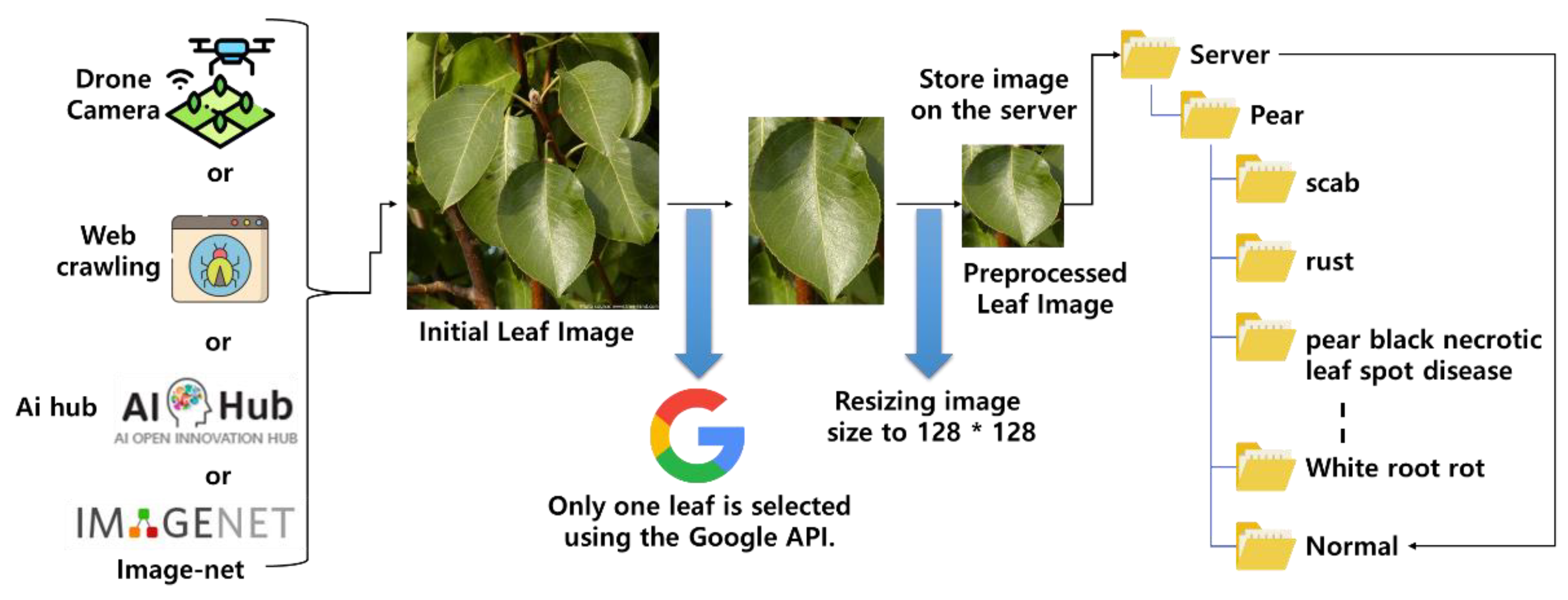
An initial leaf image collected by drone photography and web crawling is not suitable for CNN learning in the CDDM because there are several leaves in one image. Through Google Vision and image resizing, the IPM preprocesses the initial leaf image so that the image has only one leaf, as shown in Figure 4. The IPM selects one leaf image from the initial leaf image and resizes it to 128 × 128, and then stores the preprocessed leaf images in the appropriate folder of the server.
When initial leaf images are collected, they should be precisely classified to judge what kind of crop the leaf comes from and what disease the leaf has. The IPM stores for testing purpose initial leaf images that do not have a disease name among the collected images from drone photography and Google Web, and stores for training purpose images that have a disease name among the collected images from image-net.org and AI hub. The IPM uses Google Vision, which generates 4 coordinate points (upper left, upper right, lower left, and lower right) corresponding to one leaf in an initial leaf image and generates an image of a square leaf by using those points. Algorithm 1 shows the operation process of the IPM.
| Algorithm 1 Image preprocessing of the IPM |
| //Image Preprocessing Algorithm Image Preprocess(Image img){ from google.cloud import vision; Image crop, resize, image; SET hint_params by using image SET image_context by using hint_params SET response by using image and image_context SET hints by using response FOR(n = 1 to hint in enumerate(hints)){ print hint COMPUTE vertices FOR(1 to vertex) print vertices bounds END FOR END FOR IF(size(vertices)==size(image) or hints==null) return null; ELSEIF crop=image.crop(hints); resize=image.resize(crop, 128,128); return resize; END IF } //Image storage algorithm int saveImage(Image img, String imageName, String path, String cropsName, String disease, boolean isTraining){ IF(isTraining) Image preImg = Preprocess(img); IF(preImg != null) saveFile(preImg, path+”\”+cropsName+”\Training\”+disease+”\”+imageName+”.jpg”); return 1; ELSE IF return 0; END IF END IF ELSE saveFile(img, path+”\”+cropsName+”\Test\”+imageName+”.jpg”); return 1; END IF } |
Preprocess() makes an initial leaf image into a preprocessed leaf image. Save Image() stores the preprocessed leaf image in the correct position in the server. Preprocess() works in the following order: First, it receives an initial leaf image and calls Google Vision. Second, it calculates the 4 coordinate points according to the initial leaf image. Third, if the position of the 4 coordinate points is equal to the vertex of the input image, or if there are not 4 coordinate points, Preprocess() returns null. This means the current image cannot be used as training data. Fourth, Preprocess() selects the image according to the 4 coordinate points and resizes the image to 128 × 128. This is the preprocessed leaf image.
If Preprocess() returns the preprocessed leaf image, saveImage() stores it in an appropriate server folder. saveImage() returns 0 or 1; 0 means it did not store the preprocessed leaf image, and 1 means that it did store the image. saveImage() works as follows: First, it receives the initial leaf image and determines whether it is entered as a training image or not. Second, if it is not a training image, it is stored in an image directory for testing; if it is a training image, saveImage() preprocesses it using Preprocess(). Third, when the preprocessing is over, the preprocessed leaf image is stored in an image directory for training if it is assigned to a variable and the variable is not null. If the variable is null, saveImage() concludes that the processed image is not suitable for training and does not store it in the server.
2.3. Design of Crop Disease Diagnosis Module
This paper proposes a crop disease diagnosis module (CDDM) that can diagnose crop diseases by generating CNN models. The CDDM learns the generated CNN models with the leaf images preprocessed by IPM using 30 epochs. The CDDM generates a CNN model for each crop, such as a rice-CNN and tomato-CNN models, etc. A 128 × 128 image is divided into three channels (R, G, B), becoming an input of 128 × 128 × 3. The number of CDDM output nodes is one more than the number of diseases each crop has. For example, if the CDDM generates a tomato-CNN model, the number of output nodes is 12, 11 of them representing 11 diseases that tomatoes can have and one representing healthy tomato. The output value of the CDDM means the probability between 0 and 1 and the node with the highest probability is determined as crop disease.
The CDDM generates a CNN model using 3 convolution and 3 max pooling processes, and a fully connected neural network operations with 3 layers. The convolution and max pooling processes extract the disease characteristics from the leaves, and the neural network calculates a final result, a disease name. The convolution process scans images to extract their characteristics and the output is convolutional feature maps.
In the convolution process, a filter scans images by using an orthogonal matrix of n × n and a stride, a moving unit of a filter. The CDDM uses a 4 × 4 filter; 20 filters are used for the first convolution process, 40 filters for the second, and 60 filters for the third. In the 3 convolution processes, all strides use number 1. The convolution process computes the convolutional feature map using the rectified linear unit (ReLU) function between an image and a filter. The computed convolutional feature map is simplified through max pooling. Max pooling extracts the most characteristic area from image pixels of a regular size and makes it into one pixel.
The CDDM uses a 2 × 2 max pooling technique to simplify the convolutional feature map. Figure 5 shows the convolutional feature map of an image that has undergone 3 convolution and 3 max pooling processes. In Figure 5, the CDDM has the final 16 × 16 convolutional feature map size and 60 channels and changes the 16 × 16 × 60 map to a layer. Figure 6 shows that the 16 × 16 × 60 map in Figure 5 is replaced with the feature map layer and is connected to the buffer layer, which is connected to the output layer. In Figure 6, n−1 represents the number of diseases that can occur in crops.
All the nodes in the fully connected neural network are computed in the same method as the existing multilayer neural network. The CDDM uses softmax for computation as an activation function of the neural network and learns it using the softmax loss function. The result of softmax is between 0 and 1. The CDDM provides the user with the disease name on a node that is greater than 0.75 and stores the output node values in the output table. The CDDM sets values of the output table less than 0.75 to zero, receives an infectious disease name with an output table equal to or greater than 0.75 from a farm server, and stores it in the output table. The CDDM transmits the output table to the CYPM. Equations (1) and (2) represent the softmax function and softmax loss function, respectively.
In Equation (2), represents learning data and the result of neural networks. If the CDDM finishes learning the fully connected neural network by using E, it diagnoses what disease the crop has by recognizing the image and informs the user of the results. Table 1 shows the number of input channels used by the CDDM in the process of generating CNN, the number of filters, the number of output channels, the stride, max pooling unit, and activation function.
2.4. Design of Crop Yield Prediction Module
After the CDDM diagnoses crop disease, the CYPM proposed in this paper predicts crop yield by using information such as crop disease, current weather, and crop status. Figure 7 shows the input and output process of the CYPM based on ANN to accurately predict crop yield, where n, k, p, and j represent the number of diseases that apples, pears, chives, and onions can have, respectively.
The CYPM uses the CDDM outputs (such as disease names and infectious diseases), crop name, remaining date for harvest, temperature, humidity, precipitation, sunshine, ground temperature, atmospheric pressure, evaporation, water pH, water quality, and soil pH in the area. Table 2 shows that the number of input layer nodes in the CYPM is 2n + 13, where n represents the number of diseases that crops can have. Equation (3) represents the set of input nodes in the CYPM.
The output of the CYPM represents the predicted crop yield; that is, the number of output nodes in the CYPM is 1, marked by y. The CYPM uses 5 hidden layers, and each has 20 nodes, as expressed in Equation (4):
In Equation (4), the superscript is the hidden layer number and the subscript is the node number. The nodes in the CYPM are connected to each other, and the weight between the nodes is expressed in Equation (5):
In Equation (5), represents the weight between the first node of the input layer and the first node of the first hidden layer. Next, the CYPM’s learning rate and initial weight should be set to 0.003 and 0.05, respectively. The CYPM learns by using back-propagation and a loss function and activation function. Equation (6) represents the CYPM loss function (mean square error) and Equation (7) the CYPM activation function (ReLU). Since there is one output node of the CYPM, the loss function E can be expressed simply in Equation (6):
E and ReLU have low accuracy when the result of a node is negative, but the calculation speed is fast. Since the CYPM’s input and output values are all positive, Equations (6) and (7) ensure speed without performance degradation. The CYPM computes the error signal using the output node value for back-propagation. The error signal is obtained in Equation (8):
where d is the learning data, y is the output value of the CYPM, and if is calculated, the CYPM computes the error signal of the last hidden layer using . The error signal of the last hidden layer is obtained in Equation (9), and the error signal of the first to the fourth hidden layer in Equation (10):
If the error signals of all layers are computed, the CYPM uses them to modify the weight between nodes. The weight between the last hidden layer and the output layer is modified in Equation (11), between the hidden layers in Equation (12), and between the hidden layer and the input layer in Equation (13). The k of Equation (12) is an integer between 2 and 5.
The learning is terminated when the E (by Equation (6)) of the ANN falls below 0.01. Algorithm 2 shows the LearningCYPM and UsingCYPM functions.
| Algorithm 2 Operation of LearningCYPM and UsingCYPM functions |
| //learning algorithm void LearningCYPM(double dX[][13], double dY[], double a, double w[6][][], Emax, int training_size_n){ SET Initial eSignal[6][], output y, hidden layer node value to 0 and e value to 9999; WHILE (e is greater than Emax) FOR (i= 1 to the number of input layer nodes) y=UsingCYPM(dX[i], w[6][][], 12); END FOR //e computation using loss function e= (dY[i]-y)2; //the computation of error signal eSignal[5][0] = dY[i]-y; FOR(j = 1 to the number of hidden layer nodes) eSignal[4][j] = a*eSignal[5][0]*w[5][j][0]; END FOR FOR(p = 1 to the number of hidden layer) FOR(k = 1 to the number of hidden layer nodes) FOR(j = 1 to the number of hidden layer nodes) eSignal[p][k]=a*eSignal[p+1][j]*w[p+1][k][j]; END FOR END FOR END FOR // weight modification FOR(j = 1 to the number of last hidden layer nodes) w[5][j][0] = w[5][j][0] + a*h[4][j]*eSignal[5][0]; END FOR FOR(p = 4 to 1) FOR(k = 1 to the number of hidden layer nodes) FOR(j = 1 to the number of hidden layer nodes) w[p][j][k] = w[p][j][k] + a*h[p-1][j]*eSignal[p][k] END FOR END FOR END FOR FOR(j = 1 to the number of input layer nodes) FOR(p = 1 to the number of hidden layer nodes) w[0][j][p] = w[0][j][p] + a*x[j]*eSignal[0][p] END FOR END FOR END WHILE } // CYPM computation algorithm double UsingCYPM(double X[], double w[][][]){ SET h[5][size_x+16], NET =0; FOR(p = 1 to the number of hidden layer nodes) FOR(j = 1 to the number of input layer nodes) NET = NET+(x[j]*w[0][j][i]); END FOR h[0][i] = Max(0, NET); NET=0; END FOR FOR(p = 1 to the number of hidden layer) FOR(p = 1 to the number of hidden layer nodes) FOR(j = 1 to the number of hidden layer nodes) NET = NET+(x[j]*w[k][j][i]); END FOR h[k][i] = Max(0, NET); NET=0; END FOR END FOR FOR(j = 1 to the number of hidden layer nodes) NET=h[4][i]*w[5][i][0] END FOR y=Max(0, NET); RETURN y; } |
LearningCYPM in Algorithm 2 shows the process by which the CYPM learns the neural network model using the learning dataset, and UsingCYPM shows the process by which the CYPM returns the result for a specific input. Figure 8 shows the structure of the ANN in the CYPM. The CYPM predicts crop yield per unit area based on weather, crop status, and crop disease information. The learning data are generalized per unit area of the farm. The CYPM uses crop yield data provided by the Korean Statistical Information Service.
3. Results and Discussion
3.1. CDDM Performance Analysis
In this paper, the CNN used for the CDDM is compared with R-CNN and YOLO in operation time and accuracy. We used 5000–20,000 test datasets composed of leaf images and disease names. Thus, the actual number of datasets is equal to the number of actual images used in the experiment. For the experiment, the images of datasets were randomly selected among the images preprocessed in IPM. The number of the randomly selected datasets started at 5000 and were increased by 500.
The experiment was conducted on a PC with 8 GB RAM and 3.40 GHz CPU. Figure 9 shows the accuracy of CNN, R-CNN, and YOLO according to the number of test datasets.
As shown in Figure 9, the CNN has 100% accuracy in processing 5500 datasets, 99.96% for 8000 datasets, 99.79% for 11,000 datasets, 99.96% for 14,000 datasets, 99.68% for 16,000 datasets, 99.6% for 18,000 datasets, and 99.54% for 20,000 datasets. R-CNN has 99% accuracy in processing 5500 datasets, 98.91% for 8000 datasets, 97.99% for 11,000 datasets, and 97.99% for 14,000 datasets. YOLO has 96.98% accuracy in processing 5500 datasets, 96.55% for 8000 datasets, 95.21% for 11,000 sets, 94.21% for 14,000 datasets, 93.18% for 16,000 datasets, 95.22% for 18,000 datasets, and 95.01% for 20,000 datasets. Table 3 shows the number of datasets in which each neural network model failed to diagnose. The number of total datasets in Table 3 represents the number of total datasets used in the experiment, disease name failure means the number of datasets in which each neural network model incorrectly diagnosed the name of the disease, and disease count failure means the number of datasets that incorrectly diagnosed the number of diseases. For example, when the number of datasets in Table 3 is 8000, the number of datasets is six in case the R-CNN misjudged the name of the disease, and the number of datasets is one in case it misjudge the number of diseases.
Therefore, CNN has a maximum accuracy of 100% and a minimum accuracy of 99.54%; R-CNN has a maximum accuracy of 99% and a minimum accuracy of 95.01%; and YOLO has a maximum accuracy of 96.98% and a minimum accuracy of 92.75%.
Here, average accuracy for CNN is 99.6%, for R-CNN is 96.1%, and for YOLO is 94.2%. CNN’s average accuracy is about 3.5% higher than R-CNN’s and about 5.4% higher than YOLO’s. Smart farms, where many crops are grown, should prefer CNN to the other models to accurately diagnose crop diseases.
Figure 10 shows the operation time of CNN, R-CNN, and YOLO according to the number of test datasets. CNN has an operation time of 172 s in processing 5500 datasets, 211 s for 8000, 243 s for 11,000, 265 s for 14,000, 276 s for 16,000, 286 s for 18,000, and 293 s for 20,000. R-CNN has an operation time of 102 s in processing 5500 datasets, 134 s for 8000, 190 s for 11,000, 231 s for 14,000, 251 s for 16,000, 269 s for 18,000, and 286 s for 20,000. YOLO has an operation time of 65 s in processing 5500 datasets, 72 s for 8000, 119 s for 11,000, 178 s for 14,000, 212 s for 16,000, 235 s for 18,000, and 255 s for 20,000. CNN takes an average of 232.5 s to process datasets 5500 to 20,000 datasets, R-CNN takes 195.5 s, and YOLO takes 160 s. CNN takes about 37 s more than R-CNN and about 72 s more than YOLO in operation time. According to linear regression, the slope of CNN operation time is 8.1032E-3, R-CNN is 1.5642E0, and YOLO is 1.0934E0, i.e., the operation time of R-CNN and YOLO is greater than that of CNN as the amount of data grows. Therefore, CNN has longer operation time and higher accuracy than R-CNN and YOLO. Because the CDDM has to consider accuracy more than operation time for accurate yield prediction, it selects the CNN.
3.2. CYPM Performance Analysis
In this section, three experiments were conducted to analyze the performance of the CYPM. First, five-fold cross-validation was conducted using the training datasets from the CYPM. Five-fold cross-validation is an algorithm that divides the images preprocessed in the IPM into training datasets and test (validation) datasets and cross-validates the neural network by dividing the training datasets evenly into k validation folds [27]. The CYPM uses 90% of the images preprocessed in the IPM as training datasets, and measures cross-validation accuracy by increasing the number of validation folds from 1 to 50. Second, the ReLU is used in the CYPM as activation function and compared with Sigmoid and Step functions for performance analysis. Third, a predicted yield is measured when a disease is used as input to the CYPM to check its effect on yield, and a predicted error rate when it is not. The experimental environment is the same as that of the CDDM.
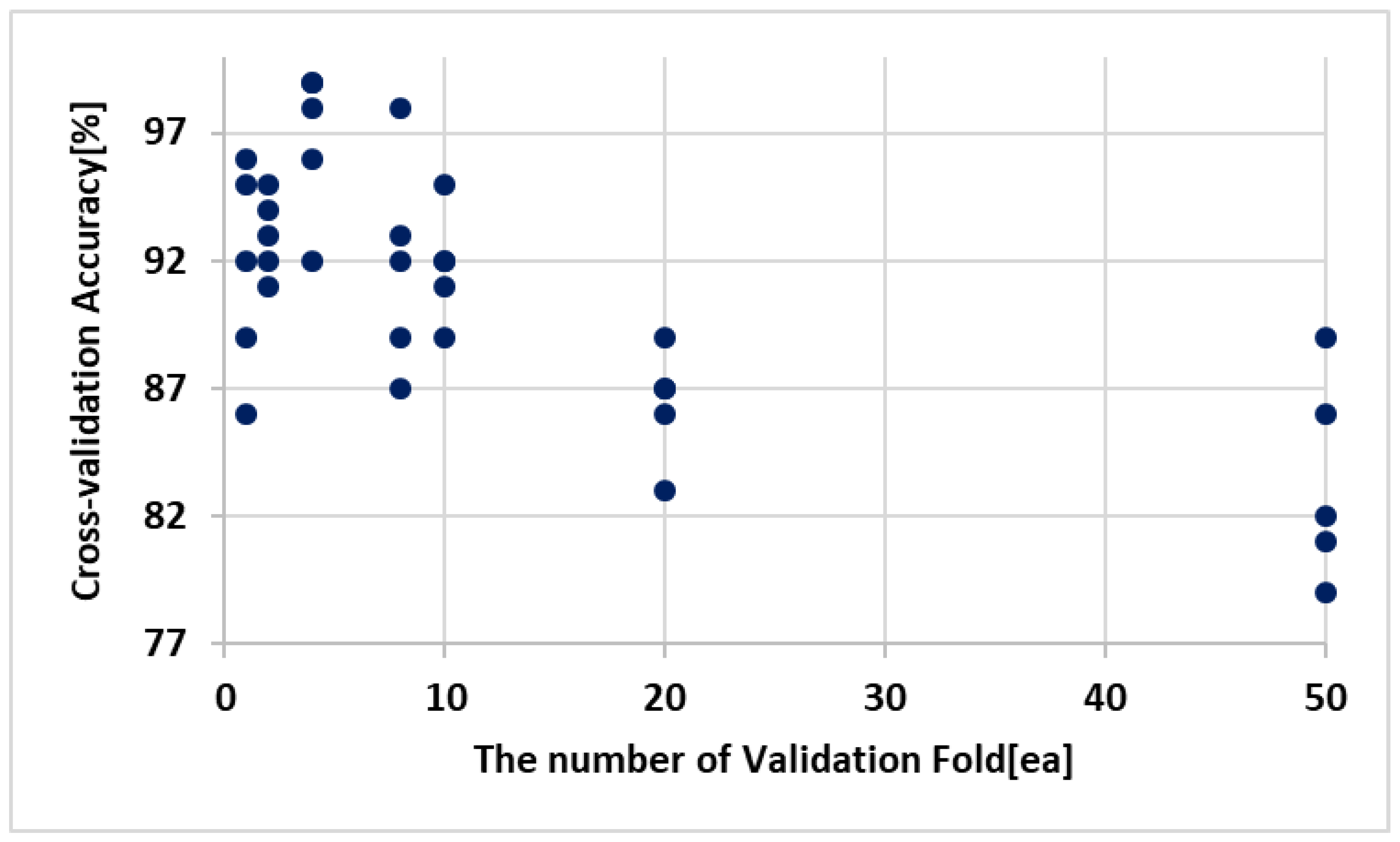
As shown in Figure 11, the number of validation folds used for five-fold cross-validation is from 1 to 50. The average cross-validation accuracy is 91.6% with 1 fold, 93% with 2, 96.8% with 4, 91.8% with 8, 86.4% with 20, and 83.4% with 50. Therefore, the CYPM should optimize its learning rate (hyperparameter) using four validation folds.
The accuracy of ReLU shown in Figure 12 is 95.9% for 5500 test datasets, 99.9% for 8000, 98.68% for 11,000, 97.14% for 14,000, 96.21% for 16,000, 95.92% for 18,000, and 95.58% for 20,000. The accuracy of the Sigmoid function is 100% for 5500 test datasets, 99.9% for 8000, 98.68% for 11,000, 97.14% for 14,000, 96.21% for 16,000, 95.92% for 18,000, and 95.58% for 20,000. The accuracy of the Step function is 96.85% for 5500 test datasets, 96.12% for 8000, 94.97% for 11,000, 92.28% for 14,000, 90.14% for 16,000, 88.12% for 18,000, and 86.01% for 20,000. Since all inputs of the CYPM and the initial weight values are positive, the disadvantage that ReLU has lower accuracy when the node result of a neural network is negative disappears.
According to linear regression, the slope of accuracy with is −3.641 × 10⁻⁴ with ReLU, −4.0710 × 10⁻⁴ with Sigmoid, and −7.4534 × 10⁻⁴ with Step. Therefore, since the accuracy slope is the lowest when using ReLU, ReLU is more accurate than the other two activation functions as the amount of test data increases.
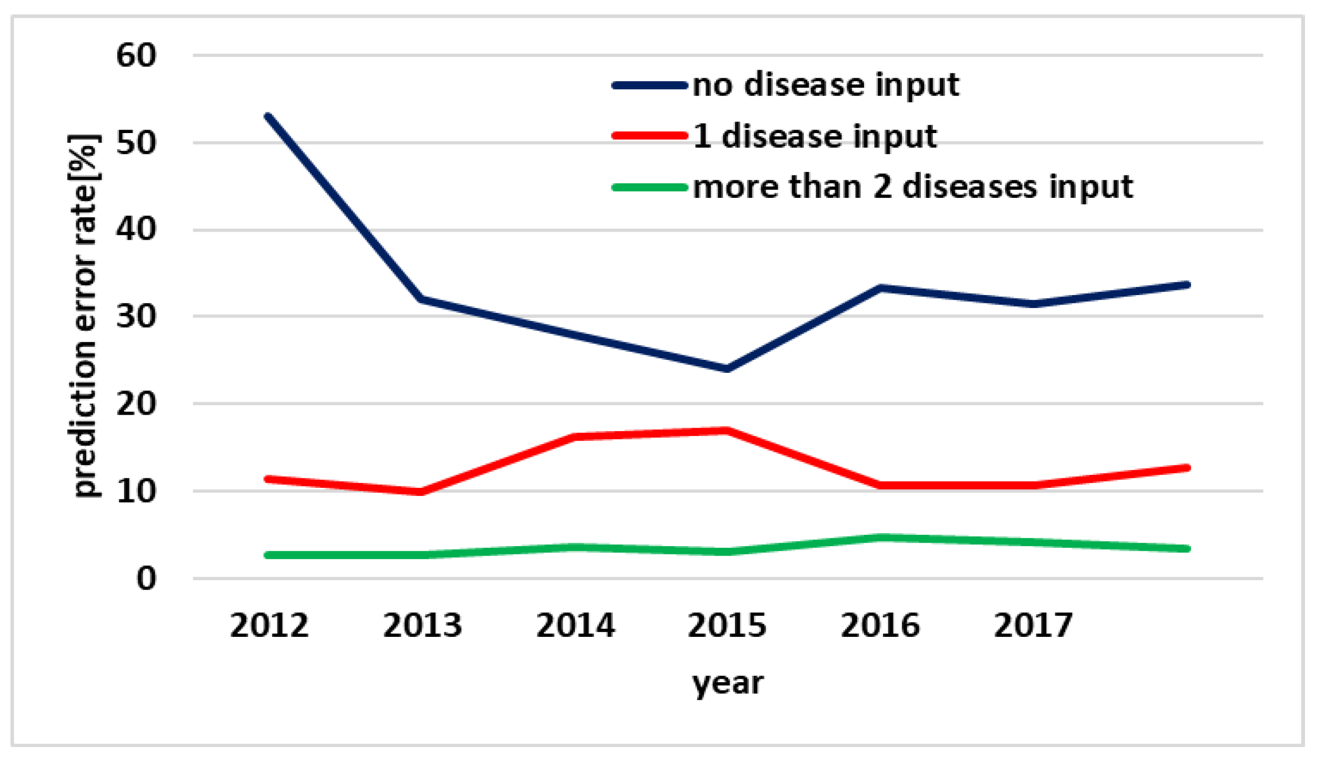
Figure 13 shows the actual yield of pears and the error rate of predicted yield for the CYPM during 2012–2017. The error rate was computed using mean absolute percentage error, represented by Equation (14):
In Equation (14), E is the computed error rate, d is the actual yield, and y is the predicted yield. The CYPM estimates yield by using the same leaf images and environmental information on 10 August each year. The average error rate for predicted yield is 33.637% when the CYPM does not use a disease as input, and for predicted yield is 10.624% when the CYPM uses only one disease. Finally, when the CYPM uses two or more diseases as input, the error rate for predicted yield is 3.476%.
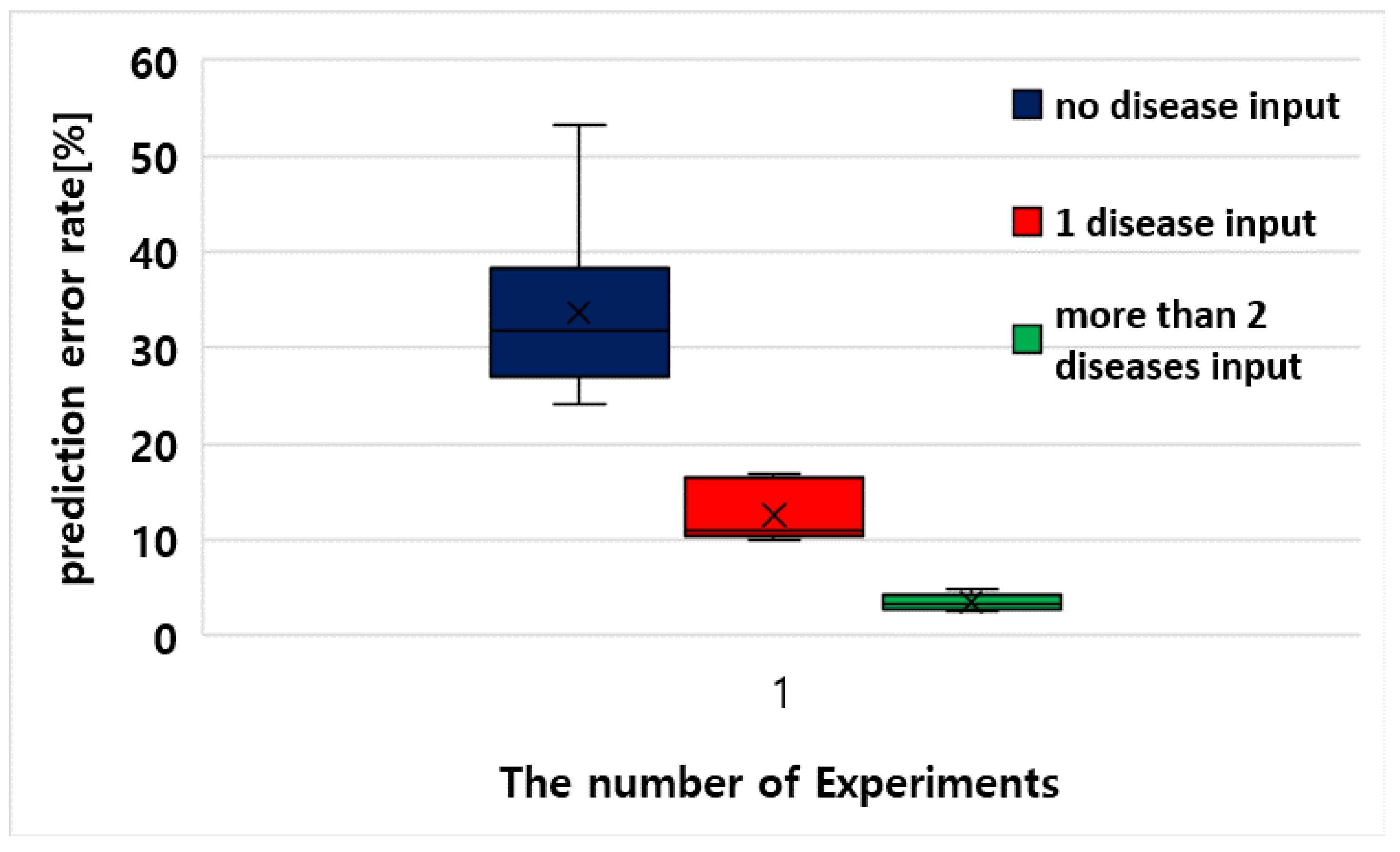
If the CYPM uses two or more diseases as input to predict the yield of pears, its error rate is about 30% lower than when a disease is not used as input and about 7% lower than when only one disease is used. Figure 14 shows the confidence limits of experimental results in a boxplot. Therefore, the CYPM should take into account various diseases that may occur in the crop to accurately predict the yield.
Figure 15 shows the estimated yield during 2012–2017 when the CYPM takes into account disease epidemics and when it does not. When the CYPM does not take them into account, the yield is predicted to be 316 tons less than the yield in 2012, 908 tons in 2013, 716 tons in 2014, 669 tons in 2015, 671 tons in 2016, and 834 tons in 2017. The CYPM predicts an average yield of 687.16 tons when considering disease epidemics. When the CYPM predicts yield by considering disease epidemics, farmers will realize the severity of the infectious diseases more quickly and try to fight against the epidemic. Figure 16 shows the confidence limits of experimental results in a boxplot.
4. Conclusions
This paper proposes a self-predictable crop yield platform (SCYP) based on crop diseases using deep learning to diagnose crop diseases through leaf images of crops and predict a farm’s annual yield using the diagnosis result and environmental information. The SCYP consists of a crop disease diagnosis module (CDDM) that uses crop photographs and a crop yield prediction module (CYPM) that uses the CDDM’s disease information and environmental information. Four experiments were conducted to verify the efficiency of the SCYP. In the first experiment, the accuracy of the CNN used by the CDDM was about 3.5% higher than that of R-CNN and 5.4% higher than that of YOLO. In the second experiment, the CNN’s operation time was about 195.5 s longer than that of R-CNN and 160 s longer than that of YOLO. The CDDM uses CNN, which is more accurate for disease management even if it is slower than R-CNN and YOLO. In the third experiment, the ReLU used by the CYPM had an accuracy of about 1% higher than the Sigmoid function and about 10% higher than the Step function. In the last experiment, the CYPM predicted yields about 34% more accurately when using multiple diseases than when not using them. Therefore, the SCYP can predict farm yields more accurately than traditional methods.
The SCYP has the following advantages over existing research methods. First, unlike previous studies that diagnosed only one disease, it can diagnose a number of diseases that are more likely to occur with higher accuracy. Second, by using disease and environmental information on crops, the SCYP can predict crop yields accurately. In this paper, past harvest data were used to diagnose crop diseases and predict crops, but in future studies, crops should be diagnosed and yields predicted on real farms. Also, ways to improve operation time while maintaining the accuracy of the CNN used in the CDDM should be studied.
Author Contributions
Conceptualization, B.L.; methodology, Y.J.; software, S.S.; validation, B.L.; formal analysis, S.L.; writing—original draft preparation, Y.J. and S.S.; writing—review and editing, B.L.; supervision, B.L.; project administration, B.L. and S.L.; funding acquisition, S.L.
Funding
This work was supported by the Regional New Project Leader Training Project through the Ministry of Education and National Research Foundation of Korea (NRF-2016H1D5A1909417).
Conflicts of Interest
The authors declare no conflicts of interest.
References
- Use Case: Precision Agriculture, the Internet of Things, and Big Data Management. Available online: https://helioswire.com/case-study-precision-agriculture-the-internet-of-things-and-big-data-management/ (accessed on 18 April 2019).
- Precision Ag & Big Data Learning. Available online: https://www.precisionag.com/systems-management/data/precision-ag-big-data-learning/ (accessed on 20 April 2019).
- Plant Village: A Deep-Learning App Diagnoses Crop Diseases. Available online: https://actu.epfl.ch/news/plantvillage-a-deep-learning-app-diagnoses-crop-di/ (accessed on 16 April 2019).
- Jirapond, M.; Nathaphon, B.; Siriwan, K.; Narongsak, L.; Apirat, W.; Pichetwut, N. IoT and agriculture data analysis for smart farm. Comput. Electron. Agric. 2019, 156, 467–474. [Google Scholar]
- Chae, C.-J.; Cho, H.-J. Enhanced secure device authentication algorithm in P2P-based smart farm system. Peer-To-Peer Netw. Appl. 2018, 11, 1230–1239. [Google Scholar] [CrossRef]
- Hwang, S.I.; Joo, J.-M.; Joo, S.-Y. ICT-based smart farm factory systems through the case of hydroponic ginseng plant factory. J. Korean Inst. Commun. Inf. Sci. 2015, 40, 780–790. [Google Scholar]
- Jo, H.-K.; Choi, H.-H.; Kim, D.-S.; Lee, J.-M. Design and implementation of smart farm wireless network: LoRa and IEEE 802.11 wireless backhaul network. J. Korean Inst. Commun. Inf. Sci. 2018, 43, 850–862. [Google Scholar] [CrossRef]
- Gan, H.; Lee, W.S. Development of a navigation system for a smart farm. IFAC-PapersOnLine 2018, 51, 1–4. [Google Scholar] [CrossRef]
- Kim, J.M.; Moon, S.J.; Hwang, D.-Y. A Study on greenhouse smart farm system based on wireless sensor. Adv. Sci. Lett. 2018, 24, 2041–2045. [Google Scholar] [CrossRef]
- Choi, W.H.; Jie, M.S. Study on the development of wireless sensor network using smart farm system. J. Korea Entertain. Ind. Assoc. 2014, 8, 387–393. [Google Scholar] [CrossRef]
- Liu, B.L.; Yuan, M.H.; Chen, G.R.; Peng, J. The design and simulation of a smart farm system based on ultra-narrow band communication. Science 2013, 427, 1398–1401. [Google Scholar]
- Suk, C.M. Development of serious game system for cultivating using smart farm technology. KSCG 2016, 29, 35–41. [Google Scholar]
- Jeong, Y.N.; Son, S.; Lee, S.S.; Lee, B.K. A total crop-diagnosis platform based on deep learning models in a natural nutrient environment. Appl. Sci. 2018, 8, 1992. [Google Scholar] [CrossRef]
- Feng, S.J.; Gang, W.; Yong, W. The dynamic model prediction study of the forest disease, insect pest and rat based on BP neural networks. J. Agric. Sci. 2012, 4, 221–224. [Google Scholar]
- Alves, D.P.; Tomaz, R.S.; Laurindo, B.S.; Laurindo, R.D.S.; Silva, F.F.E.; Cruz, C.D.; Nick, C.; da Silva, D.J.H. Artificial neural network for prediction of the area under the disease progress curve of tomato late blight. Sci. Agric. 2017, 74, 51–59. [Google Scholar] [CrossRef] [Green Version]
- Igarashi, W.T.; de França, J.A.; Silva, M.A.; de Igarashi, S.; Saab, O.J.G.A. Application of prediction models of asian soybean rust in two crop seasons, in Londrina, Pr. Semina Ciências Agrárias 2016, 37, 2881–2890. [Google Scholar] [CrossRef]
- Etebu, E.; Osborn, A.M. Molecular prediction of pea footrot disease. Asian J. Agric. Sci. 2011, 3, 417–426. [Google Scholar]
- Goldstein, A.; Fink, L.; Meitin, A.; Bohadana, S.; Lutenberg, O.; Ravid, G. Applying machine learning on sensor data for irrigation recommendations: Revealing the agronomist’s tacit knowledge. Precis. Agric. 2017, 19, 421–444. [Google Scholar] [CrossRef]
- Tanaka, K. A java framework for developing a plant growth and disease prediction model. Agric. Inf. Res. 2006, 15, 183–193. [Google Scholar]
- Amar, D.; Vizel, A.; Levy, C.; Shamir, R. ADEPTUS: A discovery tool for disease prediction, enrichment and network analysis based on profiles from many diseases. Bioinformatics 2018, 34, 1959–1961. [Google Scholar] [CrossRef]
- Okonya, J.S.; Ocimati, W.; Nduwayezu, A.; Kantungeko, D.; Niko, N.; Blomme, G.; Legg, J.P.; Kroschel, J. Farmer reported pest and disease impacts on root, tuber, and banana crops and livelihoods in Rwanda and Burundi. Sustainability 2019, 11, 1592. [Google Scholar] [CrossRef]
- Abdipour, M.; Younessi-Hmazekhanlu, M.; RezaRamazani, S.H.; Omidi, A.H. Artificial neural networks and multiple linear regression as potential methods for modeling seed yield of safflower (Carthamus tinctorius L.). Ind. Crops Prod. 2019, 127, 185–194. [Google Scholar] [CrossRef]
- Niedbała, G. Application of artificial neural networks for multi-criteria yield prediction of winter rapeseed. Sustainability 2019, 11, 533. [Google Scholar] [CrossRef]
- Kerkech, M.; Hafiane, A.; Canals, R. Deep leaning approach with colorimetric spaces and vegetation indices for vine diseases detection in UAV images. Comput. Electron. Agric. 2018, 155, 237–243. [Google Scholar] [CrossRef]
- Barbedo, J.G.A. Plant disease identification from individual lesions and spots using deep learning. Biosyst. Eng. 2019, 180, 96–107. [Google Scholar] [CrossRef]
- Gabryel, M.; Damaševičius, R. The image classification with different types of image features. Int. Conf. Artif. Intell. Soft Comput. 2017, 10245, 497–506. [Google Scholar]
- Improve Your Model Performance Using Cross Validation (in Python and R). Available online: https://www.analyticsvidhya.com/blog/2018/05/improve-model-performance-cross-validation-in-python-r/ (accessed on 10 June 2019).
Figure 1.
Structure of smart farm.

Figure 2.
Structure of artificial neural network (ANN).

Figure 3.
Structure of the self-predictable crop yield platform (SCYP).

Figure 4.
Image preprocessing.

Figure 5.
Convolution and max pooling process of the crop disease diagnosis module (CDDM).

Figure 6.
Process of changing a convolutional feature map to a neural network model.

Figure 7.
Input and output process of the crop yield prediction module (CYPM).

Figure 8.
ANN of the CYPM.

Figure 9.
Accuracy of convolutional neural network (CNN) compared with region-CNN (R-CNN) and you only look once (YOLO) models.
Figure 9.
Accuracy of convolutional neural network (CNN) compared with region-CNN (R-CNN) and you only look once (YOLO) models.

Figure 10.
Operation time of CNN compared with R-CNN and YOLO models.

Figure 11.
Cross-validation accuracy of the CYPM.

Figure 12.
Accuracy of the CYPM by activation function.

Figure 13.
Error rate between actual and predicted yield of pears from 2012 to 2017.

Figure 14.
Boxplot of error rate between actual and predicted yield.

Figure 15.
CYPM predicted yield from 2012 to 2017.

Figure 16.
Boxplot of predicted yield.


Table 1.
Information of the CDDM model.
| Layer | Input Channel | Filter | Output Channel | Stride | Max Pooling | Activation Function |
|---|---|---|---|---|---|---|
| Convolution layer 1 | 3 | (4, 4) | 20 | 1 | – | ReLU |
| Max pooling layer 1 | 20 | – | 20 | 2 | (2, 2) | – |
| Convolution layer 2 | 20 | (4, 4) | 40 | 1 | – | ReLU |
| Max pooling layer 2 | 40 | – | 40 | 2 | (2, 2) | – |
| Convolution layer 3 | 40 | (4, 4) | 60 | 1 | 1 | ReLU |
| Max pooling layer 3 | 60 | – | 60 | 2 | (2, 2) | – |
| Flatten | – | – | – | - | – | – |
| Fully connected layer | – | – | – | - | – | Softmax |
Table 2.
Input nodes of the CYPM.
| Input Node | Description | Source |
|---|---|---|
| Disease 1 | CDDM | |
| Disease 1′ infectious | ||
| Disease 2 | ||
| Disease 2′ infectious | ||
| Disease 3 | ||
| Disease 3′ infectious | ||
| … | … | |
| Normal | ||
| Precipitation | meteorologicaladministration | |
| Humidity | ||
| Sunshine | ||
| Temperature | ||
| Ground temperature | ||
| Evaporation | ||
| Atmospheric pressure | ||
| Crop name | server | |
| Date remaining (daily) to harvest | ||
| Water pH | ||
| Water quality | ||
| Soil pH |
Table 3.
The number of datasets that the CDDM failed to diagnose.
| The Number of Total Datasets | R-CNN | YOLO | CNN | |||
|---|---|---|---|---|---|---|
| Disease Name Failure | Disease Count Failure | Disease Name Failure | Disease Count Failure | Disease Name Failure | Disease Count Failure | |
| 5500 | 0 | 0 | 1 | 0 | 0 | 0 |
| 6000 | 9 | 1 | 1 | 0 | 0 | 0 |
| 6500 | 6 | 0 | 2 | 1 | 2 | 1 |
| 8000 | 6 | 1 | 31 | 5 | 2 | 1 |
| 8500 | 15 | 1 | 35 | 7 | 3 | 2 |
| 10,000 | 29 | 2 | 96 | 10 | 10 | 3 |
| 10,500 | 34 | 2 | 101 | 12 | 11 | 3 |
| 12,000 | 115 | 10 | 306 | 28 | 21 | 8 |
| 12,500 | 152 | 17 | 344 | 29 | 22 | 9 |
| 14,000 | 244 | 21 | 478 | 53 | 33 | 10 |
| 14,500 | 223 | 25 | 528 | 51 | 30 | 8 |
| 16,000 | 371 | 39 | 682 | 89 | 39 | 12 |
| 16,500 | 426 | 34 | 691 | 98 | 46 | 8 |
| 18,000 | 599 | 81 | 802 | 100 | 52 | 9 |
| 18,500 | 622 | 75 | 841 | 93 | 64 | 8 |
| 20,000 | 712 | 86 | 930 | 120 | 82 | 10 |
© 2019 by the authors. Licensee MDPI, Basel, Switzerland. This article is an open access article distributed under the terms and conditions of the Creative Commons Attribution (CC BY) license (http://creativecommons.org/licenses/by/4.0/).
Share and Cite
MDPI and ACS Style
Lee, S.; Jeong, Y.; Son, S.; Lee, B. A Self-Predictable Crop Yield Platform (SCYP) Based On Crop Diseases Using Deep Learning. Sustainability 2019, 11, 3637. https://doi.org/10.3390/su11133637
AMA Style
Lee S, Jeong Y, Son S, Lee B. A Self-Predictable Crop Yield Platform (SCYP) Based On Crop Diseases Using Deep Learning. Sustainability. 2019; 11(13):3637. https://doi.org/10.3390/su11133637
Chicago/Turabian StyleLee, SangSik, YiNa Jeong, SuRak Son, and ByungKwan Lee. 2019. "A Self-Predictable Crop Yield Platform (SCYP) Based On Crop Diseases Using Deep Learning" Sustainability 11, no. 13: 3637. https://doi.org/10.3390/su11133637
Note that from the first issue of 2016, this journal uses article numbers instead of page numbers. See further details here.