The Role of Cultural Landscapes in the Delivery of Provisioning Ecosystem Services in Protected Areas


1
Department of Biology and Geology, University of Almería, 04120 Almería, Spain
2
Department of Applied Mathematics, Rey Juan Carlos University, 28933 Madrid, Spain
*
Author to whom correspondence should be addressed.
†
These authors contributed equally to this work.
Sustainability 2019, 11(9), 2471; https://doi.org/10.3390/su11092471
Submission received: 27 March 2019
/
Revised: 20 April 2019
/
Accepted: 23 April 2019
/
Published: 26 April 2019
(This article belongs to the Special Issue Agriculture, Landscape, Ecosystem Services and Biodiversity: New Challenges for Sustainable Development)
Abstract
:The aim of this paper is to assess and highlight the significance of cultural landscapes in protected areas, considering both biodiversity and the delivery of provisioning ecosystem services. In order to do that, we analyzed 26 protected areas in Andalusia (Spain), all of them Natural or National Parks, regarding some of their ecosystem services (agriculture, livestock grazing, microclimate regulation, environmental education and tourism) and diversity of the four terrestrial vertebrate classes: amphibians, reptiles, mammals, and birds. A cluster analysis was also run in order to group the 26 protected areas according to their dominant landscape. The results show that protected areas dominated by dehesa (a heterogeneous system containing different states of ecological maturity), or having strong presence of olive groves, present a larger area of delivery of provisioning ecosystem services, on average. These cultural landscapes play an essential role not only for biodiversity conservation but also as providers of provisioning ecosystem services.
1. Introduction
Biodiversity conservation has been the cornerstone of conservation strategies in protected areas (PAs). As an example, the Convention on Biological Diversity [1] considers PAs as “geographically defined areas, which are designated or regulated and managed to achieve specific conservation objectives (article 2), focused on biological diversity (article 8 a, b)”. In this sense, until the 1990s to mid 2000s, the conservation values considered in PAs were intrinsic values of ecosystems, biodiversity and cultural values [2]. The main purpose of protected areas was to protect emblematic and flashy species. With the landscape approach in conservation, ecological processes (functions and ecological integrity) were also considered. Currently, the conservation values of PAs are the intrinsic and instrumental values of ecosystems and biodiversity [2]. This approach was taken into account in the definition of PAs by the International Union for Conservation of Nature (IUCN) [3] as “clearly defined geographical spaces, recognized, dedicated and managed, through legal or other effective means, to achieve the long-term conservation of nature with associated ecosystem services and cultural values”.
This new approach considers multifunctional landscapes, resilience, and adaptive management as key concepts in PA conservation, and it agrees with the new conservation science [4] that emphasizes that future conservation efforts will increasingly be focused on areas that have been and will likely continue to be affected by human activities. For this reason, conservation should address human well-being [5]. Therefore, this approach involves recognizing that society and biophysical factors are strongly linked across multiple scales, and they are considered a social-ecological system [6]. In this way, not only ecological but also the social processes are considered in conservation decisions [7].
Cultural landscapes are the result of an intricate relationship between social and ecological systems [8]. They have taken centuries to reach their current configuration, reflecting a mutual adaptation of abiotic, biotic and cultural factors [9], and are considered complex adaptive social-ecological systems [10,11]. These landscapes, rarely uniform or monotonous, are frequently a mosaic with different degrees of ecological maturity [12] and the socioeconomic activities are strongly related to these landscapes [13,14]. Traditional agriculture is part of these landscapes, with extensive and semi-extensive land uses. This agriculture is adapted to natural production cycles and is characterized by its efficiency in the use of energy and nutrients [13]. In Andalusia, the dehesa system is an example of cultural landscapes. These human-shaped ecosystems have a high heterogeneity due to its changing composition and tree cover density [15], mixed with pastures, shrubs and the presence of important livestock grazing. As a whole, dehesa systems are archetypes of High Nature Value farmland [16]. Their ecological value is a result of their contribution to biodiversity at the landscape level, their dynamic character and their role as a repository of genetic resources [17]. These systems are threatened by intensification and abandonment process [14,18,19].
Natural protected areas have played an important role in the conservation of these systems not only by the cultural heritage or biodiversity but also for the large presence of other traditional agricultural systems, such as extensive agriculture of olive groves, and other traditional crops. From a holistic view, these systems play an essential role in the human food supply. The Common Agriculture Policy (CAP) ensures Europe’s food security. The purposes and benefits of the CAP are related to food production, rural community development and environmentally sustainable farming. In this sense, the new post-2020 CAP proposes nine objectives, which cover specific concerns about the environment and climate. Cultural landscapes inside PAs should play an important role in the development of these objectives. However, sometimes these kinds of PAs are considered as the ‘ugly ducklings’ of the protected areas, in the sense that they do not receive the same attention as those with greater tradition in the conservation of emblematic or endangered species. The aim of this paper is to assess and highlight the significance of these systems considering both the biodiversity and the delivery of provisioning ecosystem services.
2. Methodology
2.1. Study Area
The study area is Andalusia, a region located in southern Spain, which occupies an area of 87,000 km and whose latitude and longitude is between 36 N–3844 N and 350 W–034 E. The main mountain ranges are the Sierra Morena mountain range in the North and the Baetic Systems in the South (comprising the Prebaetic, Subbaetic and Penibaetic Systems), which are separated by the Baetic Depression, the lowest territory in Andalusia. The flattest areas correspond to the Littoral and the Baetic depression and the steepest ones to the Baetic Systems. Therefore, Andalusia is divided into 4 main geomorphological units: the Baetic Depression, the Sierra Morena mountain range, the Baetic Systems, and the Littoral. There are 243 protected areas in the study area, with 24 being Natural Parks and 2 being National Parks (Figure 1). In this work, only Natural and National Parks are analyzed and will be referred to as protected areas (PAs). The smallest PA is called La Breña y Marismas de Barbate, with an area of 50.77 km, of which 39.25 km are emerged lands. The largest PA corresponds to Sierras de Cazorla, Segura y las Villas, with an area of 2097.63 km.
The Baetic Depression has fertile soils and high agricultural production, mainly comprising rain-fed herbaceous crops in the low-lying plain and irrigated herbaceous crops along the Guadalquivir River. The Sierra Morena mountain range is mainly covered by rain-fed crops and dehesa, a heterogeneous system containing different states of ecological maturity, with shepherding being the principal economic activity. This unit has six designated protected areas. The Baetic Systems have the highest elevation and steepness in the study area and are mainly covered by natural vegetation and, secondarily, by extensive woody crops. There are 14 protected areas in this geomorphological unit, including the Sierra Nevada National Park. Finally, the Littoral is densely populated, has relatively high temperatures and is covered by natural vegetation and artificial areas, including most greenhouses. There are six protected areas in the Littoral, including the Doñana National Park, which is the largest reserve of birds in Europe.
2.2. Data Collection
Data of the presence of terrestrial vertebrates were obtained from the Spanish Inventory of Terrestrial Species (www.miteco.gob.es/es/biodiversidad). This dataset provides information about the presence of species in a grid with a cell width of 10 km. There are 386 terrestrial vertebrate species in the study area: 259 birds, 62 mammals, 43 reptiles and 22 amphibians.
The information describing the land-use of Andalusia was obtained from the Land use and vegetation cover map of Andalusia of 2011 (at scale 1:10,000) (www.juntadeandalucia.es/medioambiente/site/rediam/), which is based on the Land Occupation Information System of Spain (SIOSE). In particular, the level of detail used was “inspection”, containing 16 different types. Some of these land-use types were aggregated into new broader categories, obtaining 11 land-use variables. The correspondence between the SIOSE-based cartography and the aggregated land-uses can be seen in Table 1. From now on, the aggregated land-use variables will be referred to as (with ). The aforementioned grid was used to calculate the proportion of within each cell. The proportion of each within each protected area was also computed.
Finally, the landscape cartography of Andalusia was obtained from the Landscape Map of Andalusia of 2005 (at scale 1:100,000) (www.juntadeandalucia.es/medioambiente/site/rediam). This cartography reflects the different categories of morphology and land-use of Andalusia and matches the landscape types considered in the Dobris report [20] for the assessment of the state of the environment in Europe. Therefore, this cartography is closely linked to the Land use and vegetation cover map of Andalusia. The landscape cartography of Andalusia provides the spatial distribution of 34 landscape units (LSUs, Table 2). The proportion of each LSU within each PA was computed for further analysis.
2.3. Data Preparation
This section aims at describing how the ecosystem service variables and the diversity of terrestrial species variable are constructed from the raw datasets.
2.3.1. Ecosystem Service Variables
Ecosystem services (ES) are defined as the benefits that human population obtains from ecosystems [21]. Typically, these services are grouped under 3 general categories: regulating, provisioning and cultural services [21]. In this paper we focus on 5 ES: 2 provisioning (agriculture and livestock grazing), 2 cultural (tourism and environmental education) and 1 regulating (microclimate regulation).
Eight experts (researchers and academics) from the University of Almería, Universidad Complutense de Madrid and Universidad Autónoma de Madrid assessed whether a particular generates a particular ES (1) or not (0). We consider that a land-use generates an ES if at least 80% of the experts agreed on that. An indicator, , was constructed for each pair {, }, so that it can take 2 possible values: 1 (if generates ) or 0 (if not). The set of indicators can be arranged in a matrix, as shown by .
Note that the relationship - is not measured as a quantitative magnitude but as qualitative, i.e., we do not know the amount of produced by each L, we only know if that is produced or not. For instance, pine forests provide tourism services. However, the degree of such relationship is uncertain. Moreover, only some specific features of a land-use might deliver the ES, instead of the entire land-use. Therefore, more detailed results would be obtained if the land-use categories were disaggregated into more specific ones. However, we make no distinction among the different features that compose a specific land-use, but on the contrary they are treated as a whole, for the sake of simplicity.
Once we know which land-use generates which ES, a quantification of the proportion of cell k that generates the can be obtained. Since variables are defined as a proportion, we can compute the scalar product of the land-use matrix, , with each row of matrix , obtaining a vector , whose elements, , are the sum of the products of the elements of row k of matrix and the elements of .
Therefore, represents the proportion of cell that generates the (with ) regarding the distribution of (), with being the proportion of occupation of land use j in cell k. Each cell in the map can be colored across a gradual red to dark green color ramp, where values (≈0) are represented with the red color and high values (≈1) with dark green.
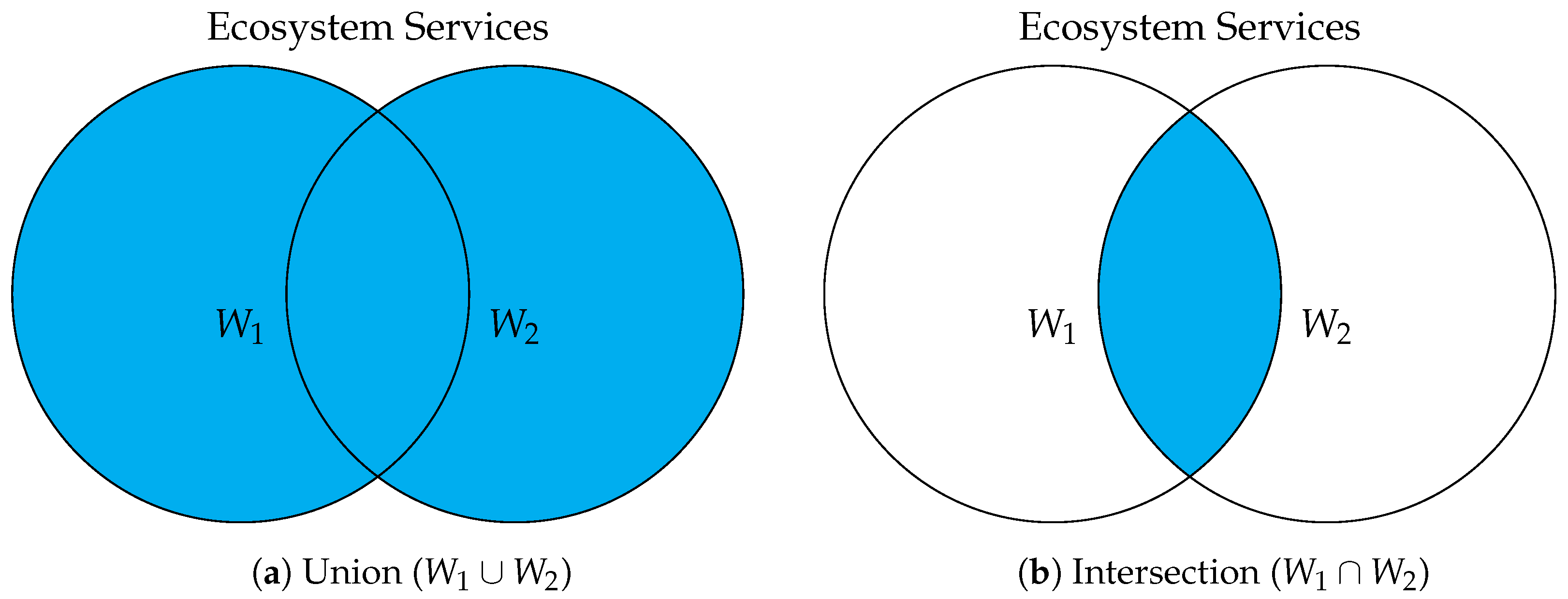
On the other hand, the proportion of the 3 broad ES categories (provisioning, regulating and cultural) within each cell can also be computed in the same manner as explained before, obtaining variables (with ). As variables represent a proportion, i.e., range from 0 to 1, they can also be interpreted as the probability of finding the land-uses that generate the ecosystem service in a cell. Therefore, variables can be interpreted as the union of the variables that belong to category c; for instance, the probability of finding or or both in a cell. Note that since several ecosystem services can overlap, i.e., they are not mutually exclusive. On the contrary, , where is the intersection of the that belong to category c. Figure 2 graphically shows the union and intersection of 2 ecosystem services through Venn diagrams.
2.3.2. Diversity of Terrestrial Vertebrates
The presence of species dataset was used to compute the richness of the 4 terrestrial vertebrate taxonomic classes: amphibians, reptiles, mammals, and birds. The species richness is measured as the number of species (of each class) present in each cell. Shannon’s entropy H can be used as a measure of diversity. In this regard, this index was computed to reflect how many different classes of animals coexist in each cell and how even their relative abundances are. Shannon’s index H is defined as [22]
where is the proportion of species belonging to taxonomic class i and R the total number of classes.
H ranges from 0 to , so that if all the species belong to the same class, . On the other hand, if the proportional abundances of the classes are equal, . The base 2 logarithm was used to compute H. Since 4 classes are being considered in this paper, H ranges from 0 to 2 bits. Each cell in the map can be colored across a gradual red to dark green color ramp, where low values (≈0) are represented with the red color and high values (≈2) with dark green.
2.4. Description of Protected Areas Based on Ecosystem Service and Diversity Variables
The 26 PAs were described in terms of ecosystem service () and diversity (H) variables, which were obtained as explained in Section 2.3. Note that the use of the grid allows obtaining ES maps for the entire study area. However, when focusing on specific regions, such as the protected areas, more accurate variables can be obtained if the raw land-use values are given at the PA scale instead, so that matrix would have the form
with the remainder of the methodology staying the same. Unlike land-uses, the species richness can only be obtained at the grid scale, so that the average value of H within each PA has to be computed. Regarding interpretation, the obtained ecosystem service variables can be understood as the proportion of the PA that generates a given in relation to its total area. For instance, if variable takes the value 0.5 in a PA, then 50% of the PA generates the service.
On the other hand, a value for each ES category (provisioning, regulating and cultural) was obtained as the union of the variables belonging to the c-th ES category, as
where is the union of the variables belonging to the c-th ES category and the intersection of the variables belonging to the c-th ES category. For instance, the union of the provisioning ES is
The obtained variables also range from 0 to 1. These variables can be plotted on different maps so that each PA can be colored across a gradual red to dark green color ramp, where lower values of are represented with the red color and higher values with dark green.
2.5. Cluster Analysis
The different features of an area, including its topography, geomorphology, land-use or land-cover, among others, constitute different elements of its landscape structure. The landscape cartography of Andalusia, which provides 34 landscape units (LSU), was used to obtain groups of protected areas (PAs) with similar characteristics regarding their landscape. Cluster analyses aim at partitioning the sample space of the variables into several groups so that the elements belonging to a group are similar to each other and the differences among the groups are large. In our case, the elements correspond to the 26 PAs and the characteristics used to define the groups are the LSUs. To start with, the proportion of each LSU within a PA was computed. Afterwards, the LSUs were ranked according to their relative abundance in the PA and the most abundant one was determined as the dominant LSU in the PA. In this work, only the dominant LSUs were used to carry out the cluster analysis.
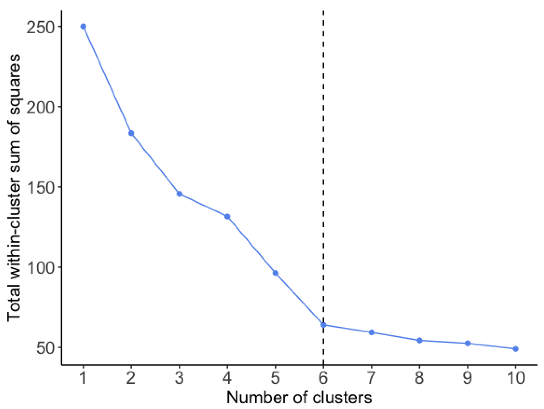
In particular, the standard k-means method was used to perform the cluster analysis. The k-means method [23] is an unsupervised machine learning partitioning method that divides n p-dimensional observations , into k clusters. Broadly speaking, the algorithm initializes with k random means and iterates until convergence is reached, i.e., until the elements in each cluster no longer change. An advantage of this method with respect to hierarchical clustering methods is that the elements assigned to one cluster are allowed to change to another, as the iterative process progresses towards convergence. On the other hand, one of its main drawbacks is that a specific number for k has to be specified beforehand. There is no agreement on which criteria is best to determine the optimal number of clusters. A simple approach is the elbow method, which consists in computing the total within-cluster sum of squares for different values of k and subsequently, plotting the results as a function of k. This approach is called the elbow method because the optimal number of clusters is considered to be the k in which the curve bends.
Once the clusters were obtained, the weighted average of each variable (, H) was computed for each cluster, with the proportional area of the PAs belonging to the c-th cluster being used as the weights. Let (with ) be the set of variables , . The weighted average () is computed as
where is the proportion of the i-th PA over the total area of the s elements belonging to the c-th cluster. Note that the weights are normalized since .
3. Results
3.1. Ecosystem Service () and Diversity (H) Variables
The results of the ecosystem service assessment are shown in Table 3. According to the consulted experts, the agricultural ecosystem service is provided by herbaceous crops, woody crops, greenhouses, and heterogeneous lands. Livestock grazing would be generated by woody crops, heterogeneous lands, and grassland. The microclimate regulation service is generated by woody crops, heterogeneous lands, bush, forest, bush-and-forest, and water. The environmental education service is provided by heterogeneous lands, grassland, bush, forest, bush-and-forest, and water. Finally, the tourism service is generated by heterogeneous lands, forest, bush-and-forest, and water.
Therefore, the provisioning, regulating and cultural ESs (i.e., variables ) are generated by the combination of land-uses that generate the individual ESs belonging to each category, i.e., the provisioning ESs considered are generated by herbaceous crops, woody crops, greenhouses, heterogeneous lands, and grassland; while the cultural ESs are generated by heterogeneous lands, grassland, bush, forest, bush and forest and water.
The results of this assessment were used to compute the proportion of cell that generates each individual ES given the distribution of land-uses in each cell of the grid. Figure 3 shows six maps in which the spatial distribution of the ecosystem service variables () and Shannon’s index (H) is represented at the grid scale. These maps can be analyzed according to the geomorphological units shown in Figure 1.
The Baetic Depression shows high values for the Agriculture ES, while Livestock grazing and microclimatic regulation ESs take high values just in the eastern region. Eastern Baetic Depression is largely covered by olive groves, which explains the generation of provisioning ESs and the microclimatic regulation (due to carbon sequestration). Cultural ESs show low values in the entire area. On the other hand, the diversity index also shows lower values in this region.
The Sierra Morena mountain range shows high values of regulating and cultural ESs, with the provisioning ES taking lower values, except for the northernmost region. The border between Sierra Morena and the Baetic depression is clearly visible. Regarding the diversity index, cells lying in this region seem to take slightly higher values than those falling in the Baetic Depression.
The Baetic systems present higher variability than the aforementioned geomorphological units. Regarding variables and , the higher values correspond to cells located at a lower elevation, which are closer to the Baetic Depression, with woody crops (particularly olive groves) and rain-fed herbaceous crops being the main land-uses. With respect to the variable, most of the Baetic Systems take high values, with the exception of the low-lying areas, especially the easternmost part, where herbaceous crops dominate. Regarding the cultural ecosystem services and the diversity index, higher values generally correspond to cells lying in protected areas (Figure 1).
Finally, the Littoral presents low values of , with the exception of a region dominated by greenhouses (the so-called “sea of plastic” of Almeria, located in the Southeast). and , except for the westernmost part, which corresponds with the Doñana National and Natural Parks, also present low values. On the other hand, the westernmost part of the Littoral (i.e., the Atlantic Littoral) excels at having higher terrestrial vertebrate diversity index.
3.2. Description of the Protected Areas
The proportion of protected area (PA) that generates each individual ecosystem service () given the distribution of land-uses was obtained. On the other hand, the average value of the Shannon’s diversity index (H) within each PA was computed. Table 4 shows the value of these variables per PA. The results show that Sierras Subbéticas Natural Park (number 11) presents the highest value of and , with 44.3% and 52.1%, respectively, while Bahía de Cádiz Natural Park (number 23) shows the lowest value of these 2 variables, with 0.3% and 1%, respectively. Regarding the variable, Sierra de Hornachuelos Natural Park (number 3) presents the highest value (97.5%), while Del Estrecho Natural Park (number 25) shows the lowest value (67.9%). Concerning the variable, Sierra de Andújar Natural Park (number 5) presents the highest value (97.8%), while Sierras Subbéticas Natural Park (number 11) shows the lowest (61.2%). With respect to the variable, Bahía de Cádiz Natural Park (number 23) presents the highest value (92.4%), while Cabo de Gata - Níjar Natural Park (number 26) shows the lowest (7%). Finally, Bahía de Cádiz Natural Park (number 23) presents the highest value of H (1.541), while Sierra María - Los Vélez shows the lowest value (1.022).
Figure 4 shows the boxplots of the values presented in Table 4. Variable has a minimum value of 0.003, maximum of 0.443, median of 0.136, mean of 0.167 and standard deviation of 0.135. Variable has a minimum value of 0.010, maximum of 0.521, median of 0.187, mean of 0.2117 and standard deviation of 0.134. Variable has a minimum value of 0.679, maximum of 0.975, median of 0.910, mean of 0.884 and standard deviation of 0.075. Variable has a minimum value of 0.612, maximum of 0.978, median of 0.926, mean of 0.903 and standard deviation of 0.073. Variable has a minimum value of 0.070, maximum of 0.924, median of 0.732, mean of 0.689 and standard deviation of 0.196. Finally, variable H has a minimum value of 1.022, maximum of 1.541, median of 1.351, mean of 1.344 and standard deviation of 0.106. Regarding the ecosystem service variables, it is noticeable that the provisioning ESs have the lowest values, while , have the lowest variation.
In order to provide an aggregate value for the different ES categories, the individual ESs belonging to the same category were combined. Figure 5 displays the union of the provisioning, regulating, cultural ESs, as well as the average of the H variable per PA. The provisioning ES ranges from 0.010 to 0.526, with the Sierras Subbéticas Natural Park (number 11) presenting the highest number. It is noticeable that three PAs located in the Sierra Morena mountain range present values above 40%, in particular, those corresponding to numbers 1, 2 and 4. The regulating ES coincides with the since we did not consider more regulating ecosystem services. The lowest values correspond to PAs located in the Littoral. The cultural ES ranges from 0.612 to 0.978, with the Sierras Subbéticas Natural Park (number 11) presenting the lowest number and the Sierra de Andújar Natural Park (number 5) the highest value. In general, all PAs present fairly high values, except for the provisioning case, where values are lower and the standard deviation is higher, i.e., the variability is higher.
3.3. Cluster Analysis
The 26 protected areas were grouped according to their landscape. In order to do that, the percentage of each landscape unit (LSU) within each PA was computed and only the most frequent LSU in each PA was used for the cluster analysis.
The Elbow method was used to determine the optimal number of clusters before carrying out the cluster analysis. Figure 6 shows the plot of the within-cluster sum of square, i.e., the variance within the groups, for each value of k from 1 to 10. According to the method used, the optimal number of clusters is 6.
As the data were standardized before running the cluster analysis (i.e., transformed to variables with mean 0 and variation 1, whose values are called z-scores), the cluster means are also standardized and represent standard deviations from the mean. For instance, a z-score of 0 indicates that the value of the original variable coincides with the mean, whereas negative z-scores correspond with values of the variable lower than the mean and positive z-scores with values higher than the mean.
The cluster analysis revealed some characteristics of the six groups. Table 5 shows the cluster means of each variable (LSU) used to run the cluster analysis and Figure 7 depicts the membership of the PAs to the different clusters. The first cluster is composed of five PAs and is characterized by landscapes dominated by scrubland-with-forest (cluster mean = 0.86) and scrubland (cluster mean = 1.31). The second cluster only has 1 PA, corresponding with Cabo de Gata Natural Park, which is characterized by volcanic landscapes (cluster mean = 4.9). The third cluster is composed of four PAs (all of them located in the West coast of the study area) and is characterized by natural marshes (cluster mean = 2.13), salty marshes (cluster mean = 1.28) and dunes and sandbanks (cluster mean = 1.94). The fourth cluster comprises three PAs (all of them located in the Sierra Morena Mountain range) and is characterized by the dominance of dehesa (cluster mean = 2.58) and scrubland (cluster mean = 0.66). The fifth cluster is the largest, comprising seven PAs, and is characterized by limestone formations (cluster mean = 1.29) and scrubland with forest (cluster mean = 0.52). The sixth cluster contains six PAs, characterized by pines and conifers (cluster mean = 1.37) and naked soil and snowfield (cluster mean = 0.68). To summarize, we can say that cluster 1 corresponds to regions dominated by scrubland; cluster 2 to volcanic lands; cluster 3 to marshes; cluster 4 to dehesas; cluster 5 to limestone areas; and cluster 6 to regions dominated by pines and conifers.
Regarding the remainder LSU (which were not used to run the cluster analysis because they are not dominant in the PA) it is noticeable that olive groves present an over-average mean z-score in clusters 4 and 5 (0.402 and 0.589, respectively), with the other clusters being below the mean (negative z-score).
Table 6 shows the weighted average of each variable (, H) within each cluster, as well as the proportional area of each PA over the total area of PAs belonging to a given cluster. It can be noted that, on average, the area that generates the , and ecosystem services is greater in PAs belonging to cluster 4, where the dehesa landscape dominates. In the case of the provisioning ESs, cluster 4 takes relatively high values (0.412 and 0.436) in comparison to the second best cluster (cluster 5), which takes 0.199 for and 0.257 for . On the other hand, the and ESs are more extended in PAs belonging to cluster 1, where scrubland landscapes dominate. Finally, the diversity of taxonomic vertebrate classes shows very similar values in all clusters, with cluster 2 presenting the highest value.
4. Discussion
Dehesa systems and extensive olive groves are the main typologies of cultural landscapes in Natural Parks of Andalusia (Figure 5 and Figure 7). Dehesa systems in Natural Parks of Aracena y Picos de Aroche (number 1), Sierra Norte (number 2), and Cardeña Montoro (number 4) are representative of wood pastures with herbaceous crops, while Hornachuelos Natural Park (number 3) shows wood-pastures with herbaceous crops and more presence of scrubland. In these landscapes, grazing livestock (sheep, cattle and Iberian pig) is the main contribution to food production. In Sierra Norte, there are 1200 livestock farms of Iberian pig and, where 70,000 Iberian pigs were slaughtered in the period 2017–2018. Sierra de Andújar (number 5) and Alcornocales (number 16) Natural Parks represent wood pastures with a high density of scrubland, making grazing more difficult. Although these systems are excellent examples to explore and study how farmlands could be incorporated into conservation, the strategies of conservation by regional administrations are focused on particular interventions, avoiding holistic and integrative approaches. In this sense, FAO [24] considers the need for a holistic approach to food production that opens the way for the successful integration of protected areas, agriculture, and livestock. This consideration emphasizes the importance of cultural landscapes, inside PAs, as food providers, having an important role in food security.
Dehesa systems need specific and constant management, related to grazing livestock, forest and land-use changes [17]:
- For grazing livestock it is necessary to limit the grazing pressure, i.e., the grazing regime should allow time and space gaps between grazing activities and relevant practices, in order to ensure tree regeneration [17].
- Particular forest management practices are needed. Trees are valued not only for wood production but also for the shade and food they provide [25], such as fruits or acorns for Iberian pigs. Note that the effects of trees on pasture production are strongly context-dependent and range from neutral to negative for evergreen oak [26,27].
- Abandonment and intensification are two opposed tendencies in land-use changes. The abandonment of dehesas is the result of rural marginalization and decline of livestock farming [28]. Therefore, there is a high rate of emigration, mainly of young people, seeking better job opportunities in larger cities [29]. Consequently, the population progressively ages and the birth rate falls. These social characteristics are representative of the evolution of Sierra Norte Natural Park. Currently, the population is stable mainly due to rural tourism and the industry derived from Iberian pig grazing. The abandonment of dehesas entails the development of ecological succession, which implies an increase of scrubland and a loss of heterogeneity. The intensification through overgrazing is probably the most important driver of wood pasture loss [24]. A decline in pastures implies an increase in soil erosion [30]. In the studied Natural Parks, overgrazing is controlled by park managers, by avoiding the increase of livestock grazing that affects wood pastures.
In Andalusia, olive groves (plantations of Olea europaea L.) cover 1.5 × 10⁶ ha (14% of olive groves are located in protected areas, mainly Natural Parks). The Natural Park with the largest area covered by olive groves is Sierras Subbéticas (35.13%), followed by Sierra Mágina (15.16%). The remaining Natural Parks present a cover of olive groves lower than 8%. It should be noted that Natural Parks with dominance of dehesa landscape have some amount of protected ground dedicated to olive groves (Sierra Norte de Sevilla: 8.76%; Sierra Aracena y Picos de Aroche: 4.55%; Hornachuelos: 1.61%) [31].
The Natural Park Sierras Subbéticas is representative of cultural landscapes of olive groves. The population of the municipalities of the area of influence of this Natural park in 2002 is 70,067 inhabitants, which makes this PA the most populated Natural Park in Andalusia. Population in this area is aging and, on average, has lower education level due to difficulties in accessing educational resources [14]. As in other regions, inside or outside Natural Parks of Andalusia, the profitability of olive crops has shown a marked decrease, leading farmers either to intensify management practices or to abandon their farms [32]. Abandonment causes a disruption in regulating services by increasing biomass (scrub encroachment), and, therefore, enhances the risk of fire [33]. Intensification (increase in planting density, use of agro-chemicals), affects regulating ecosystem services, due to erosion and atmospheric pollution among others [34], and has a negative impact on biodiversity [35].
The spatial planning of agricultural landscapes looks for an appropriate relationship between spatial heterogeneity, agricultural production and biodiversity conservation. Two approaches to guarantee food production and biodiversity conservation have been proposed in recent years: land sharing and land sparing [36,37]. Briefly, the land sharing approach implies to integrate agricultural production and biodiversity conservation on the same land, while the land sparing scheme separates high-yield farming, maintaining PAs from conversion to agriculture [38]. Ref. [39] studies two different areas in Andalusia: Estepa (a non-protected area) and Sierra de Segura (which is part of the Sierras de Cazorla, Segura y Las Villas Natural Park). For the non-protected area, this work proposes the land sharing strategy because olive groves cover an almost continuous patch of over 60% of their study area. For the protected area, which has a wide area covered by native vegetation (more than 75%), the authors propose that farmers assume the land-sparing option, so that the administration uses environmental subsidies to support farmers [40].
The results also show the role of protected cultural landscapes as providers of cultural ecosystem services (Figure 5). Currently, there is a strong demand for cultural ecosystem services within PAs among urban and rural communities, mainly tourism, which is expected to grow further [41]. As future work, the magnitude of supply and demand of ESs could be studied to explore possible trade-offs or synergies among different end-users (such as tourist and locals) and examine their influence in the delivery of ecosystem services. On the other hand, the results highlight the importance of cultural landscapes in microclimate regulation [42]. In addition, Figure 5 shows that cultural landscapes, as part of PAs, are essential for biodiversity conservation [43,44,45].
The results obtained in this study emphasize the importance of cultural landscapes, inside PAs, as food providers. These results can be generalized to the Mediterranean region. In the European Union, the Habitats Directive is the instrument for wildlife and nature conservation [46]. Ref. [17] consider that only four habitat types (including dehesas) are explicitly recognized as grazed woody formations in the Directive (Annex I). The analysis of these authors highlights that 27.6% of the wood-pastures of the European Union are included in the Natura 2000 network, mainly in the Mediterranean region. Although the aim of the Directive is to maintain and restore favorable conservation status of natural habitats of wild fauna and flora of community interest, there is a need to introduce all typology of cultural landscapes in the Natura 2000 network. In this way, not only biological conservation or regulation or cultural ecosystem services will be considered inside PAs but also food supply and security.
5. Conclusions
Cultural landscapes, inside PAs, play an important role not only for biodiversity conservation but also as providers of cultural and regulating ecosystem services. In general, the importance of provisioning ecosystem services in PAs is less recognized. Dehesa systems and olive groves are key cultural landscapes for food production and should play an important role in the development of the Sustainable Development Goals of the United Nations. Although there are international agreements on the preservation of these landscapes (for instance, The European Landscape Convention) [47], the management of biodiversity conservation and agriculture at the regional scale depends on different administrations, making the planning of these landscapes difficult. Therefore, the integration of conservation strategies with sustainable agriculture is necessary, with a holistic and integrative view of these systems.
In Andalusia, abandonment of these landscapes is one of the most important drivers of change. In order to avoid this tendency, the new Common Agriculture Policy post-2020 should pay specific attention to farmers inside PAs, who are engaged in environmental-friendly agriculture and work in partnership with PA managers and politicians, by recognizing their work and rewarding their efforts, establishing specific funds for the maintenance of these landscapes.
Author Contributions
Conceptualization, P.A.A.; Methodology, A.D.M. and D.R.-L.; Software, A.D.M. and D.R.-L.; Validation, A.D.M., D.R.-L. and P.A.A.; Formal Analysis, A.D.M. and D.R.-L.; Investigation, A.D.M., D.R.-L. and P.A.A.; Writing—Original Draft Preparation, A.D.M. and P.A.A.; Writing— review & editing, D.R.-L.; Supervision, A.D.M., D.R.-L. and P.A.A.
Funding
This research received no external funding.
Acknowledgments
DRL thanks the support from CDTIME (University of Almería), the research group FQM-229, and from Campus de Excelencia Internacional del Mar (CEIMAR) of the University of Almería.
Conflicts of Interest
The authors declare no conflict of interest.
References
- Convention on Biological Diversity; United Nations: New York, NY, USA, 1992.
- Palomo, I.; Montes, C.; Martín-López, B.; González, J.A.; García-Llorente, M.; Alcorlo, P.; García Mora, M.R. Incorporating the social-ecological approach in protected areas in the Anthropocene. BioScience 2014, 64, 181–191. [Google Scholar] [CrossRef]
- Dudley, N. (Ed.) Guidelines for Applying Protected Area Management Categories; IUCN: Gland, Switzerland, 2008; 86p. [Google Scholar]
- Kareiva, P.; Marvier, M. Conservation Science. Balancing the Needs of People and Nature; Roberts and Company Publishers: Englewood, CO, USA, 2015. [Google Scholar]
- Kareiva, P.; Marvier, M. What is conservation science? BioScience 2012, 62, 962–969. [Google Scholar] [CrossRef]
- Anderies, J.M.; Janssen, M.A.; Ostrom, E. A framework to analyze the robustness of socio-ecological systems from an institutional perspective. Ecol. Soc. 2004, 9, 18. [Google Scholar] [CrossRef]
- Ban, N.C.; Mills, M.; Tam, J.; Hicks, C.C.; Klain, S.; Stoeckl, N.; Bottrill, M.C.; Levine, J.; Pressey, R.L.; Satterfield, T.; et al. A social–ecological approach to conservation planning: Embedding social considerations. Front. Ecol. Environ. 2013, 11, 194–202. [Google Scholar] [CrossRef]
- Farina, A. The Cultural Landscape as a Model for the Integration of Ecology and Economics. BioScience 2000, 50, 313. [Google Scholar] [CrossRef] [Green Version]
- Rescia, A.; Pérez-Corona, M.E.; Arribas-Ureña, P.; Dover, J. Cultural landscapes as complex adaptive systems: The cases of northern Spain and Northern Argentina. In Resilience and the Cultural Landscape: Understanding and Managing Change in Human-Shaped Environments; Pleninger, T., Bieling, T., Eds.; Cambridge University Press: Cambridge, UK, 2012; pp. 126–145. [Google Scholar]
- Rescia, A.; Willaarts, B.; Schmitz, M.; Aguilera, P. Changes in land uses and management in two Nature Reserves in Spain: Evaluating the social-ecological resilience of natural landscapes. Landsc. Urban Plan. 2010, 98, 26–35. [Google Scholar] [CrossRef]
- Maldonado, A.D.; Ramos-López, D.; Aguilera, P.A. A Comparison of Machine-Learning Methods to Select Socioeconomic Indicators in Cultural Landscapes. Sustainability 2018, 10, 4312. [Google Scholar] [CrossRef]
- Schmitz, M.F.; De Aranzabal, I.; Aguilera, P.A.; Rescia, A.; Pineda, F.D. Relationship between landscape typology and socioeconomic structure: Scenarios of change in Spanish cultural landscapes. Ecol. Model. 2003, 168, 343–356. [Google Scholar] [CrossRef]
- De Aranzabal, I.; Schmitz, M.F.; Aguilera, P.; Pineda, F.D. Modelling of landscape changes derived from the dynamics of socio-ecological systems: A case of study in a semiarid Mediterranean landscape. Ecol. Indic. 2008, 8, 672–685. [Google Scholar] [CrossRef]
- Maldonado, A.D.; Aguilera, P.A.; Salmerón, A.; Nicholson, A.E. Probabilistic modeling of the relationship between socioeconomy and ecosystem services in cultural landscapes. Ecosyst. Serv. 2018, 33, 146–164. [Google Scholar] [CrossRef]
- Ferraz-De-Oliveira, M.I.; Azeda, C.; Pinto-Correia, T. Management of Montados and Dehesas for High Nature Value: An interdisciplinary pathway. Agrofor. Syst. 2016, 90, 1–6. [Google Scholar] [CrossRef]
- Bergmeier, E.; Petermann, J.; Schröder, E. Geobotanical survey of woodpasture habitats in Europe: Diversity, threats and conservation. Biodivers. Conserv. 2010, 19, 2995–3014. [Google Scholar] [CrossRef]
- Plieninger, T.; Hartel, T.; Martín-López, B.; Beaufoy, G.; Bergmeier, E.; Kirby, K.; Montero, M.J.; Moreno, G.; Oteros-Rozas, E.; Uytvanck, J.V. Wood-pastures of Europe: Geographic coverage, social–ecological values, conservation management, and policy implications. Biol. Conserv. 2015, 190, 70–79. [Google Scholar] [CrossRef]
- Rey Benayas, J.M.; Martins, A.; Nicolau, J.M.; Schulz, J.J. Abandonment of agricultural land: An overview of drivers and consequences. CAB Rev. Perspect. Agric. Vet. Sci. Nutr. Nat. Resour. 2007, 2. [Google Scholar] [CrossRef]
- Plieninger, T.; Hui, C.; Gaertner, M.; Huntsinger, L. The Impact of Land Abandonment on Species Richness and Abundance in the Mediterranean Basin: A Meta-Analysis. PLoS ONE 2014, 9, e98355. [Google Scholar] [CrossRef]
- Stanners, D.; Bourdeau, P.; European Environment Agency; Comisión Europea, Oficina de Publicaciones Oficiales de las Comunidades Europeas. Europe’s Environment: The Dobris Assessment; European Environment Agency: Copenhagen, Denmark, 1995. [Google Scholar]
- Millennium Ecosystem Assessment. Ecosystems and Human Well-Being: Synthesis; Synthesis Reports; Island Press: Washington, DC, USA, 2005. [Google Scholar]
- Legendre, P.; Legendre, L. Numerical Ecology; Elsevier: Amsterdam, The Netherlands, 2012. [Google Scholar]
- Likas, A.; Vlassis, N.; Verbeek, J.J. The global k-means clustering algorithm. Pattern Recognit. 2003, 36, 451–461. [Google Scholar] [CrossRef] [Green Version]
- FAO. Protected Areas, People and Food Security. FAO Contribution to the World Parks Congress, Sidney, Australia; Technical Report; Food and Agriculture Organization of the United Nations: Rome, Italy, 2014; 23p. [Google Scholar]
- Jørgensen, D. Pigs and Pollards: Medieval Insights for UK Wood Pasture Restoration. Sustainability 2013, 5, 387–399. [Google Scholar] [CrossRef] [Green Version]
- Rivest, D.; Paquette, A.; Moreno, G.; Messier, C. A meta-analysis reveals mostly neutral influence of scattered trees on pasture yield along with some contrasted effects depending on functional groups and rainfall conditions. Agric. Ecosyst. Environ. 2013, 165, 74–79. [Google Scholar] [CrossRef]
- Gea-Izquierdo, G.; Montero, G.; Cañellas, I. Changes in limiting resources determine spatio-temporal variability in tree–grass interactions. Agrofor. Syst. 2009, 76, 375–387. [Google Scholar] [CrossRef]
- Plieninger, T.; Bieling, C. Resilience-Based Perspectives to Guiding High-Nature-Value Farmland through Socioeconomic Change. Ecol. Soc. 2013, 18. [Google Scholar] [CrossRef] [Green Version]
- Fischer, J.; Hartel, T.; Kuemmerle, T. Conservation policy in traditional farming landscapes. Conserv. Lett. 2012, 5, 167–175. [Google Scholar] [CrossRef] [Green Version]
- Moreno, G.; Pulido, F.J. The Functioning, Management and Persistence of Dehesas. In Agroforestry in Europe. Current Status and Future Prospects; Rigueiro-Rodrguez, A., Mosquera, M., McAdam, J., Eds.; Springer: Heidelberg/Berlin, Germany; New York, NY, USA, 2009; pp. 127–160. [Google Scholar]
- Gúzman Álvarez, J.R. Territorio y Medio Ambiente en el Olivar Andaluz; Olivicultura y Elaiotécnica, Junta de Andalucía: Sevilla, Spain, 2005. [Google Scholar]
- Sánchez Martínez, J.; Gallego Simón, V.; Araque Jiménez, E. El olivar andaluz y sus trasformaciones recientes. Estud. Geogr. 2011, 270, 203–229. [Google Scholar] [CrossRef]
- Sousa, A.A.R.; Barandica, J.M.; Sanz-Cañada, J.; Rescia, A.J. Application of a dynamic model using agronomic and economic data to evaluate the sustainability of the olive grove landscape of Estepa (Andalusia, Spain). Landsc. Ecol. 2019. [Google Scholar] [CrossRef]
- López-Pintor, A.; Sanz-Cañada, J.; Salas, E.; Rescia, A. Assessment of Agri-Environmental Externalities in Spanish Socio-Ecological Landscapes of Olive Groves. Sustainability 2018, 10, 2640. [Google Scholar] [CrossRef]
- Flohre, A.; Fischer, C.; Aavik, T.; Bengtsson, J.; Berendse, F.; Bommarco, R.; Ceryngier, P.; Clement, L.W.; Dennis, C.; Eggers, S.; et al. Agricultural intensification and biodiversity partitioning in European landscapes comparing plants, carabids, and birds. Ecol. Appl. 2011, 21, 1772–1781. [Google Scholar] [CrossRef] [Green Version]
- Phalan, B.; Balmford, A.; Green, R.E.; Scharlemann, J.P. Minimising the harm to biodiversity of producing more food globally. Food Policy 2011, 36. [Google Scholar] [CrossRef]
- Tscharntke, T.; Clough, Y.; Wanger, T.C.; Jackson, L.; Motzke, I.; Perfecto, I.; Vandermeer, J.; Whitbread, A. Global food security, biodiversity conservation and the future of agricultural intensification. Biol. Conserv. 2012, 151, 53–59. [Google Scholar] [CrossRef]
- Ortega, M.; Pascual, S.; Rescia, A. Spatial structure of olive groves and scrublands affects Bactrocera oleae abundance: A multi-scale analysis. Basic Appl. Ecol. 2016, 17, 696–705. [Google Scholar] [CrossRef]
- Rescia, A.J.; Ortega, M. Quantitative evaluation of the spatial resilience to the B. oleae pest in olive grove socio-ecological landscapes at different scales. Ecol. Indic. 2018, 84, 820–827. [Google Scholar] [CrossRef]
- Rescia, A.J.; Sanz-Cañada, J.; Bosque-González, I.D. A new mechanism based on landscape diversity for funding farmer subsidies. Agron. Sustain. Dev. 2017, 37. [Google Scholar] [CrossRef]
- Milcu, A.I.; Hanspach, J.; Abson, D.; Fischer, J. Cultural Ecosystem Services: A Literature Review and Prospects for Future Research. Ecol. Soc. 2013, 18. [Google Scholar] [CrossRef] [Green Version]
- Power, A.G. Ecosystem services and agriculture: Tradeoffs and synergies. Philos. Trans. R. Soc. B Biol. Sci. 2010, 365, 2959–2971. [Google Scholar] [CrossRef]
- Baiamonte, G.; Domina, G.; Raimondo, F.M.; Bazan, G. Agricultural landscapes and biodiversity conservation: A case study in Sicily (Italy). Biodivers. Conserv. 2015, 24, 3201–3216. [Google Scholar] [CrossRef]
- Hanspach, J.; Loos, J.; Dorresteijn, I.; Abson, D.J.; Fischer, J. Characterizing social-ecological units to inform biodiversity conservation in cultural landscapes. Divers. Distrib. 2016, 22, 853–864. [Google Scholar] [CrossRef]
- Moreno, G.; Gonzalez-Bornay, G.; Pulido, F.; Lopez-Diaz, M.L.; Bertomeu, M.; Juárez, E.; Diaz, M. Exploring the causes of high biodiversity of Iberian dehesas: The importance of wood pastures and marginal habitats. Agrofor. Syst. 2015, 90, 87–105. [Google Scholar] [CrossRef]
- Directive, H. Council Directive 92/43/EEC of 21 May 1992 on the conservation of natural habitats and of wild fauna and flora. Off. J. Eur. Union 1992, 206, 7–50. [Google Scholar]
- Council of Europe. European Landscape Convention. Report and Convention; Council of Europe: Strasbourg, France, 2000. [Google Scholar]
Figure 1.
Natural and national parks of the study area. The main geomorphological units are shown. 1: Sierra de Aracena y Picos de Aroche; 2: Sierra Norte de Sevilla; 3: Sierra de Hornachuelos; 4: Sierra de Cardeña y Montoro; 5: Sierra de Andújar; 6: Despeñaperros; 7: Sierras de Cazorla, Segura y Las Villas; 8: Sierra de Castril; 9: Sierra Mágina; 10: Sierra María-Los Vélez; 11: Sierras Subbéticas; 12: Sierra de Huétor; 13: Sierra de Baza; 14: Sierra Nevada (National Park); 15: Sierra Nevada; 16: Los Alcornocales; 17: Sierra de Grazalema; 18: Sierra de las Nieves; 19: Montes de Málaga; 20: Sierras de Tejeda, Almijara y Alhama; 21: Doñana; 22: Doñana (National Park); 23: Bahía de Cádiz; 24: La Breña y Marismas del Barbate; 25: Del Estrecho; 26: Cabo de Gata-Níjar.

Figure 2.
Venn diagrams representing 2 logical relationships (union and intersection) between 2 ecosystem services. Each circle represents an ES, i.e., the region of the space where they occur. The union represents the combined region of both ES, while the intersection represents the region where both ES occur simultaneously.

Figure 3.
Ecosystem service variables () and Shannon’s index (H). Main geomorphological units are outlined in black color. Note that variables range from 0 to 1, while H ranges from 0 to 2. Agr, agriculture; LG, livestock grazing; MCR, microclimatic regulation; EnvEd, environmental education; Tour, tourism; H, Shannon’s index.

Figure 4.
Boxplot of the ecosystem service () and diversity (H) variables obtained from Table 4. Outliers are labeled with the corresponding PA number.
Figure 4.
Boxplot of the ecosystem service () and diversity (H) variables obtained from Table 4. Outliers are labeled with the corresponding PA number.

Figure 5.
Union of the provisioning ( and ), regulating () and cultural ( and ) ecosystem services generated in each protected area. Shannon’s index H is also represented. The numerical values of the individual variables can be referred to in Table 4. Note that the scale is different in each map.
Figure 5.
Union of the provisioning ( and ), regulating () and cultural ( and ) ecosystem services generated in each protected area. Shannon’s index H is also represented. The numerical values of the individual variables can be referred to in Table 4. Note that the scale is different in each map.

Figure 6.
Elbow method to determine the optimal number of clusters. k = 6 is the optimal.

Figure 7.
Clusters of protected areas found after applying the k-means algorithm. Cluster 1: scrubland; cluster 2: volcanic lands; cluster 3: marshes; cluster 4: dehesas; cluster 5: limestone; and cluster 6: pines and conifers.
Figure 7.
Clusters of protected areas found after applying the k-means algorithm. Cluster 1: scrubland; cluster 2: volcanic lands; cluster 3: marshes; cluster 4: dehesas; cluster 5: limestone; and cluster 6: pines and conifers.


Table 1.
Land-use SIOSE categories, obtained from the Land use and vegetation cover map of Andalusia, and their corresponding aggregated categories, .
Table 1.
Land-use SIOSE categories, obtained from the Land use and vegetation cover map of Andalusia, and their corresponding aggregated categories, .
| SIOSE Category | Aggregated Land-Use Variables, |
|---|---|
| Urban mix | Built |
| Industrial | |
| Mining | |
| Transport | |
| Technical infrastructures | |
| Herbaceous crops | Herbaceous crops |
| Greenhouses | Greenhouses |
| Woody crops | Woody crops |
| Mixtures of crops and natural vegetations | Heterogeneous lands |
| Grassland with forest | |
| Grassland | Grassland |
| Bush | Bush |
| Forest | Forest |
| Bush and forest | Bush and forest |
| Naked soil | Naked soil |
| Bodies of water | Bodies of water |
Table 2.
Landscape units (LSUs) provided by the Landscape Map of Andalusia.
| Type of Landscape | |||
|---|---|---|---|
| Natural | Agricultural | Artificial | Geomorphological |
| Pines and conifers | Olive groves | Urban | Naked soil and snowfields |
| Oaks | Almond groves | Mine and dump | Volcanic lands |
| Scrubland with forest | Vineyards | Salt marshes and aquaculture crops | Cliffs |
| Riparian vegetation | Arable lands | Reservoirs and waterbodies | Meadows |
| Eucalyptus groves | Irrigated fruit trees | Gullies | |
| Scrubland | Irrigated crops | Malpais | |
| Esparto fields | Ricefields | Limestone formations | |
| Grassland | Greenhouses | Mesa and cuesta | |
| Wasteland | Delta | ||
| Dehesa | Beaches | ||
| Natural marshes | Dunes and sandbanks | ||
Table 3.
Ecosystem service assessment. At least 80% of the experts consulted agree that land-use generates ecosystem service (1) or not (0). Ecosystem services: Agr, agriculture; LG, livestock grazing; MCR, microclimate regulation; EnvEd, environmental education; Tour, tourism. Land-uses: Herb, herbaceous crops, GH, greenhouses, Woody, woody crops; Het, heterogeneous lands.
| Ecosystem Service | Type | Built | Herb | GH | Woody | Het | Grassland | Bush | Forest | Bush & Forest | Naked Soil | Water |
|---|---|---|---|---|---|---|---|---|---|---|---|---|
| Agr | Provisioning | 0 | 1 | 1 | 1 | 1 | 0 | 0 | 0 | 0 | 0 | 0 |
| LG | Provisioning | 0 | 0 | 0 | 1 | 1 | 1 | 0 | 0 | 0 | 0 | 0 |
| MCR | Regulating | 0 | 0 | 0 | 1 | 1 | 0 | 1 | 1 | 1 | 0 | 1 |
| EnvEd | Cultural | 0 | 0 | 0 | 0 | 1 | 1 | 1 | 1 | 1 | 0 | 1 |
| Tour | Cultural | 0 | 0 | 0 | 0 | 1 | 0 | 0 | 1 | 1 | 0 | 1 |
Table 4.
Proportion of protected area (PA) that generates each ecosystem service and mean value of diversity of terrestrial vertebrates in each PA. Boldfaced numbers indicate the highest value per column whereas numbers in italics show the lowest values. PAs are organized according to the Main Geomorphological Units (MGU) to improve readability.
| MGU | Protected Area | Agr | LG | MCR | EnvEd | Tour | H |
|---|---|---|---|---|---|---|---|
| SIERRA MORENA MOUNTAIN RANGE | 1. Sierra de Aracena y Picos de Aroche | 0.384 | 0.409 | 0.916 | 0.884 | 0.744 | 1.382 |
| 2. Sierra Norte de Sevilla | 0.440 | 0.464 | 0.917 | 0.869 | 0.761 | 1.317 | |
| 3. Sierra de Hornachuelos | 0.236 | 0.238 | 0.975 | 0.965 | 0.846 | 1.166 | |
| 4. Sierra de Cardeña y Montoro | 0.421 | 0.433 | 0.944 | 0.947 | 0.897 | 1.344 | |
| 5. Sierra de Andújar | 0.185 | 0.231 | 0.932 | 0.978 | 0.741 | 1.423 | |
| 6. Despeñaperros | 0.088 | 0.096 | 0.947 | 0.941 | 0.866 | 1.461 | |
| BAETIC SYSTEMS | 7. Sierras de Cazorla, Segura y Las Villas | 0.201 | 0.223 | 0.930 | 0.884 | 0.723 | 1.428 |
| 8. Sierra de Castril | 0.093 | 0.268 | 0.797 | 0.953 | 0.525 | 1.451 | |
| 9. Sierra Mágina | 0.263 | 0.292 | 0.948 | 0.840 | 0.643 | 1.276 | |
| 10. Sierra María-Los Vélez | 0.188 | 0.148 | 0.897 | 0.859 | 0.711 | 1.022 | |
| 11. Sierras Subbéticas | 0.443 | 0.521 | 0.884 | 0.612 | 0.351 | 1.208 | |
| 12. Sierra de Huétor | 0.047 | 0.072 | 0.925 | 0.956 | 0.784 | 1.294 | |
| 13. Sierra de Baza | 0.147 | 0.187 | 0.890 | 0.931 | 0.685 | 1.343 | |
| 14. Sierra Nevada (National Park) | 0.027 | 0.152 | 0.786 | 0.910 | 0.394 | 1.269 | |
| 15. Sierra Nevada | 0.199 | 0.223 | 0.904 | 0.889 | 0.632 | 1.281 | |
| 16. Los Alcornocales | 0.125 | 0.153 | 0.898 | 0.946 | 0.814 | 1.435 | |
| 17. Sierra de Grazalema | 0.278 | 0.319 | 0.845 | 0.880 | 0.726 | 1.355 | |
| 18. Sierra de las Nieves | 0.053 | 0.188 | 0.825 | 0.955 | 0.588 | 1.318 | |
| 19. Montes de Málaga | 0.062 | 0.066 | 0.953 | 0.922 | 0.896 | 1.277 | |
| 20. Sierras de Tejeda, Almijara y Alhama | 0.045 | 0.069 | 0.934 | 0.953 | 0.631 | 1.384 | |
| LITTORAL | 21. Doñana | 0.143 | 0.125 | 0.819 | 0.852 | 0.777 | 1.346 |
| 22. Doñana (National Park) | 0.046 | 0.125 | 0.857 | 0.937 | 0.737 | 1.411 | |
| 23. Bahía de Cádiz | 0.003 | 0.010 | 0.935 | 0.942 | 0.924 | 1.541 | |
| 24. La Breña y Marismas del Barbate | 0.011 | 0.033 | 0.939 | 0.962 | 0.923 | 1.383 | |
| 25. Del Estrecho | 0.076 | 0.276 | 0.679 | 0.880 | 0.524 | 1.421 | |
| 26. Cabo de Gata-Níjar | 0.129 | 0.165 | 0.717 | 0.833 | 0.070 | 1.405 |
Table 5.
Cluster mean values of the 10 dominant landscapes used to perform the cluster analysis. The presented values are z-scores. Boldfaced numbers indicate high z-score values per column, revealing the landscapes that characterize each cluster.
Table 5.
Cluster mean values of the 10 dominant landscapes used to perform the cluster analysis. The presented values are z-scores. Boldfaced numbers indicate high z-score values per column, revealing the landscapes that characterize each cluster.
| Cluster | 1 | 2 | 3 | 4 | 5 | 6 | |
|---|---|---|---|---|---|---|---|
| Landscape | |||||||
| Scrubland with forest | 0.864 | −1.570 | −1.572 | −0.021 | 0.522 | −0.009 | |
| Dehesa | 0.034 | −0.475 | −0.475 | 2.580 | −0.387 | −0.472 | |
| Scrubland | 1.311 | −0.265 | −0.718 | 0.658 | −0.187 | −0.681 | |
| Limestone formations | −0.739 | −0.745 | −0.745 | −0.745 | 1.294 | 0.100 | |
| Pines and conifers | −0.315 | −0.822 | −0.494 | −0.397 | −0.384 | 1.375 | |
| Natural marshes | −0.388 | −0.388 | 2.134 | −0.388 | −0.388 | −0.388 | |
| Salty marshes | −0.237 | −0.169 | 1.285 | −0.237 | −0.237 | −0.237 | |
| Volcanic lands | −0.196 | 4.903 | −0.196 | −0.196 | −0.196 | −0.196 | |
| Dunes and sandbanks | −0.286 | −0.181 | 1.945 | −0.386 | −0.386 | −0.386 | |
| Naked soil and snowfield | −0.205 | −0.205 | −0.205 | −0.205 | −0.205 | 0.683 | |
Table 6.
Weighted average of the variables () per cluster of PAs. Bold-faced numbers indicate the highest weighted average value of each variable.
Table 6.
Weighted average of the variables () per cluster of PAs. Bold-faced numbers indicate the highest weighted average value of each variable.
| WEIGHTED AVERAGE | ||||||||
|---|---|---|---|---|---|---|---|---|
| Cluster | Protected Area | Prop. Area | Agr | LG | MCR | EnvEd | Tour | H |
| 1 | 3. Sierra de Hornachuelos | 0.157 | 0.189 | 0.914 | 0.955 | 0.796 | 1.383 | |
| 5. Sierra de Andújar | ||||||||
| 6. Despeñaperros | ||||||||
| 16. Los Alcornocales | ||||||||
| 25. Del Estrecho | ||||||||
| 2 | 26. Cabo de Gata - Níjar | 0.129 | 0.165 | 0.717 | 0.833 | 0.07 | 1.405 | |
| 3 | 21. Doñana | 0.09 | 0.114 | 0.847 | 0.895 | 0.777 | 1.388 | |
| 22. Doñana (National Park) | ||||||||
| 23. Bahía de Cádiz | ||||||||
| 24. La Breña y Marismas del Barbate | ||||||||
| 4 | 1. Sierra de Aracena y Picos de Aroche | 0.412 | 0.436 | 0.919 | 0.883 | 0.766 | 1.350 | |
| 2. Sierra Norte de Sevilla | ||||||||
| 4. Sierra de Cardeña y Montoro | ||||||||
| 5 | 8. Sierra de Castril | 0.199 | 0.257 | 0.882 | 0.876 | 0.620 | 1.335 | |
| 9. Sierra Mágina | ||||||||
| 11. Sierras Subbéticas | ||||||||
| 13. Sierra de Baza | ||||||||
| 17. Sierra de Grazalema | ||||||||
| 18. Sierra de las Nieves | ||||||||
| 20. Sierras de Tejeda, Almijara y Alhama | ||||||||
| 6 | 7. Sierras de Cazorla, Segura y Las Villas | 0.158 | 0.198 | 0.895 | 0.892 | 0.641 | 1.339 | |
| 10. Sierra María - Los Vélez | ||||||||
| 12. Sierra de Huétor | ||||||||
| 14. Sierra Nevada (National Park) | ||||||||
| 15. Sierra Nevada | ||||||||
| 19. Montes de Málaga | ||||||||
© 2019 by the authors. Licensee MDPI, Basel, Switzerland. This article is an open access article distributed under the terms and conditions of the Creative Commons Attribution (CC BY) license (http://creativecommons.org/licenses/by/4.0/).
Share and Cite
MDPI and ACS Style
Maldonado, A.D.; Ramos-López, D.; Aguilera, P.A. The Role of Cultural Landscapes in the Delivery of Provisioning Ecosystem Services in Protected Areas. Sustainability 2019, 11, 2471. https://doi.org/10.3390/su11092471
AMA Style
Maldonado AD, Ramos-López D, Aguilera PA. The Role of Cultural Landscapes in the Delivery of Provisioning Ecosystem Services in Protected Areas. Sustainability. 2019; 11(9):2471. https://doi.org/10.3390/su11092471
Chicago/Turabian StyleMaldonado, Ana D., Darío Ramos-López, and Pedro A. Aguilera. 2019. "The Role of Cultural Landscapes in the Delivery of Provisioning Ecosystem Services in Protected Areas" Sustainability 11, no. 9: 2471. https://doi.org/10.3390/su11092471
Note that from the first issue of 2016, this journal uses article numbers instead of page numbers. See further details here.