Article

Identification of Marginal Landscapes as Support for Sustainable Development: GIS-Based Analysis and Landscape Metrics Assessment in Southern Italy Areas

by
Elena Cervelli
*,
Ester Scotto di Perta
and
Stefania Pindozzi
*
Department of Agricultural Sciences, University of Naples Federico II, Portici 80055, Italy
*
Authors to whom correspondence should be addressed.
Sustainability 2020, 12(13), 5400; https://doi.org/10.3390/su12135400
Submission received: 3 June 2020 / Revised: 26 June 2020 / Accepted: 29 June 2020 / Published: 3 July 2020
(This article belongs to the Special Issue Landscape Analysis, Planning and Regional Development)

Abstract

:
Landscape is increasingly characterized by a multifaced nature. In scientific literature and landscape governance, new landscape definitions are often coined to explain new meanings and to define specific intervention strategies and tools. The present study purposes a framework for the identification of hybrid landscapes as support for land-use planners, which aim to guarantee development opportunities as well as natural heritage preservation and valorization. “Marginal lands” were identified starting from EU Directives and scientific approaches, by means of multicriteria analysis. Different scenarios were built: (1) no-change; (2) energy crops; (3) green infrastructures. An ecosystem services approach, via landscape metrics analysis, was used to compare the possible effects of scenarios. About 20% of the study area, an internal area of the southern Apennines, was identified as suitable for land-use change in a medium-short time, and scenarios of land-use changes show a better condition, in terms of fragmentation, than as a current asset. Results showed the strategic role and potentialities of marginal lands, as a trade-off between nature conservation and development issues, suggesting new opportunities for green infrastructures and a renewable energies chain. The study allowed for deepening the close connection among landscape planning approaches, land use change scenarios building and environmental assessment, focused on the ex-ante evaluation stage.

1. Introduction

Most of the European landscape cannot be understood as simply places [1,2,3] with specific and defined spatial, functional and perceptive features; there are areas with closed interaction between urban and rural functions, or with problems of fragmentation, abandonment, pollution or a low level of productivity. Landscape planning policy-making processes, normally, have produced policies ignoring the real nature of hybrid territories, often with dramatic consequences for the environment. Thus, in the last decades, in addition to the traditional physical classifications of the landscape, based on the “urban” and “rural” dichotomy, further definitions were proposed referring to the concept of “middle landscape”: tussenland [4], città diffusa [5], spread city [6], shadowlands [7], etc. The different names given to the new forms of spatial configurations imply new meanings but also involve the need for specific management and planning approaches, mostly linked to their intrinsic characteristics and value.
Initially these new landscape types were seen only as problems, as conditions of disadvantage to be remedied; however, the most recent theories, are also considering them as opportunities, as new frontiers to guarantee development and sustainability.
Among the middle landscapes, lands with inherent disadvantages or lands marginalized by natural and/or artificial forces, but which have great potential for transformation, the so-called “marginal lands” have been extensively investigated and discussed by scientists. They were described generally as areas that are underused [8], difficult to cultivate [9], with low economic value [10], Limbo lands or lands with uncertain status [8,11], degraded lands [12] and lands with varied developmental potential [13,14].
Less favored areas (LFA), as defined since the 1970s (and still in use today) by the European Economic Community (EEC) Directive 75/268, article 3, paragraph 3–5 [15], then into Regulation 950/97, Regulation 1257/1999 and the Council Regulation EC 1698/2005 [16,17,18], reflecting the negative meaning associated with these contexts, certainly fall within the marginal lands category. The EU Scheme tried to meet the widely divergent regional situations of EU agriculture, with respect to both the socio-economic situation and natural characteristics [19]. Inside LFA, agricultural productions or activities present more difficulties because of natural handicaps such as difficult climatic conditions, steep slopes in mountain areas or low soil productivity, and because of socio-economic problems such as low population densities and low agricultural incomes [20]. Already in these terms, LFAs can offer important solutions and opportunities in the maintenance and management of the agroforest landscape: rural activities, agricultural ones in particular, have high importance for the production, the care and use of landscape, the maintenance of traditional social structures, as well as a multifunctional basis for other economic sectors. On the one hand, mountain agriculture is less able to face market competition, suffering from additional costs and, consequently, needing to sell at higher prices (making it difficult to compete); on the other hand, as a strength and opportunity, mountain agricultural products are characterized by a marked typicality or high quality and by relevant multifunctional activities; primary activity is in many cases the only way of managing areas that are often difficult to maintain [21]. Starting from the EEC Directive 75/268, more than 30 implementing Directives comprise the current delimitation of the LFAs of each Member State. In addition to these classifications, “Territories in between”, often overlooked in the dominant schemes of landscape classification [2], more recently reflect a new approach in land-use and landscape planning, including the hybrid geographies into planning process as areas with specific features as a basis for development opportunities. They help to describe the complex relations between urban and rural landscapes, with new and specific cultural and topographic settings. Their identification starts from demographic and infrastructure/functional assets, underlying the connectivity of places with different functions and uses intensity. Their identification could become a strategic issue in landscape planning, in terms of social relation, environmental protection, mobility, housing and economic activities and overall sustainability [22,23,24].
The identification of middle landscapes is also considered strategic in terms of food security improvement and bioenergy productions support [25,26,27,28]: in addition to the EEC Directive 75/268, other EU policies focus on these contexts (belonging to agroforestry landscape) to improve different issues, such as Biodiversity [29], Green infrastructures [30,31,32] and Renewable energy [33,34]. In this context, many studies debate the “trilemma” of land-use planning in marginal lands: food security, bioenergy and environmental concerns [28,35,36], and require the need for further and more detailed environmental impact analysis, developed according to the most modern theories and approaches. Marginal lands can give a first quantification of the areas in which concentrated measures and interventions, both public and private, can be used for these forms of development. Many approaches and forms of modeling [28,37,38,39,40,41,42,43] were developed to support the identification of land-use change suitable areas and their intensification in land-use [44]. Intensification of land-use on the one hand, and abandonment on the other, could have important consequences for landscape, in terms, for example involving soil erosion, land degradation, biodiversity and climate change mitigation [45,46,47].
The assessment of ecosystem services, which involves the benefits that the population obtains from ecosystems [48,49], is widely considered as a valid support for landscape planning, both in the analysis phase, and in scenario construction and impact assessment phases [50]. The awareness about the development and implementation of related policies (on water, climate, agriculture, forest and regional planning) are the main aims which support the ecosystem services (ESs) approach application. Specifically, in landscape / land-use planning, robust, reliable and comparable data (arising from the different ESs assessment methods developed) are very important, allowing assessing the state of art, comparing scenarios, evaluating environmental damages, etc. Beyond the questions about the classification [49,51,52,53,54,55] of ecosystem services and their assessment methods [56,57,58], a particular role is assumed by landscape metrics, which are able to express easily comparable aspects related to the composition and configuration of the landscape, about the effect (fragmentation, biodiversity, etc.) of land-use changes or about phenomena of abandonment / intensification in land-use immediately and in numerical terms. A landscape metric assessment was used, allowing a critical evaluation of current conditions and giving significant information for guiding decisions toward a sustainable development, according to EU documents. Action 5 of the EU Biodiversity Strategy to 2020 calls Member States to map and assess the state of ecosystems and their services in their national territory with the assistance of the European Commission. In line with the Millennium Ecosystem assessment [49], the objective of the EU assessment is to provide a critical evaluation of the best available information for guiding decisions on complex public issues.
The present study proposes a framework for identification of specific marginal lands in Southern Italy which is scenario-based and landscape metrics based, in order to support land-use and landscape planning activities to achieve sustainable development opportunities, in contexts with socio-economic difficulties but with still high environmental values. The aims of the work are to deepen knowledge about marginal areas in contexts with economic disadvantages, despite their high environmental, cultural and landscape values, and to assess their current resources to support potential land use change or intensity of use. As part of the scientific and operational debate on landscape management, the present study is proposed as part of an ex-ante planning process, acting both at a regional and local level. In particular, on a regional scale, the identification of marginal lands could be inserted structurally in the current territorial and landscape planning tools (i.e., regional or provincial territorial plans), such as what has already been done for areas of environmental value. In this way, the improvement of specific intervention strategies and policies and a transparent and shared support in the distribution of funding and public interventions is possible. At the local level, the identification of marginal lands and the assessment of the possible impact on the landscape of the driving forces could be part of the strategic environmental assessment, together with the existing plans and programs, in order to improve the analysis phase and the efficiency of the planning tools.
Results show specific marginal lands, which represent a discrete class of whole landscape, and can be considered as “in transformation areas”. Marginal lands identified are not simply rural places; instead, they present a general intensification of anthropic functions and need to be inserted in a coordinated development into a large-scale analysis.
Even if the methodology is focused on a specific Mediterranean context, it can also be iterated for other contexts, because it is based on scientific, widely shared and tested approaches. In the present paper, different landscape planning approaches are integrated to extend analysis and assessment to other landscape characteristics.

2. Materials and Methods

2.1. Study Area

The study area (about 1819 km2), usually named “High Molise”, belongs to the Molise Regions and includes two provinces and 61 municipalities. The area is mainly hilly/mountainous locations (respectively 36% and 34% of the total study area) of limestone origin (Figure 1). The mountains exceed 1500 meters in height (up to 2155 m above sea level and the flat parts are concentrated mainly in the valleys of the Trigno and Sangro rivers. The area is characterized by the presence of Turkey oak and white fir. Over 1100 meters, beech trees and grasslands characterized by a wide variety of flora, are present. Great biodiversity is reported also for the fauna characterized by the presence of the Marsicano brown bear, wolves, otters and many species of birds of prey, including the golden eagle. Study area presents a high natural, environmental and cultural-historic value, highlighted by one national natural national park (Abruzzo Lazio Molise National Park), the proposal perimeter of a new-building national park (Matese National Park), 35 Sites of Community Interest(SCIs) and 7 Special Protection Areas (SPAs), urban historic centers and natural trails for the herds passage “tratturi”
The study area, including the overall Molise Region, is mainly composed of small municipalities, many of which do not exceed 1000 residents. The most important municipalities by demographic, social and economic structure are Isernia, Venafro, Bojano and Agnone.
Due to the low number of inhabitants, the economy is poorly developed compared to other Italian regions. The tertiary sector is the prevailing economic sector of the region. Also the primary sector plays a fundamental role: in the last twenty years, compared to the previous century, the production of cereals (especially maize and wheat), table grapes and wine grapes have decreased; in addition, many areas used for sugar beet have been converted to other vegetables, to diversify production. Pastoralism is characterized by transhumance, involving the movement of the flocks from the Apennines of Abruzzo Region to the Apulia Region through a dense network of cattle tracks and “tratturelli”.
The industries are grouped in the industrial centers of Campobasso-Bojano (CB) and Venafro-Pozzilli (IS). Mountain centers of Campitello Matese (CB), Capracotta (IS) and the national parks of Abruzzo, Lazio and Molise, together with the generally intact conditions of natural environment and the absence of pollution, support the tourism sector and attractive activities.
Overall, despite a significant environmental and cultural heritage, it is still not possible to find real opportunities for sustainable socio-economic development: the economy in this area is poorly developed compared to in other Italian regions and the population shows a negative trend, due to the low number of births and the phenomenon of immigration, from small mountain villages to the major centers (coastal and hilly) of the Region.

2.2. Framework

Starting from one of the most widely used frameworks [50,59,60] for landscape planning, Driving forces-Pressures-State-Impacts-Responses (DPSIR) model, the first steps of the present work focus on identifying the social and economic driving forces and the environmental conditions characterizing the study-area, defining a framework of criteria useful for the specific planning aims. The dynamics analysis allows for deepening the pressures of driving forces on the environment, highlighting the strengths and weaknesses of the landscape system [61]. Then, it is possible to analyze and compare, by means of an environmental impacts assessment, the state of art both for the whole study area and for specific contexts, in order to deepen the possible cause-effect relationships between socio-economic human activities and the environment. The landscape planning support is the result of these phases of analysis, design and assessment, as a shared and transparent process.
Specifically, this study entails two steps. Firstly, potential marginal areas identification has been carried out, starting from Less Favored areas (LFAs) perimeters and the Territories in Between (TiBs) definition, integrating socio-economic disadvantage with development suitability. Secondly, starting from the identification of the marginal lands, ESs assessment, by means of a landscape metrics approach, has been performed (Figure 2).
Landscape Analysis was based on third level of Corine Land Cover 2018 (the vector map, as shapefile, is available on Copernicus service, Minimum Mapping Unit of 25 ha), integrated with other coarse maps, such as the Molise Region Land Use map (vector map, available on Molise Region geoportal; scale 1:10,000), hydrography map (vector map, available at the Italian national geoportal, scale 1:250,000), mobility network maps (vector maps, available at the Italian national geoportal, scale 1:10,000), Digital Elevation Model map (raster map available at the Italian national geoportal, cell resolution 20 m), Nature 2000’s network map and forestry types map (vector maps, available at the Copernicus service, Minimum Mapping Unit of 0.5 hectares). ArcGIS ver. 10 (ESRI, ArcGIS, Redlands, CA, USA) and Fragstat ver. 4 Spatial Pattern Analysis Program for Categorical Maps(University of Massachusetts, Amherst, MA, USA) [62], are the GIS software that were used.

2.3. Marginal Lands Identification

In order to identify marginal lands in Molise region, two approaches were used and integrated, in order to consider negative and positive aspects (Figure 3).
The first one is based on Less Favored Areas, as defined by Axis 2 of Rural Development Policy for 2007–2013. Under the Council Regulation (EC) 1257/1999 still in force, LFA categories are:
  • Article 18: Mountain Areas, (high altitude areas, steep slopes at a lower altitude or a combination of the two);
  • Article 19, ’Intermediate’ Less Favored Areas (danger of abandonment of agricultural land-use, land of poor productivity, …);
  • Article 20, Areas Affected by Specific Handicaps (in order to conserve or improve the environment, maintain the countryside, preserve the tourist potential of the areas, protect the coastline).
As integration and implementation of information at local scale, in Italy, the national project “Rural Atlas” was developed by Ministry of Agricultural, Food and Forestry policies [63]. In the present work, the three Atlas groups of indicators, representative of the disadvantage factors, are taken up and compared:
  • environmental, settlement and economic conditions (average productive attitude, settlement density, accessibility, intensity of agricultural production);
  • performance indicators (level of development on disposable income, demographic evolution);
  • regulatory indicators (less-favored areas and EC DIR. 268/75).
The approach entails two specific disadvantaged area types: the marginal areas (in terms of agricultural production, environment and settlement) and the peripheral areas with poor agriculture (in terms of agricultural production and settlement). To define marginal areas, the Rural Atlas uses the following benchmarks and indicators: (i) gross added value in agriculture, lower than or equal to the EU average value; (ii) the environmental productive attitude value, less than or equal to 2; (iii) the population density value, less than 100 inhabitants /km2; (iv) the accessibility of the population to supra-municipal public services, in 30’ (a threshold value of 100,000 inhabitants).
Same conditions, apart from the environmental productive attitude value, allow the identifications of the peripheral areas with poor agriculture.
XV ISTAT (Italian institute of statistics) Census data on population [64] and VI ISTAT Census on Agricultural sector [65] were used and integrated with the Corine Land Cover Map 2018 and Molise Region Land Use map (2010). By means of georeferencing and join tools, the census data were associated at local scale (municipality boundaries) to polygon entities.
The areas sorted out were compared and integrated with the Territories in Between (TiBs), based on EU documents and scientific research devoted to landscape and urban planning studies [2,22,23,66], according to the following steps:
  • the identification of possible “city” and “urban center”, starting from a harmonized definition developed by the Organization for Economic Cooperation and Development [22,23];
  • the identification of the Commuting Zones of cities, starting from employment data;
  • the identification, inside the Commuting Zones, of the Territories in Between, starting from people density and infrastructure networks, according to the literature review.
The following raster dataset, representing the different criteria adopted, were considered:
  • morphology, heights and slope (for examples in Less favored areas for human activities: high altitude, steep slopes at a lower altitude or a combination of the two); an interlocking system characterized by a combination of built and unbuilt environments and with a dissolved ecological and cultural continuum of built landscapes (in the TiB definition);
  • extended networks of infrastructure, which result in a spatial configuration characterized by the coexistence of a network of distant but functionally connected areas at the regional scale, and a patchwork of proximate but functionally disconnected areas at the local scale;
  • socio-economy handicaps, lands with poor productivity, low productivity of the natural environment;
  • a high level of functional diversity, specifically from a regional perspective, with job to resident ratios that are higher than usually found in urban areas.
Firstly, the raster data set of “cities”, as harmonic defined by OECD [22], in the study area, were sorted out from the population density grid cells. The data source used for this step, were the Corine Land Cover 2018 (CLC18) integrated with the Molise Region land use map at a 1:10000 scale, the base map and the Census data on population [64]. The population density expressed as number of inhabitants per km2 was calculated starting from 111 and 112 classes of the CLC18 3rd level. Then, areas with value density higher than 1500 inhabit/ km2 were selected and were converted in a raster grid with a 1 km2 cell size. Secondly, the contiguous high-density cells were clustered. Starting from the raster grid of the previous step, the Majority rule Spatial Analyst Tool was adopted to fill the gaps in neighbors’ high-density cells. The tool was run 3 times, that is until most of the cells were clustered. “Urban centers” were obtained. With the Region Group tool, all cells obtained were merged into continuous entities and then a specific name was assigned to each continuous cell group. Finally, the Spatial join tool linked each new group with municipality population values [64]. Starting from the shape file with Molise municipalities boundary, all the municipalities (local administrative involved in the Urban Centre) with at least half their population inside the urban centers are selected as potential part of the “city” perimeter. If 75% of the population of the urban centers lives in a city, it is possible to define the “Urban Audit City”.
To identify the potential commuting zones, the employment data [65] were analyzed. Commuting zones correspond to areas in development, no urban and no rural, with a strong relation of dependence from Audit City, in terms of population, physical neighbors and employment. Specifically, the municipalities where at last the 15% of population went out of the boundaries for working were identified. Then, municipalities surrounded by other municipalities with a high number of pendular people were included and non-continuous municipalities were dropped. Inside the commuting zones, starting from literature methods [2,24], TiBs were identified as areas without a specific self-sufficiency and with an uncertain relationship between policies and spatial development (housing, economic activities, mobility and social relations). According to Wandl [66], we then analyzed the following items:
  • the intermingling of built and unbuilt or open land;
  • the importance of infrastructure in defying spatial organization;
  • the varying mix of functions.
Artificial surfaces were identified by means of Corine Land Cover 2018, excluding the urban continuous areas due to their strong character of urbanization. A buffer area of 500 m was built around main roads and rail networks and was added to the previous perimeter. These buffer areas constitute areas are potentially in the beginning/in development, both for infrastructure (according to the Italian law regarding infrastructures, the "Legislative Decree n. 285/1992", which fixed this potentiality in 300 m) and for residential development aims (as an economically advantageous distance—from the main road arteries—for the construction of new buildings). According to demographic threshold of TiBs, developed by Wandl, grid cells with the Maximum Population levels (ranging from 150 to 5000 persons/km2) were identified. Census data on population and economic activities were used. The resident population was distributed on CLC18 urban areas; agricultural employees were distributed on CLC18 agricultural surfaces, and employees in industries and services were distributed to the corresponding areas of the Corine.

2.4. Scenario-Based Environmental Assessment by Means of Landscape Metrics

In order to support decision makers and landscape development policies, and to test the marginal lands identification proposed process, 3 scenarios were built and assessed for the development defined areas in the High Molise region.
Specifically, the three scenarios refer to the short-medium period and were built starting from a different landscape development hypothesis (from no changes to new agricultural or green uses):
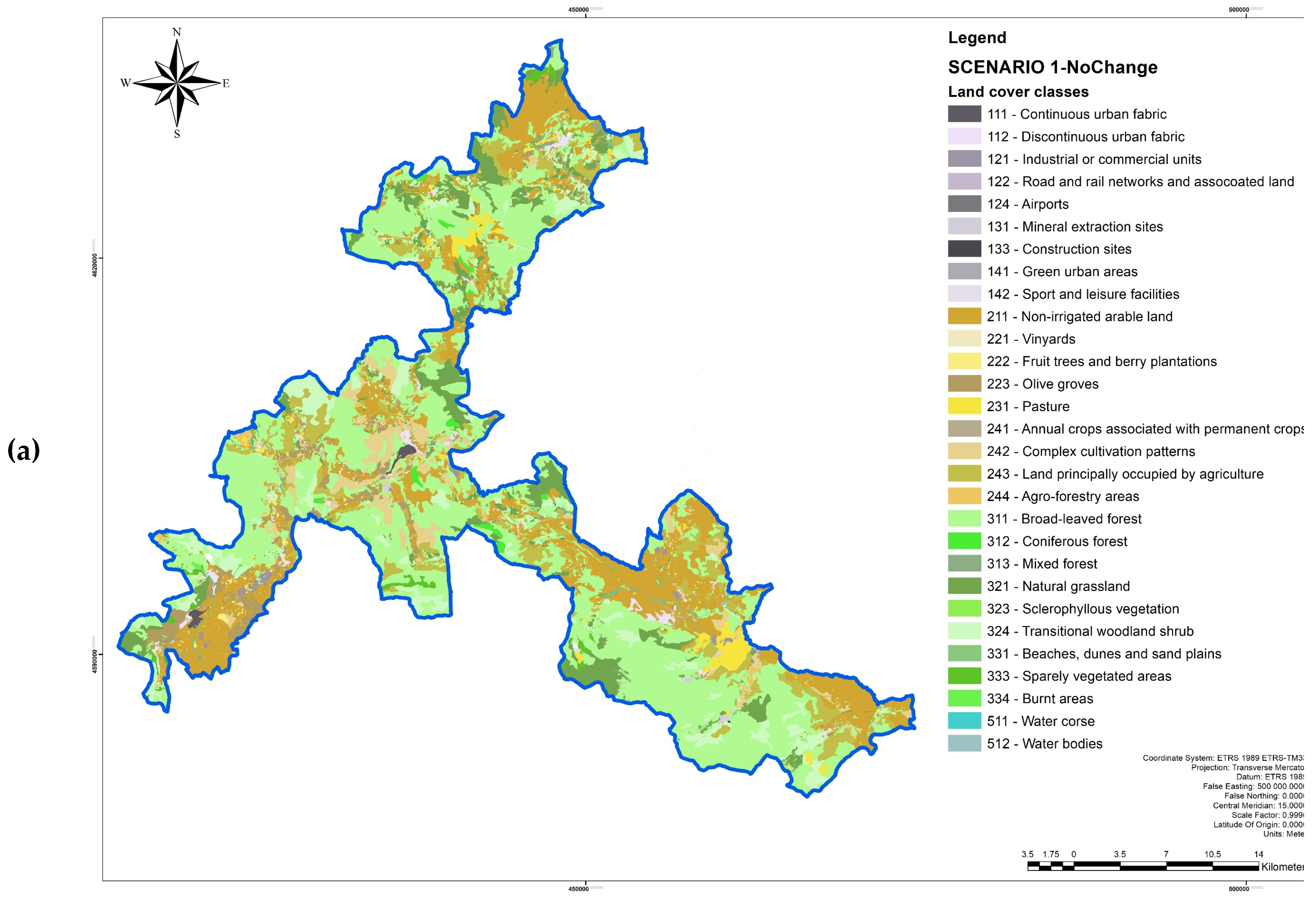
  • Scenario 1—No changes scenario: the current land uses and land covers is supposed to last for years. This scenario is based on the CLC 2018 classification, integrated with the Molise Land Use Map 2010;
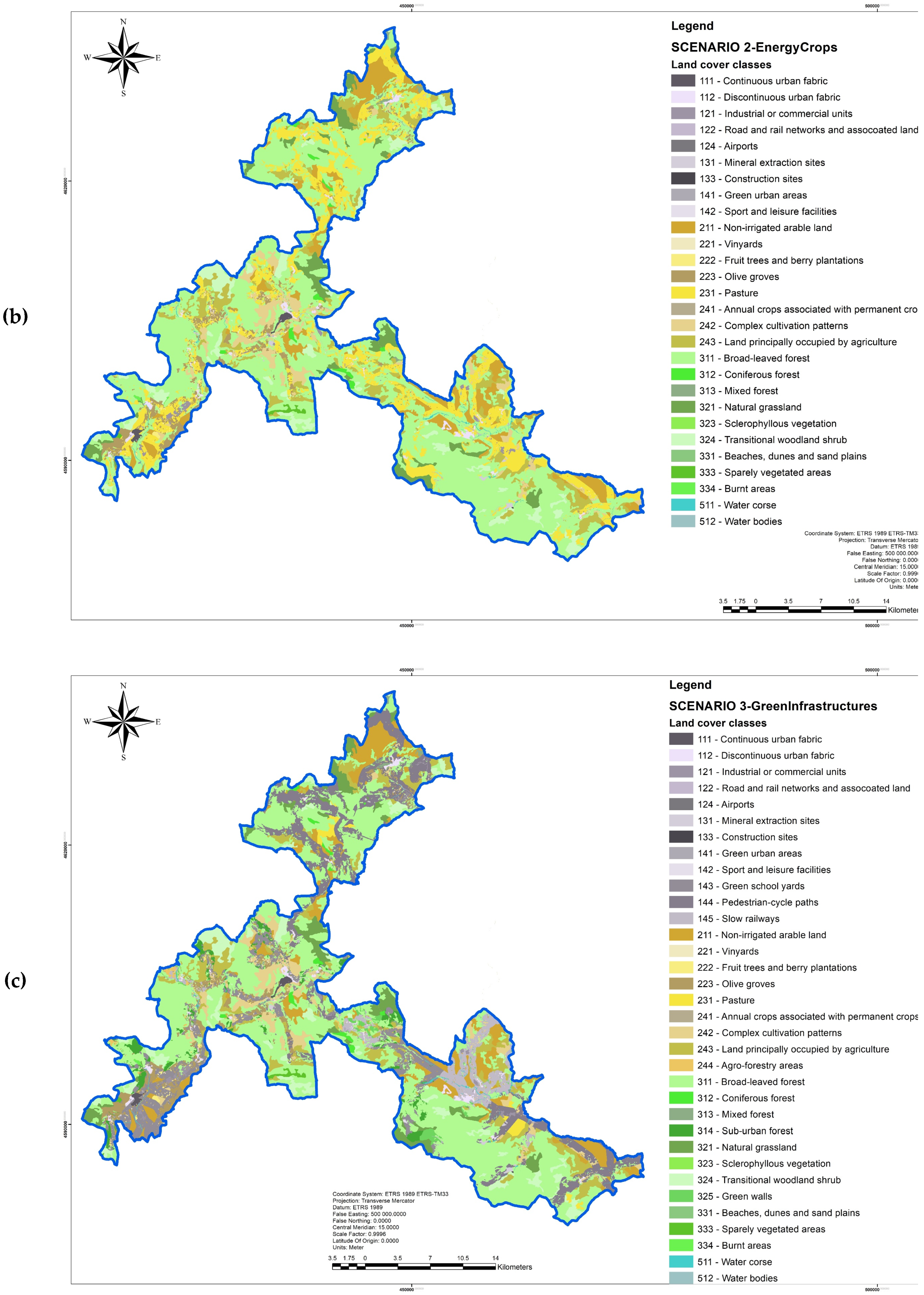
  • Scenario 2—Energy crops scenario: land-use change is allowed for some agricultural uses (arable lands, pasture, heterogeneous agricultural areas) and some forest and semi-natural areas (scrub and/or herbaceous vegetation associations and open spaces with little or no vegetation) within marginal lands into energy crops (poplar, giant reed, thistle). Specifically thistle and giant reed are assimilated to land-cover class “231—Pasture” because they are perennial grass or biennial or annual plants, that are cultivable and capable of adapting to different types of context and climate; whereas poplar is included in land-cover class “311—broad-leaved forest”, as reported by the CLC 2012 classification, 4th level (class 3116—"Broad-leaved forest—Woods of hygrophilous species").
  • Scenario 3—Green infrastructures scenario: land-use changes, within marginal lands, can be converted from semi-natural areas (composed by open space with little or no vegetation) and agricultural areas (devoted to arable lands and pasture) into green areas (such as sub-urban forest, pedestrian and cycle paths, new wetlands, green walls, green school yards, slow railways, etc.). Specifically, the new land cover classes considered are: “143—Green school yards”; “144—Pedestrian-cycle paths”; “145—Slow railways”; “314—Sub-urban forest”; “325—Green walls”.
Starting from the new landscape compositions and configurations, an environmental impacts assessment was performed by means of Ecosystem Services, focusing on the benefits people obtain from ecosystems. Starting from the first definition developed in the 1980s, there are now many classifications of ESs. The Millennium Ecosystem Assessment (MEA) [49] is considered to be a universal accepted definition, due to its “provision”, “regulation” and “support” services classifications. The importance (‘‘value’’) of ecosystems and their services can be expressed in different ways: ecological or biophysical, socio-cultural and economic. Each way is characterized by a specific assessment approach and specific theoretical postulates.
Inside ESs, Landscape metrics are important indicators, allowing for analyzing landscape pattern aspects intricately connected with ecosystem functionalities [14,67,68]. They are algorithms that quantify specific spatial characteristics of patches, classes of patches or entire landscape mosaics, or of the patch mosaic in the neighborhood of each focal cell [69]. Usually, composition and configuration are the two categories which describe the LMs: composition analysis allows quantifying landscape patterns of the map without reference to spatial attributes (i.e., the variety and abundance of patch types), while configuration analysis allows quantifying the spatial configuration of the map (i.e., the spatial character and arrangement, position or orientation of patches within the class or landscape) [69].
Landscape metrics have been extensively used in a variety of fields [70,71,72,73,74], such as biodiversity and habitat analysis, aesthetics of landscapes, evaluation of landscape patterns and changes therein and management, planning and monitoring, etc. Hundreds of landscape metrics were developed in the last three decades [75,76,77,78,79], and many of the landscape metrics are correlated to each other.
The present study focused on some LMs which deepen the fragmentation aspect of landscapes because of the importance of fragmentation issue in spatial planning policies [80] and because it is deeply connected with the land-use scenarios comparison. In Europe, landscape fragmentation has been a fairly widespread process since the end of the 19th century in intensively used regions. Fragmentation could be considered as the product of the linkage of built-up areas via linear infrastructure, such as roads and railroads [81,82]. It consists of the transformation of larger patches of habitat in smaller ones, or fragments, which tend to be more isolated than in original conditions [83]. Habitat fragmentation analysis by means of landscape metrics allows for observing a process in which contiguous habitats are progressively sub-divided into smaller, geometrically more complex areas [84].
Starting from similar studies concerning landscape fragmentation analysis, in the present work, a suite of metrics available in the FRAGSTATS ver 4 software package (University of Massachusetts, Amherst, MA, USA) [62] was selected. The class- and landscape-levels were deepened. Class-level metrics, deepening the amount and spatial distribution of a single patch type, help with understanding the fragmentation aspects. Landscape-level metrics, based on the spatial pattern of entire landscape mosaics, help with understanding the landscape heterogeneity, as a measure of the overall landscape structure.
For each landscape map (the three LUC scenarios), the metrics were computed with the raster version (GeoTIFF) of FRAGSTATS [62]. The analysis was performed for the marginal lands inside the commuting zone perimeter, to consider not only the internal conditions but also the boundary ones and the relationships with the neighborhood. The metrics are described in Table 1.
The Largest patch index (LPI) and Percentage of landscape (PLAND) belong to the “Area and Edge Metrics” metrics group that deals with the size of patches and the amount of edge created by these patches, which are useful in landscape fragmentation analysis. Although there are myriad effects of habitat fragmentation on habitat use patterns, and intra- and inter-specific interactions, many of these effects are caused by a reduction in habitat area and continuity, and an increase in the proportion of edge-influenced habitats [62].
The other metrics fall into a metrics aggregation group that refers to the tendency of patch types to be spatially aggregated (or with contagious distributions). They measure complexity, arrangements and proximity (configuration) using the composition of the landscape or abundance of certain classes within the landscape. These analyses play a crucial role in the process of habitat loss and fragmentation: habitat loss and fragmentation generally involve the disaggregation of contiguous habitat into more dispersed habitats and/or separated (i.e., subdivided) and more isolated patches [62].

3. Results

The marginal areas present a multiplicity of negative factors (economic, environmental and settlement nature factors), which together contribute to determining a low level of development; the peripheral areas with poor agriculture present a low level of agricultural productivity, due to their eccentric position with respect to the urban and infrastructural systems, rather than due to physical-environmental problems. Deepening the study area’s environmental, settlement and economic conditions, Rural Atlas allows us to identify 43 municipality territories as marginal areas, 17 as peripheral areas with poor agriculture and 1 area as a tourist and/or urban area (Figure 4b).
These areas, compared with Dir. CEE 268/75 and Italian Law n. 984/77, are completely included in the perimeter of Less favored areas (Figure 4a). The only exceptions are two municipalities bordering Venafro (the tourist and / or urban area), which are marginal areas in the elaboration of the rural Atlas, while, for the EEC Directive, they are partially delimited as mountain disadvantaged areas. Finally, population distribution and demographic trends (as performance’ indicators) analysis also shows a real correspondence with respect to depopulation phenomena (Figure 4c): 28 municipalities are classifiable as disadvantaged areas with decreasing populations, 8 municipalities are classifiable as disadvantaged areas with increasing populations, 12 as non-disadvantaged areas with decreasing populations and 13 as non-disadvantaged areas with increasing populations.
Within these contexts, the integration of results obtained by means of territories in between each approach, can contribute to a better understanding of the real physical and socio-economic conditions, and can help to define possible areas of first interventions in order to ensure there is sustainable development.
The first steps allowed for identifying possible “cities” and “urban centers” in High Molise area: 35 High density urban centers were identified, with more than 1500 inhabitants per km2, but clustering and grouping tools showed that there are no “Urban centers” within the study area. “High Molise” areas are only found in the urban center of Campobasso, which is the capital of Molise. These results highlight the marginality character—with respect to the demographic (and socio-economic) dynamics—of the context; as a result, the study of commuting and employment relationships at a regional scale is particularly interesting.
The Isernia provincial capital (and two other neighboring municipalities) presents a high level of commuting (up to 35%), but it is also possible to observe a well-defined network (with two directions, from north to south-west as well as south-east and crossing Isernia) of municipalities that are dependent, from a working point of view, on the main regional and extra-economic poles (Caserta-Rome and Campobasso-Foggia, respectively).
The resulting Commuting Zones, sort out by the inclusion/dropping of a municipality, underline the flow previously described, from the mountain areas to the main urban center of Isernia, and then along the Isernia-Campobasso route.
The defined commuting zones (Figure 5) cover 851 km2, entail 31 municipalities (with 94,576 inhabitants) and include the main local industrial centers of Venafro-Pozzillo (IS) and Bojano (CB).
Inside these areas, the maximum population analysis shows an interesting geographical continuity between the municipalities characterized by the average values of employees (according to a literature review) in the various economic sectors and by the main road axes of Campobasso-Isernia and Isernia-Venafro-Caianiello-Rome. The areas involved consist of valleys, surrounded by landscape with high naturalness values: the Matese massif (with the next Matese National Park) and the Meta Mountains (with the Abruzzo, Lazio and Molise National Park).
The final deepening involving LULC types allows for defining the in-between territories in the High Molise area, which are 354.5 km2. Specifically, two types of TiBs are recognizable:
  • disadvantaged mountain or hilly areas, with low levels of agricultural productivity, with a decreasing population, in the north of the study area and, to a small extent, in the easternmost area (144 km2);
  • partially mountainous, non-disadvantaged areas, with a population that is mostly growing, in the south-east and south-west of the study area (210.5 km2).
In the present paper, these locations are defined as marginal lands, and cover 19.5% of the total study area.
Artificial surfaces cover 6.8 km2 of the total study area, agricultural areas cover 176.4 km2, forest and semi-natural areas cover 168.2 km2 and water bodies cover 2.9 km2. For the agricultural areas, arable lands cover 66.4% and permanent crops cover 14.4%. For the forest and semi-natural areas, forest areas cover 58.8% and the scrub and/or herbaceous vegetation associations cover 38.1%.
The marginal lands identification in the High Molise region allowed for a scenario building phase and a consequent environmental assessment.
Three scenarios were built. Figure 6a–c, Figure 7a,b and Table 2 show the spatial configurations and the areas for each land-use class.
In scenario 2, the classes “211—Non-irrigated arable land”, “321—Natural grassland”, “324-Transitional woodland shrub” and “333-Sparely vegetated areas” decrease their whole area by 56%, while the classes “231–Pasture” and “311—Broad-leaved forest” increase, respectively, by 570% and 20%.
In scenario 3, the classes “14—Artificial, non-agricultural vegetated areas” increase, overall, of 230% and class “31—Forest” increase of 0.1%, at the expense of “231—Pasture”, “244—Agri-forestry areas”, “321—Natural grassland”, “324 - Transitional woodland shrub” and “333 - Sparely vegetated areas”.
Landscape metrics analysis was performed at class and landscape levels for the three scenarios.
At a class level, PLAND and LPI indices show substantially overlapping trends (Figure 8a,b) and reveal a similar pattern of small patches connected to artificial surfaces and water bodies classes where high values are mainly in some natural and semi-natural contexts and in some agricultural areas:
  • Scenario 1 shows higher values (in terms of presence and dimensions) for those classes which characterize the landscape marginality: 211—Non irrigated arable lands, 321—Natural grassland and 324—Transitional woodland shrub;
  • Scenario 2 shows the new predominance of the classes related to the new energy crops (231—Pasture and 311—Broad leaved forest);
  • Scenario 3 presents high values for the forest and semi-natural classes (311—Broad leaved forest) and, unlike the other 2 scenarios, for the artificial surfaces connected with the recreation functions (14—Artificial, non-agricultural vegetated areas). The 231—Pasture, 321—Natural grassland and 324—Transitional woodland shrub classes increase the size gap (in terms of decreasing) with other scenarios.
Both LSI and PD (Figure 8c,d) suggest that some agricultural areas (241—annual crops associated with permanent crops and 244—agro-forestry areas) have the most fragmented landscape with moderate vegetation cover. Instead, the less fragmentated classes are the following: the non-irrigated arable land and the herbaceous vegetation associations in scenario 1; pasture and forest areas in scenario 2; forest and new urban green areas in scenario 3.
The patterns indicated by the Aggregation Index (Figure 8e) show high aggregation levels (on average always above 90%) for all land-use classes, in scenarios 1 and 3. In scenario 2, the agroforestry areas show significant disaggregation. Classes of artificial surfaces connected with new recreation functions and the sub-urban forest have low aggregation index values, due to their introduction only in specific scenarios.
At the landscape level (Figure 8f), PD and LPI show less fragmentation risk connected with land-use change scenarios due to the lower density index (−15% and −4%, respectively, in scenarios 2 and 3), and to the increasing in size values by an average of 13%. Also, the LSI metric follows this trend, with a respective decreasing in values for new scenarios of (−)8% and (−)3%. The AI is not particularly useful at a landscape level, while the CONTAG metric shows different trends in scenario 2 and 3: while the values increase by 2% in scenario 3, there is a 5% decrease in scenario 2, depending on the introduction of new land-use classes related to recreation in urban areas.

4. Discussion

4.1. The Identification of Marginal Lands

The disadvantaged and marginal areas issue is increasingly becoming a subject of focus for the scientific literature, as well as for numerous legislative and regulatory provisions [28].
The study proposes, as a first step, the integration of different approaches for the identification of marginal lands in Southern Italy. The paper refers to the scientific debate on marginal lands, starting from the first definitions with predominantly negative nature that are linked to disadvantageous conditions to remedy the most recent definitions referable to the concepts of hybrid landscape or middle lands, which take into account the "in transformation" character of these contexts. Marginal lands can therefore be considered as resources too, new engines of development for larger regions.
The knowledge process was reflected in a framework building for landscape analysis aimed at identifying current marginal lands. The proposed framework provides for the integration of two approaches, emblematic of the two meanings (in only negative and positive terms): the Less Favored Areas (LFAs) and the Territories in Between (TiBs). The methodology allows for highlighting critical issues and, at the same time, indicates development opportunities. Socio-economic conditions, location factors and morphological characteristics have been the basis for land-use change scenarios building.
The results showed marginality conditions for about 20% of the entire study area. These territories branch off along the Foggia–Isernia and Rome–Isernia–Adriatic Sea road lines and are characterized by very different characteristics:
  • The Rome–Isernia line presents territories that can be considered to be evolving, are not morphologically disadvantaged, have a growing population and contain economic activities among the most developed in the Molise region, but still not fully developed.
  • The Isernia–Adriatic Sea line, on the other hand, presents conditions of morphological and socio–economic disadvantage. It consists of mountain areas with low population levels and few economic activities, but with elevated levels of environmental quality, underlined by the presence of SCIs and SPAs and a National Park.
  • The Isernia–Foggia line has a mixed character, with: non–disadvantaged sub–areas and an increasing population (mainly the territories bordering Isernia); sub-areas with physical and socio-economic conditions of disadvantage, but with high levels of environmental quality, highlighted by the presence of SCIs, SPAs and one Regional Park; sub-areas with not disadvantaged morphological conditions, but with negative demographic trends and economically disadvantaged conditions.
The awareness of so different conditions leads to different solutions in scenarios building processes.
Within marginal lands, areas with low profitability crops, with little or no vegetation, that are closest to urban centers and road axes or—still—have a high environmental value, were considered to be the most susceptible areas to land-use change in the short–medium term for economic reasons (on one hand due to low acquisition costs, on the other, due to tourism opportunities) or social reasons (on one hand due to abandonment or under-utilization, on the other, due to recreation opportunities) or logistics (linear infrastructure realizations). According to development prospects suggested by EU directives, three scenarios were built:
  • The no-change status, with the permanence of current environmental conditions and socio-economic driving forces;
  • the development of a bio-energy chain, with poplar, thistle and giant reed crops;
  • the implementation of a green infrastructures network, as an improvement to the quality of local life and as development engine for the tourism sector.
As a result of anthropic activities, the landscape is becoming increasingly complex (in its structure, in the functions distribution, in ways of being perceived). This complexity translates into new landscape definitions and classifications and new meanings, which help to understand its distinctive characteristics; this means new intervention strategies are necessary.
Landscape analysis in support of the government, planning and management processes must include this complexity. The present work, in the middle of a scientific and government debate on the definition and identification of marginal lands, intends to provide a support framework for territorial analysis. The goal is not just a simple analysis application but is to support and guide the prognosis and territorial policies phases in the planning process, focusing on the resources and critical issues which emerge. Marginal lands become the areas from which to start which are areas of priority for intervention within the strategic landscape planning and with a long-term vision, to trigger transformation processes spread over wider territories.
The framework, which is largely linked to approaches already developed in the scientific field and used from a practical-operational point of view, has the potential to deal with the topic in a more complex way. In the present case, the application of the only approach through LFA, would have led to the recognition of disadvantageous conditions on almost the entire study area, without allowing for focusing attention on specific areas (in terms of resources or critical issues), from which to start for strategies and intervention policies. The application of only the TiB approach would have led to the identification of specific and defined areas, with precise socio-economic and infrastructural characteristics, without an overview of the context in which they are inserted. The critical integration of the two methodologies instead allowed a detailed analysis of the coarse-scale landscape and, at the same time, allowed us to identify focus-areas in terms of resources or critical issues on which to concentrate first intervention strategies.

4.2. The Environmental Impacts Assessment

The supposed scenarios involve changes in landscape composition, structure and function. Habitat loss and fragmentation are increasingly recognized as the prevailing by-product of anthropic activity in landscapes, and as a major cause of declining biodiversity [62,83,85]. For this reason, in order to hypothesize the possible impacts associated with supposed land-use change, a specific analysis of landscape fragmentation risk was performed using an ecosystem services approach and landscape metrics, which is considered to be one of the hot topics of modern landscape ecological research [79].
In the present work, the Fragstat landscape metrics were preferred due to their worldwide application for similar case studies, allowing us to contribute in the scientific debate about hybrid geographies individuation and the impacts of current driving forces on the landscape. At the same time, starting from the most common metrics described here, devoted to regional scale application and in the strategic planning phase, additional ones could be developed and tested on target contexts in order to highlight specificity and particularity, and to contribute in a more effective way to the landscape planning process at a local scale. Based on this assumption, the selected metrics demonstrated good repercussions / impacts of the land-use change on the landscape, in terms of fragmentation.
Scenario 2 is the most preferable scenario according to the Largest patch index (LPI), Percentage of landscape (PLAND), Patch density (PD), Landscape shape index (LSI) metrics (Scenario 1, the actual state, or no-change, is the worst scenario). Largest patch index (LPI) (both at class and landscape levels) and Percentage of landscape (PLAND) (at the class level), show a possible decrease of landscape fragmentation, as result of the increase in the percentage of total landscape area comprised by the forest patches and the pasture ones, i.e., by those habitats considered to be very important in terms of habitat quality services and biodiversity. Also, the PD (at the class and landscape levels) highlights a reduced fragmentation risk in Scenario 2, thanks to its coarse-grain texture and thanks to the prevalence of specific classes related to new land uses. Through LSI analysis, at the landscape level, the greatest geometric complexity is shown by Scenario 1 (the worst) and Scenario 3. At the class level, parallel to the other metrics described, the semi-natural areas with little or no vegetation and the agroforestry areas are the habitats that benefit from Scenario 3 and, above all, from Scenario 2.
Scenario 3 is the preferable one, according to Aggregation index (AI) and Contagion (CONTAG) metrics. At the landscape level, the AI metric highlights higher aggregation levels in Scenarios 2 and 3. At the class level, both AI and CONTAG prefer Scenario 3, thanks to less intermixing of units of different patch types under this scenario. It should be emphasized, however, that Scenarios 1 and 2 suffer from the fact that some classes attributable to green infrastructures have not been included in the assessment.
The LM analysis contributed significantly to the present study, allowing for deepening the risk of fragmentation connected with land-use change scenarios. This aspect is an important reference for landscape planning and management policies, because it is closely correlated with the greater functional quality of landscape [86], which is the basis not only for habitat quality services, but also for all the other services (from the amenity and recreation ones to the air quality regulation services or to the food and goods supply). The positive results obtained, in addition to suggesting hypotheses for the study-area development, can be read as a validation of the proposed framework for the identification of marginal lands and for the land-use scenarios building. The aim is to provide, with respect to and enhancement of the high levels of environmental quality, landscape planning support for the socio-economic development and alternatives, both in terms of energy crops and green infrastructures. The impacts analyzed, however, are still very limited. More extended analyses will be necessary, concerning both socio-economic driving forces and environmental aspects, to support development policies in the High Molise region.

5. Conclusions

The proposed method integrates a different land-use and landscape planning approach (in landscape analysis and environmental impacts assessment fields), in order to support decision maker actions, based on a transparent and sharing process, supported by scientific studies and targets towards a new hybrid landscape which needs new and specific approaches.
Currently, ordinary landscape and land-use planning is lacking in specific tools calibrated for marginal lands: the only efforts in this area are often oriented to provide (economic) support tools for territories that are seen only in negative terms and not for the great potential they have. Strategic environmental assessment is a tool that certainly complements ordinary planning, but it is not fully utilized very often. This work therefore forms part of the scientific and government debate on the matter, with the aim of stimulating a greater knowledge of marginal areas and a consequent greater awareness of their current and potential uses.
The developed methodology should not simply provide relief for marginal conditions or to be used as a simple analysis application. It also should be used for critical assessment of possible forms of landscape development, identifying and recognizing the critical features to be remedied and the valuable characteristics that can be enhanced or simply preserved. The marginal lands become engines of development and resources for a whole region in the context of sustainability that is not only environmental but also socio-cultural, connected to new economic forms.
The paper framework aims to integrate an ES indicators assessment into the most common and shared landscape planning techniques, starting from the analysis of marginality criteria and using studies which deepened this relationship [50,87,88,89]. The proposed methodology shows the advantages of: (i) conducting a preliminary but target analysis on specific characteristics of a landscape, raising the issue of the need for socio-economic development together with preserving local environmental resources; (ii) deepening and relating the marginal conditions with the risk of fragmentation associated with any intervention proposals for the development of marginal lands.
At the same time, in order to improve the important gaps linked to detail of information, any integration of aspects, stakeholder participation, likelihood of hypotheses and upcoming developments of the project may be able:
  • to deepen the parameters / factors selection in marginal lands identification, in order to integrate the main factors with other ones which can contribute to defining problem areas;
  • to analyze aspects like profitability and intensity usability of territories or current land-use planning zoning rules, in order to build more reliable and realistic land-use scenarios;
  • to perform landscape analysis by means of satellite images at a local scale, in order to obtain land cover maps that are more updated and precise (which is useful and necessary for land patterns analysis) and to calibrate interventions and projects that are more relevant for a specific context. In this way, it will be possible to overcome the current limits of using Corine Land Cover maps due to the scarce levels of coarse detail by improving the overall quality of metric analysis results.
  • to integrate simulations / assessments expected on different ecosystem services, in order to have a more articulated and responsive analyses/simulations of the possible impacts from LUC;
  • to simulate costs of carrying out the interventions, in order to compare the investments in targeted areas with their expected environmental impacts/benefits.
Marginal areas identification can therefore, potentially, provide a strategic element to support decision makers in order to define sustainable development policies for both local people rights and environmental preservation points of view, to use local resources (abandoned areas for agricultural uses, availability of manpower, know-how of cultivation practices) and to evaluate development alternatives that guarantee higher incomes and interest in the sector.
In these terms, the present study can be a reference for the analysis and planning of other contexts, characterized by new conditions of marginality that can be physical, functional or perceptual, which very often also present enormous development opportunities or have high values of environmental quality to be preserved.

Author Contributions

Conceptualization, E.C. and S.P.; methodology, E.C.; data curation, E.C.; writing—original draft preparation, E.C.; writing—review and editing, E.C., E.S.d.P. and S.P.; supervision, S.P.; funding acquisition, E.C. and S.P. All authors have read and agreed to the published version of the manuscript.

Funding

This research was funded by the Rural Development Program for 2014–2020 of Campania Region Project RiAGRI-Sele (assigned to S.P), with the help of the research agreement between Vesuvius National Park and the Department of Agricultural Sciences of 2018 (assigned to E.C. and S.P.) and of FFABR—Funding for Basic Activities Related to Research 2017 (MIUR), which was assigned to S.P.

Acknowledgments

This paper considers some of the knowledge of the CAMPANIA TRASPARENTE Project.

Conflicts of Interest

The authors declare no conflict of interest.

References

  1. Ode, Å.; Hagerhall, C.M.; Sang, N. Analysing visual landscape complexity: Theory and application. Landsc. Res. 2010, 35, 111–131. [Google Scholar] [CrossRef]
  2. Wandl, D.A.; Nadin, V.; Zonneveld, W.; Rooij, R. Beyond urban–rural classifications: Characterising and mapping territories-in-between across Europe. Lands. Urban Plan. 2014, 130, 50–63. [Google Scholar] [CrossRef]
  3. Wandl, A.; Balz, V.; Qu, L.; Furlan, C.; Arciniegas, G.; Hackauf, U. The circular economy concept in design education: Enhancing understanding and innovation by means of situated learning. Urban Plan. 2019, 4, 63–75. [Google Scholar] [CrossRef]
  4. Frijters, E. Tussenland; Nai Uitgevers: Rotterdam, The Netherlands, 2004. [Google Scholar]
  5. Secchi, B. La Periferia; Casabella: Milan, Italy, 1991; p. 583. [Google Scholar]
  6. Webber, M.M. The joys of spread-city. Urban Design Int. 1998, 3, 201–206. [Google Scholar] [CrossRef]
  7. Andexlinger, W. TirolCity; Folio Verlag: Vienna, Austria, 2005. [Google Scholar]
  8. Mosey, G.; Heimiller, D.; Dahle, D.; Vimmerstedt, L.; Brady-Sabeff, L. Converting Limbo Lands to Energy-Generating Stations: Renewable Energy Technologies on Underused, Formerly Contaminated Sites; No. EPA/600/R-08-023, NREL/TP-640-41522; Nat. Renew. Energy Lab.(NREL): Golden, CO, USA, 2007. Available online: https://www.nrel.gov/docs/fy08osti/41522.pdf (accessed on 28 June 2020).
  9. Newton, G.A.; Claassen, V.P. Rehabilitation of Disturbed Lands in California: A Manual FOR Decision-Making; Geological Survey: Sacramento, CA, USA, 2003. Available online: https://www.conservation.ca.gov/omr/reclamation/Documents/sp123.pdf (accessed on 28 June 2020).
  10. Zumkehr, A.; Campbell, E.; Historical, U.S. Cropland Areas and the Potential for Bioenergy Production on Abandoned Croplands. Environ. Sci. Technol. 2013, 47, 3840–3847. [Google Scholar] [CrossRef]
  11. U.S. Environmental Protection Agency. Landfill Methane Outreach Program. Available online: https://www.epa.gov/lmop (accessed on 1 May 2020).
  12. Fuchs, C. UN Convention to Combat Desertification: Recent Developments. In Max Planck Yearbook of United Nations Law; Oxford University Press: Oxford, UK, 2008; Volume 12, pp. 287–300. Available online: https://pdfs.semanticscholar.org/1c87/462acf80fc9aa4843837a744c6f8041c24d8.pdf (accessed on 28 June 2020).
  13. Milbrandt, A.R.; Heimiller, D.M.; Perry, A.D.; Field, C.B. Renewable energy potential on marginal lands in the United States. Renew. Sustain. Energy Rev. 2014, 29, 473–481. [Google Scholar] [CrossRef]
  14. Cervelli, E.; di Perta, E.S.; Pindozzi, S. Energy crops in marginal areas: Scenario-based assessment through ecosystem services, as support to sustainable development. Ecol. Indic. 2020, 113, 106180. [Google Scholar] [CrossRef]
  15. Directive, Council. 75/268/EEC of 28 April 1975 on Mountain and Hill Farming and Farming in Certain Less-Favoured Areas. Official Journal of the European Union. 1975. Available online: https://op.europa.eu/en/publication-detail/-/publication/86e63262-05ec-4633-94bd-9226dc1b094a/language-mt (accessed on 1 May 2020).
  16. Council Regulation (EC) No 950/97 on Improving the Efficiency of Agricultural Structures. Official Journal of the European Union. Available online: https://eur-lex.europa.eu/legal-content/en/TXT/?uri=CELEX%3A32005R1698 (accessed on 1 May 2020).
  17. Council Regulation (EC) No 1257/1999 of 17 May 1999 on support for rural development from the European Agricultural Guidance and Guarantee Fund (EAGGF) and amending and repealing certain Regulations. Official Journal of the European Union. Available online: https://eur-lex.europa.eu/legal-content/EN/TXT/PDF/?uri=CELEX:31999R1257 (accessed on 1 May 2020).
  18. Council Regulation (EC) No 1698/2005 of 20 September 2005 on support for rural development by the European Agricultural Fund for Rural Development (EAFRD). Official Journal of the European Union. Available online: https://eur-lex.europa.eu/LexUriServ/LexUriServ.do?uri=OJ:L:2005:277:0001:0040:EN:PDF (accessed on 1 May 2020).
  19. MacDonald, D.; Crabtree, J.R.; Wiesinger, G.; Dax, T.; Stamou, N.; Fleury, P.; Gibon, A. Agricultural abandonment in mountain areas of Europe: Environmental consequences and policy response. J. Environ. Manag. 2000, 59.1, 47–69. [Google Scholar] [CrossRef]
  20. Dwyer, J.; Clark, M.; Kirwan, J.; Kambites, C.; Lewis, N.; Molnarova, A.; Bolli, M. Review of Rural Development Instruments: DG Agri project 2006-G4-10; Final Report; 2008; Available online: https://mpra.ub.uni-muenchen.de/50290/ (accessed on 1 May 2020).
  21. Storti, D.; Zumpano, C.; Mantino, F.; Murano, R.; Cesaro, L.; Monteleone, A.; Ascione, E. Le Politiche Comunitarie per lo Sviluppo Rurale; Rapporto 2008/2009: Il quadro degli interventi in Italia: 2010. Istituto Nazionale di Economia Agraria; Available online: http://156.54.184.84/bitstream/inea/528/1/Politiche_Comunitarie_2008-2009.pdf (accessed on 1 May 2020).
  22. Dijkstra, L.; Poelman, H. Cities in Europe: The new OECD-EC definition. Reg. Focus 2012, 1, 1–13. [Google Scholar]
  23. Eurostat Regional Yearbook 2018 Edition; Publications Office of the European Union: Luxembourg, 2018; Available online: http://ec.europa.eu/eurostat/ (accessed on 28 June 2020).
  24. Taelman, S.E.; Tonini, D.; Wandl, A.; Dewulf, J. A holistic sustainability framework for waste management in European cities: Concept development. Sustainability 2018, 10, 2184. [Google Scholar] [CrossRef] [Green Version]
  25. Tilman, D.; Hill, J.; Lehman, C. Carbon-negative biofuels from low-input high-diversity grassland biomass. Science 2006, 314, 1598–1600. [Google Scholar] [CrossRef] [PubMed] [Green Version]
  26. Food and Agriculture Organization of the United Nations (FAO). Declaration of the High-level Conference on World Food Security: The Challenges of Climate Change and Bioenergy; FAO Newsroom: Rome, Italy, 2008; Published online. [Google Scholar]
  27. Robertson, G.P.; Dale, V.H.; Doering, O.C.; Hamburg, S.P.; Melillo, J.M.; Wander; M.M. Sustainable biofuels redux. Science 2008, 322, 49–50. [Google Scholar] [CrossRef]
  28. Kang, S.; Post, W.M.; Nichols, J.A.; Wang, D.; West, T.O.; Bandaru, V.; Izaurralde, R.C. Marginal lands: Concept, assessment and management. J. Agric. Sci. 2013, 5, 129. [Google Scholar] [CrossRef] [Green Version]
  29. EU COM (2011) 244 The EU Biodiversity Strategy to 2020. Communication From The Commission To The European Parliament, The Council, The Economic And Social Committee And The Committee Of The Regions Our Life Insurance, Our Natural Capital: An Eu Biodiversity Strategy To 2020 Communication From The Commission To The European Parliament, The Council, The Economic And Social Committee And The Committee Of The Regions Our Life Insurance, Our Natural Capital: An EU Biodiversity Strategy to 2020. Available online: http://ec.europa.eu/environment/nature/biodiversity/comm2006/2020.htm (accessed on 1 May 2020).
  30. EEA. Tech18-2011. European Green Infrastructure Strategy-Green Infrastructure and Rural Abandonment. Available online: https://www.eea.europa.eu/publications/green-infrastructure-and-territorial-cohesion (accessed on 1 May 2020).
  31. EU COM/2013/0249 final-Communication from the commission to the European parliament, the council, the European Economic and Social Committee and the Committee of the Regions Green Infrastructure (GI)—Enhancing Europe’s Natural Capital. Brussels. Available online: https://ec.europa.eu/environment/nature/ecosystems/docs/green_infrastructures/1_EN_ACT_part1_v5.pdf (accessed on 1 May 2020).
  32. IMESLP-Italian Ministry of Environment, Sea and Land Protection. In Proceedings of the Green Infrastructures and Ecosystems Services as Instruments for Environmental Policy and Green Economy: Potentiality, Criticality and Recommendations, Rome, Ital, 11–12 December 2013. Available online: http://www.minambiente.it/sites/default/files/archivio/allegati/natura_italia/natura_italia_documento_sintesi_finale_eng.pdf (accessed on 1 May 2020).
  33. EC-Directive 2009/28/EC of the European Parliament and of the Council of 23 April 2009 on the promotion of the use of energy from renewable sources and amending and subsequently repealing Directives 2001/77/EC and 2003/30/EC. Available online: https://eur-lex.europa.eu/LexUriServ/LexUriServ.do?uri=OJ:L:2009:140:0016:0062:EN:PDF (accessed on 1 May 2020).
  34. EU-Directive 2018/2001 of the European Parliament and of the Council of 11 December 2018 on the promotion of the use of energy from renewable sources. Document 32018L2001. Available online: https://eur-lex.europa.eu/legal-content/EN/TXT/?uri=uriserv:OJ.L_.2018.328.01.0082.01.ENG (accessed on 1 May 2020).
  35. Lal, R. Beyond Copenhagen: Mitigating climate change and achieving food security through soil carbon sequestration. Food Secur. 2010, 2, 169–177. [Google Scholar] [CrossRef]
  36. Tilman, D.; Socolow, R.; Foley, J.A.; Hill, J.; Larson, E.; Lynd, L.; Williams, R. Beneficial biofuels—the food, energy, and environment trilemma. Science 2009, 325, 270–271. [Google Scholar] [CrossRef] [PubMed] [Green Version]
  37. Godet, M. Introduction to la prospective: Seven key ideas and one scenario method. Futures 1986, 18, 134–157. [Google Scholar] [CrossRef]
  38. Schwartz, P. The Art of the Long View: Planning for the Future in An Uncertain World; Currency Doubleday: New York, NY, USA, 1996; p. 258. [Google Scholar]
  39. Mietzner, D.; Reger, G. Advantages and disadvantages of scenario approaches for strategic foresight. Int. J. Technol. Intell. Plan. 2005, 1, 220–239. [Google Scholar] [CrossRef] [Green Version]
  40. Malczewski, J. GIS-based multicriteria decision analysis: A survey of the literature. Int. J. Geogr. Inform. Sci. 2006, 20, 703–726. [Google Scholar] [CrossRef]
  41. Verburg, P.H.; Overmars, K.P. Combining top-down and bottom-up dynamics in land use modeling: Exploring the future of abandoned farmlands in Europe with the Dyna-CLUE model. Lands. Ecol. 2009, 24, 1167. [Google Scholar] [CrossRef]
  42. Amer, M.; Tugrul, U.D.; Antonie, J. A review of scenario planning. Futures 2013, 46, 23–40. [Google Scholar] [CrossRef]
  43. Houet, T.; Marchadier, C.; Bretagne, G.; Moine, M.P.; Aguejdad, R.; Viguie, V.; Masson, V. Combining narratives and modelling approaches to simulate fine scale and long-term urban growth scenarios for climate adaptation. Environ. Model. Softw. 2016, 86, 1–13. [Google Scholar] [CrossRef]
  44. Strijker, D. Marginal lands in Europe—causes of decline. Basic Appl. Ecol. 2005, 6, 99–106. [Google Scholar] [CrossRef]
  45. IPCC. Change, Intergovernmental Panel on Climate. In Climate change 2007: The Physical Science Basis: Summary for Policymakers; IPCC: Geneva, Switzerland, 2007. [Google Scholar]
  46. Searchinger, T.; Heimlich, R.; Houghton, R.A.; Dong, F.; Elobeid, A.; Fabiosa, J.; Yu, T.H. Use of US croplands for biofuels increases greenhouse gases through emissions from land-use change. Science 2008, 319, 1238–1240. [Google Scholar] [CrossRef] [PubMed]
  47. Fischer, G.; Hizsnyik, E.; Prieler, S.; Shah, M.; van Velthuizen, H.T. Biofuels and Food Security; Printed in Austria by Stiepan Druck GmbH; 2009; Available online: http://pure.iiasa.ac.at/id/eprint/8969/1/XO-09-102.pdf (accessed on 1 May 2020).
  48. MEA-Millenium Ecosystem Assessment. Ecosystems and Human Well-Being: A Framework for Assessment; Island Press: Washington, DC, USA, 2003. [Google Scholar]
  49. MEA Millenium Ecosystem Assessment. Ecosystems and Human Well-Being: Wetlands and Water; World Resources Institute: Washington, DC, USA, 2005. [Google Scholar]
  50. Albert, C.; Galler, C.; Hermes, J.; Neuendorf, F.; Von Haaren, C.; Lovett, A. Applying ecosystem services indicators in landscape planning and management: The ES-in-Planning framework. Ecol. Indic. 2016, 61, 100–113. [Google Scholar] [CrossRef]
  51. TEEB. The Economics of Ecosystems and Biodiversity: Ecological and Economic Foundations; Kumar, P., Ed.; Earthscan: London, UK; Washington, DC, USA, 2010; p. 456. [Google Scholar]
  52. Maes, J.; Teller, A.; Erhard, M.; Murphy, P.; Paracchini, M.L.; Barredo, J.I.; Meiner, A. Mapping and Assessment of Ecosystems and Their Services: Indicators for Ecosystem Assessments Under Action 5 of the EU Biodiversity Strategy to 2020; Publications Office of the European Union: Luxembourg, 2014; Available online: https://research.utwente.nl/en/publications/mapping-and-assessment-of-ecosystems-and-their-services-indicator (accessed on 1 May 2020).
  53. Cervelli, E.; Pindozzi, S.; Capolupo, A.; Okello, C.; Rigillo, M.; Boccia, L. Ecosystem services and bioremediation of polluted areas. Ecol. Eng. 2016, 87, 139–149. [Google Scholar] [CrossRef]
  54. Cervelli, E.; Pindozzi, S.; Sacchi, M.; Capolupo, A.; Cialdea, D.; Rigillo, M.; Boccia, L. Supporting land use change assessment through Ecosystem Services and Wildlife Indexes. Land Use Policy 2017, 65, 249–265. [Google Scholar] [CrossRef]
  55. La Notte, A.; D’Amato, D.; Mäkinen, H.; Paracchini, M.L.; Liquete, C.; Egoh, B.; Crossman, N.D. Ecosystem services classification: A systems ecology perspective of the cascade framework. Ecol. Indic. 2017, 74, 392–402. [Google Scholar] [CrossRef]
  56. Liu, Y.; Li, J.; Zhang, H. An ecosystem service valuation of land use change in Taiyuan City, China. Ecol. Model. 2012, 225, 127–132. [Google Scholar] [CrossRef]
  57. La Notte, A.; Maes, J.; Grizzetti, B.; Bouraoui, F.; Zulian, G. Spatially explicit monetary valuation of water purification services in the Mediterranean bio-geographical region. Int. J. Biodivers. Sci. Ecosyst. Serv. Manag. 2012, 8, 26–34. [Google Scholar] [CrossRef] [Green Version]
  58. Bateman, I.J.; Mace, G.M.; Fezzi, C.; Atkinson, G.; Turner, R.K. Economic analysis for ecosystem service assessments. In Valuing Ecosystem Services; Edward Elgar Publishing: Cheltenham, UK, 2014. [Google Scholar]
  59. Smeets, E.; Weterings, R. Environmental Indicators: Typology and Overview; European Environment Agency: Copenhagen, Denmark, 1999. [Google Scholar]
  60. Tscherning, K.; Helming, K.; Krippner, B.; Sieber, S.; Paloma, S.G. Does research applying the DPSIR framework support decision making? Land Use Policy 2012, 29, 102–110. [Google Scholar] [CrossRef]
  61. Ducci, D.; Albanese, S.; Boccia, L.; Celentano, E.; Cervelli, E.; Corniello, A.; Lima, A. An integrated approach for the environmental characterization of a wide potentially contaminated area in Southern Italy. Int. J. Environ. Res. Public Health 2017, 14, 693. [Google Scholar] [CrossRef] [PubMed] [Green Version]
  62. McGarigal, K.; Cushman, S.A.; Ene, E. FRAGSTATS v4: Spatial Pattern Analysis Program for Categorical and Continuous Maps; Computer Software Program Produced by the Authors at the University of Massachusetts: Amherst, MA, USA, 2012; Available online: http://www.umass.edu/landeco/research/fragstats/fragstats.html (accessed on 1 May 2020).
  63. Mipaaf, Ministry of Agricultural, Food and Forestry policies. Atlante Nazionale del territorio rurale. In Monografie Regionali Sulla Geografia Delle Aree Svantaggiate; Regione MOLISE, Caire Urbanistica; Available online: https://www.reterurale.it/atlante/molise/pdf/pdf_monografia/s_monografia_molise.pdf (accessed on 1 May 2020).
  64. ISTAT. National Institute of Statistics. In 15 ISTAT Census Data on Population; 2011; Available online: https://www.istat.it/en/archive/196131 (accessed on 1 May 2020).
  65. ISTAT. National Institute of Statistics. In 6 ISTAT Census Data on Economic Activities: Agriculture and Services and Industries; 2010; Available online: http://censimentoagricoltura.istat.it/ (accessed on 1 May 2020).
  66. Wandl, A. Developing a Framework to compare the performance of Territories-in-between across Europe: Defining a set of sustainability indicators. In Proceedings of the Urbanism & urbanisation VI International PhD Seminar-The Next Urban Question: Themes, Approaches, Tools, Venice, Italy, 27–29 October 2011; Universita IUAV di Venezia: Venice, Italy, 2011. [Google Scholar]
  67. Cardille, J.A.; Turner, M.G. Understanding landscape metrics. In Learning Landscape Ecology; Springer: New York, NY, USA, 2017; pp. 45–63. [Google Scholar]
  68. Frank, S.; Walz, U. 3.6. Landscape metrics. Mapp. Ecosyst. Serv. 2017, 81–86. [Google Scholar]
  69. McGarigal, K. Landscape Pattern Metrics; Wiley Online Library, Wiley StatsRef: Statistics Reference Online; 2014; Available online: https://doi.org/10.1002/9781118445112.stat07723 (accessed on 1 May 2020).
  70. Lausch, A.; Herzog, F. Applicability of landscape metrics for the monitoring of landscape change: Issues of scale, resolution and interpretability. Ecol. Indic. 2002, 2, 3–15. [Google Scholar] [CrossRef]
  71. Ji, W.; Ma, J.; Twibell, R.W.; Underhill, K. Characterizing urban sprawl using multi-stage remote sensing images and landscape metrics. Comput. Environ. Urban Syst. 2006, 30, 861–879. [Google Scholar] [CrossRef]
  72. Peng, J.; Wang, Y.; Zhang, Y.; Wu, J.; Li, W.; Li, Y. Evaluating the effectiveness of landscape metrics in quantifying spatial patterns. Ecol. Indic. 2010, 10, 217–223. [Google Scholar] [CrossRef]
  73. Seto, K.C.; Fragkias, M. Quantifying spatiotemporal patterns of urban land-use change in four cities of China with time series landscape metrics. Landsc. Ecol. 2005, 20, 871–888. [Google Scholar] [CrossRef]
  74. Southworth, J.; Nagendra, H.; Tucker, C. Fragmentation of a landscape: Incorporating landscape metrics into satellite analyses of land-cover change. Landsc. Res. 2002, 27, 253–269. [Google Scholar] [CrossRef]
  75. Riitters, K.H.; O’neill, R.V.; Hunsaker, C.T.; Wickham, J.D.; Yankee, D.H.; Timmins, S.P.; Jackson, B.L. A factor analysis of landscape pattern and structure metrics. Landsc. Ecol. 1995, 10, 23–39. [Google Scholar] [CrossRef]
  76. Leitao, A.B.; Ahern, J. Applying landscape ecological concepts and metrics in sustainable landscape planning. Landsc. Urban Plan. 2002, 59, 65–93. [Google Scholar] [CrossRef]
  77. Schindler, S.; Poirazidis, K.; Wrbka, T. Towards a core set of landscape metrics for biodiversity assessments: A case study from Dadia National Park, Greece. Ecol. Indic. 2008, 8, 502–514. [Google Scholar] [CrossRef]
  78. Cushman, S.A.; McGarigal, K.; Neel, M.C. Parsimony in landscape metrics: Strength, universality, and consistency. Ecol. Indic. 2008, 8, 691–703. [Google Scholar] [CrossRef]
  79. Uuemaa, E.; Antrop, M.; Roosaare, J.; Marja, R.; Mander, Ü. Landscape metrics and indices: An overview of their use in landscape research. Living Rev. Landsc. Res. 2009, 3, 1–28. [Google Scholar] [CrossRef]
  80. Romano, B.; Tamburini, G. Gli indicatori di frammentazione e di interferenza ambientale nella pianificazione urbanistica. Atti XXII Conferenza Italiana di Scienze Regionali, Venezia, 10-12 ottobre 2001, AISRE, CNR Ipiget, Napoli (CD-ROM). 2001. Available online: https://www.researchgate.net/publication/238073076_Evaluation_of_urban_fragmentation_in_the_ecosystems (accessed on 1 May 2020).
  81. Saunders, S.C.; Mislivets, M.R.; Chen, J.; Cleland, D.T. Effects of roads on landscape structure within nested ecological units of the Northern Great Lakes Region, USA. Biol. Conserv. 2002, 103, 209–225. [Google Scholar] [CrossRef]
  82. Girvetz, E.H.; Thorne, J.H.; Berry, A.M.; Jaeger, J.A. Integrating Habitat Fragmentation Analysis into Transportation Planning Using the Effective Mesh Size Landscape Metric; 2007; Open Access Publications from the University of California; Available online: https://escholarship.org/uc/item/6cj9g88f (accessed on 1 May 2020).
  83. De Montis, A.; Martín, B.; Ortega, E.; Ledda, A.; Serra, V. Landscape fragmentation in Mediterranean Europe: A comparative approach. Land Use Policy 2017, 64, 83–94. [Google Scholar] [CrossRef] [Green Version]
  84. McGarigal, K.; McComb, W.C. Forest fragmentation effects on breeding bird communities in the Oregon Coast Range. In Forest Fragmentation: Wildlife and Management Implications; Koninklijke Brill NV: Leiden, The Netherlands, 1999; pp. 223–246. [Google Scholar]
  85. Noss, R.F.; Cooperrider, A. Saving Nature’s Legacy: Protecting and Restoring Biodiversity. Island Press: Washington, DC, USA; Covelo, CA, USA, 1994. [Google Scholar]
  86. De Simone, S.; Sigura, M.; Boscutti, F. Patterns of biodiversity and habitat sensitivity in agricultural landscapes. J. Environ. Plan. Manag. 2017, 60, 1173–1192. [Google Scholar] [CrossRef]
  87. Schößer, B.; Helming, K.; Wiggering, H. Assessing land use change impacts–a comparison of the SENSOR land use function approach with other frameworks. J. Land Use Sci. 2010, 5, 159–178. [Google Scholar] [CrossRef]
  88. Müller, F.; Burkhard, B. The indicator side of ecosystem services. Ecosyst. Serv. 2012, 1, 26–30. [Google Scholar] [CrossRef] [Green Version]
  89. Hauck, J.; Schweppe-Kraft, B.; Albert, C.; Görg, C.; Jax, K.; Jensen, R.; Burkhard, B. The promise of the ecosystem services concept for planning and decision-making. GAIA-Ecol. Perspect. Sci. Soc. 2013, 22, 232–236. [Google Scholar] [CrossRef]
Figure 1. Study area.
Sustainability 12 05400 g001
Figure 2. The workflow schemes.
Sustainability 12 05400 g002
Figure 3. Marginal lands making process.(EU = European Union; OECD = Organisation for Economic Co-operation and Development; LFA = Less favored areas; EC = European Commission.
Sustainability 12 05400 g003
Figure 4. (a) Less favored areas—Dir. 268/75 EEC. (b) Marginal areas classification—Rural Atlas 2010. (c) Demographic trends—Rural Atlas 2010.
Sustainability 12 05400 g004
Figure 5. A territories in between (TiBs) approach—The Commuting zones.
Sustainability 12 05400 g005
Figure 6. (a) Scenario 1—No Change. (b) Scenario 2—Energy crops. (c) Scenario 3—Green Infrastructures.
Sustainability 12 05400 g006aSustainability 12 05400 g006b
Figure 7. (a) Scenario 2—Energy crop types. (b) Scenario 3—Green Infrastructures types.
Sustainability 12 05400 g007
Figure 8. (a) Class level—Percentage of the LANDscape metric (b) Class level—Largest Patch Index metric. (c) Class level—Patch Density metric. (d) Class level—Landscape Shape Index metric. (e) Class level—Aggregation Index metric. (f) Landscape level—Patch Density, Largest Patch Index, Landscape Shape Index, Contagion index, Aggregation Index.
Sustainability 12 05400 g008aSustainability 12 05400 g008b
Table 1. Landscape metrics used in the study.
Landscape MetricsDescriptionUtility in Present Study
Percentage of landscape (PLAND)Quantifies the proportional abundance of each patch type in the landscape, as a fundamental measure of landscape composition (only at the class level).At the class level, it is important to know how much of the target patch type (habitat) exists within the landscape, for example in the study of forest fragmentation. This shows how much of the landscape is comprised of a patch type. An important by-product of habitat fragmentation is habitat loss.
Largest patch index (LPI) Quantifies the percentage of total landscape area comprised by the largest patch, as a way to characterize the distribution of area among patches.It is important to check if there is progressive reduction in the size of habitat fragments, as a key component of habitat fragmentation. It is used as a habitat fragmentation index: both at the class and landscape level, smaller mean patch sizes could be symptomatic of greater fragmentation.
Patch density (PD)Equals the number of patches of the corresponding patch type divided by total landscape area.It is a simple measure of landscape subdivision/aggregation. At the class level, it can be used to measure the degree of fragmentation of the focal patch type. At the landscape level, it measures the graininess of the landscape, i.e., the tendency of the landscape to exhibit a fine- versus a coarse-grain texture.
Aggregation index (AI)Calculated from an adjacency matrix, it shows the frequency with which different pairs of patch types appear side-by-side on the map.It helps to isolate the dispersion aspect of aggregation. A landscape containing greater aggregation of patch types (e.g., larger patches with compact shapes) will contain a higher proportion of like adjacencies than a landscape containing disaggregated patch types (e.g., smaller patches and more complex shapes).
Contagion (CONTAG) Is based on the probability of finding a cell of type i next to a cell of type j (only at the landscape level). It measures the extent to which patch types are aggregated or clumped.It is used as a measure of landscape fragmentation, in terms of both patch type interspersion (i.e., the intermixing of units of different patch types) as well as patch dispersion (i.e., the spatial distribution of a patch type) at the landscape level. It is widely used in landscape ecology because it is highly correlated with indices of patch type diversity and dominance and thus may be an effective surrogate for those important components of pattern.
Landscape shape index (LSI) Measures the perimeter-to-area ratio for the landscape as a whole. It provides a standardized measure of total edge or edge density that adjusts for the size of the landscape.It can be interpreted as a measure of the overall geometric complexity of the landscape or of a focal class. Greater value of LSI show that patch types are more dispersed.
Table 2. Land-use class areas comparison among the three scenarios.
Land-Use ClassesScenario 1 (ha)Scenario 2 (ha)Scenario 3 (ha)
111—Continuous urban fabric226.1226.1226.1
112—Discontinuous urban fabric708.9708.9708.9
121—Industrial or commercial units402.4402.4402.4
122—Road and rail networks and associated land128.6128.6128.6
124—Airports1.31.31.3
131—Mineral extraction sites142.8142.8142.8
133—Construction sites2.82.82.8
141—Green urban areas34.034.034.0
142—Sport and leisure facilities43.443.443.4
143—Green school yards////5700.9
144—Pedestrian-cycle paths////9031.5
145—Slow railways////3156.5
211—Non-irrigated arable land18,362.56592.86592.8
221—Vineyards198.0198.0198.0
222—Fruit trees and berry plantations211.2211.2211.2
223—Olive groves2804.22804.22804.2
231—Pasture2 106.314 245.3662.5
241—Annual crops associated with permanent crops0.20.20.2
242—Complex cultivation patterns3493.03493.03493.0
243—Land principally occupied by agriculture6238.66238.66238.6
244—Agroforestry areas322.1//199.9
311—Broad-leaved forest34,598.541,511.734,598.5
312—Coniferous forest453.0453.0453.0
313—Mixed forest206.1206.1206.1
314—Sub-urban forest////1790.0
321—Natural grassland7643.03758.33758.3
323—Sclerophyllous vegetation28.228.228.2
324—Transitional woodland shrub7074.84516.94516.9
325—Green walls////617.2
331—Beaches, dunes and sand plains31.56.46.4
332—Bare rock79.1////
333—Sparely vegetated areas669.0255.2255.2
334—Burnt areas36.936.936.9
511—Water courses278.6278.6278.6
512—Water bodies10.010.010.0
Total86,534.886,534.886,534.8

