Energy Consumption Models at Urban Scale to Measure Energy Resilience


1
Department of Energy—R3C, Politecnico di Torino, 10129 Torino, Italy
2
Department of Energy—FULL, Politecnico di Torino, 10129 Torino, Italy
3
Responsible Risk Resilience Centre-R3C, Politecnico di Torino, 10129 Torino, Italy
*
Author to whom correspondence should be addressed.
Sustainability 2020, 12(14), 5678; https://doi.org/10.3390/su12145678
Submission received: 16 June 2020
/
Revised: 1 July 2020
/
Accepted: 10 July 2020
/
Published: 15 July 2020
(This article belongs to the Special Issue Bridging the Gap: The Measure of Urban Resilience)
Abstract
:Energy resilience can be reached with a secure, sustainable, competitive, and affordable system. In order to achieve energy resilience in the urban environment, urban-scale energy models play a key role in supporting the promotion and identification of effective energy-efficient and low-carbon policies pertaining to buildings. In this work, a dynamic urban-scale energy model, based on an energy balance, has been designed to take into account the local climate conditions and morphological urban-scale parameters. The aim is to present an engineering methodology, applied to clusters of buildings, using the available urban databases. This methodology has been calibrated and optimized through an iterative procedure on 102 residential buildings in a district of the city of Turin (Italy). The results of this work show how a place-based dynamic energy balance methodology can also be sufficiently accurate at an urban scale with an average seasonal relative error of 14%. In particular, to achieve this accuracy, the model has been optimized by correcting the typological and geometrical characteristics of the buildings and the typologies of ventilation and heating system; in addition, the indoor temperatures of the buildings—that were initially estimated as constant—have been correlated to the climatic variables. The proposed model can be applied to other cities utilizing the existing databases or, being an engineering model, can be used to assess the impact of climate change or other scenarios.
1. Introduction
The goal of European energy policies is to achieve energy and climate targets through an improvement in energy efficiency and a greater use of renewable energy sources in order to make cities more resilient. In Italy, these indications have been transposed by the “Integrated National Plan for Energy and Climate 2030” with the following objectives: (i) a 40% decrease in greenhouse gas emissions (compare to 1990); (ii) an increase to 32% of the share of renewable sources; (iii) a 32.5% improvement in energy efficiency. In European countries, almost 50% of the final energy consumption is used for space heating and cooling, of which 80% is for buildings [1]. For this reason, the optimization of building efficiency is one of the goals to promote the low-carbon and resilient urban development of cities [2,3].
Urban-scale energy models allow reliable estimates of the energy consumption of buildings to be made, which can in turn be used as a base for planning a resilient city [4,5]. Since the energy consumption of buildings is related to the local climate conditions and the urban morphology, these models have to consider the urban context (especially in dense, built-up areas) [6]. Therefore, energy simulation models and tools should take into account not only the characteristics of buildings, but also other urban energy-related variables [7]. It is necessary to consider several factors at different scales, since the energy consumption of buildings depends on a dynamic interaction between the envelope elements, technical systems, building surroundings, outdoor climate, and human behavior [8]. The already existing energy models and tools are able to simulate building consumption at an urban scale by assembling different sub-models [9]. However, these energy models only consider a few of the variables that actually influence the energy consumption of buildings at the urban scale [10], such as the presence of greenery [11], the albedo [12], the canyon effect [13], or the local climate conditions [14]. Indeed, designing these models at an urban scale is a complex task, since the available data usually lack some building-scale details; there is the need to make the right trade-off between model precision and the management of large amounts of data at different scales [15].
1.1. How Energy Can Influence Resilience in Cities?
Energy can be a key point in determining the resilience of a city, as the continuous supply of energy must always be guaranteed to enable all human activities to be carried out. This issue will be more serious, considering that all cities are growing, along with their energy demand, and with fewer renewable energy resources available [16,17,18].
In the energy field, the ability of a city to respond to critical events improves if the energy supply is always guaranteed for all the population. Then, the energy resilience of a city increases with the reduction in consumption, the greater use of renewable sources (with low environmental impact), and with affordable energy costs. In Table 1, the main actions affecting urban resilience from the environmental, economic, social, and governance perspectives are summarized.
In order to be resilient, urban energy system needs to be capable of “planning and preparing for”, “absorbing”, “recovering from”, and “adapting” to any adverse events that may happen in the future. Integrating these four abilities into the system would enable it to continuously address “availability”, “accessibility”, “affordability”, and “acceptability” as the four sustainability-related dimensions of energy [17]. Some strategies to improve energy resilience in cities can be summarized as follows [19]:
- Energy management in urban policy: to measure the state of resources and to set achievable targets with a low environmental impact.
- Robust energy system: robust infrastructures and self-sufficient entities/communities.
- Redundant and flexible energy management: the diversification and optimization of energy sources and users by encouraging investments from public and private stakeholders (foreseeing social and economic changes).
- Resourceful and inclusive energy management: promoting local renewable energy production, and enhancing energy efficiency interventions in all sectors and among all stakeholders.
- Integrated energy management: regional and national coordination between municipalities and cities in order to create a multiplier effect on the territory.
Finally, energy data at the city level, including data on energy consumption and renewable energy production, are fundamental for understanding resilience challenges related to energy and for developing urban policies. Unfortunately, these data are difficult to find, often incomplete, and rarely available in a standardized format.
1.2. Research Gap
There are a number of simulation energy tools and models, such as CityBES (City Building Energy Saver), CitySim, SimStadt, UCB (UrbanSim), UMI (Urban Modeling Interface), that are able to estimate building stock energy demand considering the climate and urban morphology [20,21]. The existing models and tools are able to accurately simulate the energy performance at the block of buildings or neighborhood scale, but not at the city level. For example, CitySim, which is a large-scale building energy simulation, gives accurate results on the heat flow load at the neighborhood scale [22]. Additionally, Zhu et al., (2019) developed a method for building energy estimation on the district level using CityBES, and eight public buildings have been investigated [23].
In general, these models need the support of other combined tools, do not interact with the existing databases (e.g., Municipal Technical Maps, Digital Surface Model, Digital Terrain Model, satellite images, orthophotos), and are also paid for.
The model presented here is an engineering model based on buildings’ energy balance that is implemented with a free GIS software using existing databases and is able to carry out simulations at the urban-territorial scale introducing urban variables. On the other hand, it is a simplified model and is therefore less accurate then engineering models at the building scale. Finally, this model is not a single building energy model applied at the urban scale [24,25]; it does not evaluate how local climatic conditions change according to urban morphology [26,27], and it is not a statistical model [28].
1.3. Research Questions
This work starts from studies conducted in the past with bottom-up and top-down models of the energy performance of buildings [29] which use data with high detail at the building level and data with low detail at the municipal level, respectively [30]. Then, an engineering bottom-up monthly model has been created to evaluate the energy performance of the buildings connected and not connected to the DH network in Turin [31]. For the evaluation of thermal peak loads, the problem of having an hourly model emerged. According to the standards on the energy balance of buildings (i.e., ISO 52016-1:2017, ISO 52017-1:2017), a simplified model has been designed using the available data of the buildings at the urban scale. The engineering model presented can be classified as a “grey-box model” that combines simplified physical information (i.e., geometrical and typological characteristics, local climate conditions) with historical data (i.e., thermal consumptions) to simulate the building energy consumption from the building to city level [32]. In a previous work [6], a comparison between a first hypothesis of the grey-box model and a “black-box model”—which is fully based on historical data and statistical analysis—using a machine learning approach was made on two residential blocks of buildings in Turin. The results of this work indicated that the grey-box model could give good results, and for this reason the authors decided to optimize that model.
1.4. Research Objective
The aim of this work is to create a dynamic energy model to be applied at the urban scale, starting from the energy balance equations at a building scale (according to: ISO 13786:2018, ISO 52016-1:2017, ISO 52017-1:2017, and ISO 13790:2008). This model has been designed to link with the existing territorial databases and then can be used for different urban contexts. One of the novelties of this urban energy model is that it can be applied to groups of buildings considering the energy-related variables that describe the urban morphology. These variables were introduced in the incoming and outgoing energy flows of the energy balance equations.
Summing up, the aim of this work has been to investigate the following topics:
- Why should we use hourly models? The DH network is dimensioned according to the peak of hourly energy demand. Then, the evaluation of the morning peak of consumption is a key factor related to the capacity of the energy distribution network. Moreover, hourly models can be also used to evaluate the optimization of the energy supply/demand, especially boosting renewable technologies.
- Is this hourly model accurate? How precise would the results be if the model is applied at an urban-territorial scale and to a group of buildings? The novelty of this model is its application to homogeneous groups of buildings using urban morphology variables. The model has been simplified so that it can use the data available for all the buildings in a city; it must provide results quickly, but these results should be accurate.
- Starting from the consideration that the model will be used to calculate the hourly consumption of buildings in a city, it is better to consider the temperature inside the buildings to be constant (e.g., set-point range) or variable according to the weather conditions?
Then, the novelty of the model here presented is that it is a simplified engineering model applied at the urban scale; it uses existing territorial databases and a place-based assessment through a Geographic Information System (GIS) tool. In this work, the model was studied to consider the interactions between buildings introducing new urban variables. Furthermore, with this energy model it is possible to evaluate the future energy efficiency or renewable energy scenarios, representing the spatial distribution of the energy demand/supply to achieve energy and climate targets [33,34,35].
2. Materials and Methods
This paragraph describes the input data of buildings at the urban scale and then explains the equations that use this data and that regulate the energy balance of buildings and groups of buildings.
In this first part of the work, residential buildings with different energy consumptions were characterized according to the main variables that influence their energy consumptions. Then, the buildings were characterized into archetypes and grouped into clusters according to their typologies and consumptions.
The energy balance model was applied to the different clusters, identifying the most effective input data. Then, to further reduce the errors, the buildings’ temperature profiles were corrected, taking into account climate conditions.
The accuracy of this hourly energy balance model was evaluated by comparing the forecast energy supplied with the measured consumptions for the 2013–2014 heating season. This work can be divided into three parts (Figure 1):
- Input data collection and processing: identification of the input data that have been collected using existing databases and the energy consumption provided by the DH Company. The data have been processed and georeferenced with the support of a GIS tool.
- The energy balance with an iterative procedure was designed, dividing residential buildings into four clusters (homogenous groups) according to the hourly consumption profiles and the construction periods. The profiles of the building temperature—simulated using the energy balance equations—were compared with the indoor comfort temperature (according to ISO 7730: 2005 and EN 16798-1:2019). To further optimize the model, the internal temperature of the buildings was corrected, taking into account the climate conditions (external air temperature and sol-air temperature).
- The energy consumptions were simulated using optimized energy balance equations and have been compared with the measured energy consumptions in order to test the accuracy of the model and validate it.
2.1. Input Data Collection and Processing
This section describes the input data, how they were treated and analyzed, and the tools that were used for their management and processing. A geo-referenced database was created using the data presented in the following sub-sections (see Table 2 and Table A1 in the Appendix A).
The main steps in the management of data are indicated below:
- A sorting algorithm was used in the pre-processing phase to elaborate the DH energy consumption data. The raw data of the energy consumptions were interpolated with a constant time interval equal to 1 hour; building data with too many errors or missing data (more than 10%) were discarded.
- GIS software was used to locate each building, identifying its characteristics according to the availability of data at the urban scale. The input data were processed to evaluate the geometrical and typological characteristics of buildings and groups of buildings and all energy-related variables; at the block of buildings scale, also the sky view factor (SVF), urban canyon height to distance ratio (H/W), building orientation, and solar exposition were evaluated to characterize the buildings’ surrounding context.
2.1.1. Hourly Local Climate Data
Local climate data were used as energy-related variables for the hourly energy model to evaluate the energy consumption for the space heating of the buildings. The local climate data were processed with reference to the nearest weather stations (WS), the ENEA (Italian National Agency for New Technologies, Energy, and Sustainable Economic Development: http://www.solaritaly.enea.it/), and to the PVGIS portal (Photovoltaic Geographical Information System: https://re.jrc.ec.europa.eu/pvg_tools/en/tools.html).
The hourly air and sky temperature, relative humidity, and incident solar radiation data from the nearest ARPA WS (Regional Environmental Protection Agency; in Italian: Agenzia Regionale per la Protezione Ambientale) were elaborated, and 34 typical monthly days with different air temperature and solar irradiation conditions were identified for the 2013–2014 heating season. The heating period for the case study (the city of Turin, Italy) is from October 15th to April 15th (183 days), and the analyzed weather data therefore refer to the same heating period.
The direct and diffuse components of solar irradiation were mainly obtained from the climatic data derived from weather station reports and from the PVGIS portal; the solar azimuth (a) and the solar height (h) were obtained from solar geometry correlations. According to [37,38], the relation between these parameters can be written as follows:
where h is the solar height, is the latitude, β is the solar declination, is the hour angle, t is the solar hour, and d is the day.
The incident solar irradiance on walls (Isol,wall) was assessed considering the hourly variation in the shadow percentage for each building (ξ) as a function of the solar height h and the canyon height to distance ratio H/W (Figure 2). When h is less than the urban canyon angle arctan(H/W), the shadow quota of the building wall is equal to the tan(h)/(H/W); instead, if arctan(H/W) is greater than/equal to 1, there is no shadow on the building wall:
where ξ is the percentage of shadow on the vertical wall, h is the solar height, H is the urban canyon height, and W is the urban canyon width.
2.1.2. Hourly District Heating (DH) Consumption Data
Space heating consumption data at the building scale (in Wh) with different time intervals (from 20 min to 1 h) were provided by the Iren DH Company of Turin for the 2013–2014 heating season. The database, which has a large extension (5 GB), has been elaborated on, and in the pre-processing phase a sorting algorithm in python language has been used to extract and organize the data for each building with hourly time-steps according to the following actions:
- The raw data were interpolated with a constant time interval equal to 1 h, the missing data were computed from the available measurements, data with too many errors or missing data (with no information of 10%) were discarded (the useful sample of buildings decreased from 102 to 92 buildings).
- Space heating consumptions were geo-referenced at the building scale according to the coordinates/address of each energy meter using a GIS tool.
2.1.3. Constant Building Data
The thermo-physical and geometric parameters of the residential buildings were evaluated using information from the municipal technical maps, ISTAT (National Statistical Institute; in Italian: Istituto Nazionale di Statistica) census data for the year 2011, European Standards, and the literature. The Territorial DataBase (DBT) was implemented with other official information, such as the characteristics of the territory, using a Digital Surface Model, “DSM” (with a precision of 0.5 m); satellite images (Landsat 7 and 8); and orthophotos (with a precision of 0.1 m).
The typological characteristics of 102 buildings were calculated using the attributes of a 2D footprint derived from the municipal technical map with the GIS software:
- -
- net and gross heated volume;
- -
- net and gross floor surface;
- -
- a transparent surface equal to 1/8 of the floor was assumed for the glazing (air-lighting ratio of D.M., 7 July 1975, and Turin building regulations);
- -
- solar exposure and orientation, and shading elements, using the DSM and the solar geometry;
- -
- the presence of uninhabited cellars and attics (very common in large Italian cities) has been hypothesized.
The thermal and construction characteristics of the residential buildings were assessed by identifying archetypes. The main input data were (ISO 52016-1:2017):
- -
- the thermal transmittance (U) and resistance (R) of the building envelope elements;
- -
- the total solar transmittance (gG) of the transparent envelope;
- -
- the solar radiation absorption coefficient (αE) of the opaque envelope, which was determined considering the average color;
- -
- the emissivity (εE and εG) of the envelope, which was assumed to be constant for opaque and transparent elements;
- -
- a reduction frame factor (FF) of the windows, which was hypothesized as being constant;
- -
- thermal capacities (C) and system efficiencies (η);
- -
- the type of system management (i.e., intermittent with night shutdown).
The data concerning the use of the buildings mainly refer to (i) the type of ventilation and (ii) the type of internal heat gains:
- -
- As far as the type of ventilation is concerned, three scenarios were assessed in order to evaluate the quota of heat losses due to natural ventilation. Firstly, an air exchange per hour (ach) of 0.5 h−1 was assumed to be constant for all residential buildings during the day (24 h) resulting from infiltration. In the second scenario, ach was assumed to be variable during the daytime (with ach equal to 0.62 h−1) from 7 a.m. to 9 p.m. and the nighttime (with ach equal to 0.30 h−1) from 10 p.m. to 6 a.m. due to the use of shutters. In the last scenario, the thermal balance was implemented and the ach was assumed to be variable, considering a quota for infiltrations (3/4 h) and a quota for window opening (1/4 h) when the temperature inside the buildings exceeded the comfort temperature (TB > 22 °C).
- -
- According to ISO 52016-1:2017, the internal heat gains were assumed with daytime and nighttime profiles.
2.1.4. Constant Morphological Urban-Scale Parameters
Previous studies [39,40,41,42,43,44] confirm that certain variables, such as the climatic and local climatic conditions, the presence of vegetation, and/or the type of outdoor surfaces, can influence the thermal consumption of buildings. The morphological urban-scale parameters were evaluated using the municipal technical map (2015), ISTAT census data (2011), remote satellite images (i.e., Landsat 7 and 8), and a DSM with a precision of 0.5 meters. The urban characteristics that it was possible to consider were: the sky view factor (SVF), which measures the visible portion of the sky from a given location; the albedo, which is the percentage of solar incident irradiation reflected from a surface, and varies mainly according to the characteristics of the materials; the presence of vegetation, which is evaluated with the normalized difference vegetation index; the main orientation of the buildings; the urban canyon effect, which influences the outside air temperature and wind velocity, and which can be quantified considering the ratio between the urban canyon height “H” and its width “W”; the relative building height (H/Havg), which describes the solar exposition in relation to the height of the surrounding buildings; the building coverage ratio (BCR) and the building density (BD), which describe the percentage of built area and the ratio of the building volumes to the sample area, respectively.
In this work, SVF, H/W, H/Havg, and building orientation were used as input data in the thermal balance to take into account the characteristics of a specific urban context. SVF was used to describe the solar exposition and the thermal radiation lost to the sky from the built environment. H/W, H/Havg, and building orientation were used to quantify the effect of direct solar irradiation on the building envelope at hourly time-steps.
2.2. Dynamic Urban-Scale Thermal Balance
Starting from the thermal balance at the building scale (according to ISO 52016-1:2017 and ISO 52017-1:2017), the thermal flux equations have been simplified using the available data at the urban scale. Then, the energy performance of buildings was based on the following assumptions:
- The buildings internal environments are considered with uniform thermal conditions to enable a thermal balance calculation (during the heating season, the heated space has a daily temperature of 20 ± 2 °C).
- To evaluate the heat flow between two environments, the heat transfer coefficients by transmission and ventilation are used.
- The energy need for humidification or dehumidification was neglected, as the heating systems of residential buildings are mainly central water systems with radiators and without mechanical ventilation systems; they can control only the temperature and not the relative humidity.
- The calculation time interval is one month or one hour.
- Compared to the monthly method, the main goal of the hourly calculation is to be able to take into account the influence of hourly and daily variation in weather and operation.
In this energy balance model, three thermodynamic systems (in Figure 3) were considered and the following assumptions were made: (i) the temperatures of the thermodynamic systems were uniform; (ii) the heat transmission through the building elements was one-dimensional and thermal bridges were neglected; (iii) the energy need for humidification or dehumidification was neglected; (iv) the energy balance equations can be applied also to groups of buildings with similar behavior.
The three thermodynamic systems (TS) considered are:
- E)
- The opaque envelope, which is composed of all opaque surfaces separating the heated internal volume of the building from the external environment or other unheated spaces;
- G)
- The glazing, which consists of all transparent surfaces separating the heated internal volume of the building from the external environment or other unheated spaces;
- B)
- The building, which is the inside part of a building with internal structures, furniture, and air.
The energy balance equations on the three systems make it possible to assess the temperatures of the three systems per hour using an iterative method. The maximum number of iterations and the acceptable error were set at 1000 and 0.001, respectively.
Starting from the general energy balance equation (Equation (5)), the equations for the three thermodynamic systems G, E, and B are shown below (the following paragraphs will explain all the variables in more detail):
where, for each TS, C is the heat capacity (JK−1); T is the temperature of the TS, air or sky (K); t is the time (s); ϕsol is the heat flow rate from solar gains; ϕI is the heat flow rate from internal gains; ϕH is the heat flow rate from the heating system; ϕT is the heat flow rate dispersed by transmission; ϕV is the heat flow rate dispersed by ventilation; α is the solar absorption coeff. (-); τ is the total solar energy transmittance (-); Isol is the solar irradiance (Wm−2); ξ is the envelope sunny quota (-); F is the reduction factor (-); A is the envelope area (m2); R is the thermal resistance (m2KW−1); U is the thermal transmittance (Wm−2K−1); Fr is the form factor buildings-sky (-); hr is the radiative heat flux coeff. (Wm−2K−1); ca is the air specific heat (Jkg−1K−1); and is the air mass flow rate (kgm−3).
The hourly temperatures of the glazing (TG) were obtained with Equation (6) from a balance of the thermal flows between the glazing and the building (TB) and the glazing and the outdoor environment (Tae); similarly, the hourly temperatures of the envelope (TE) were calculated using Equation (7), and the hourly temperatures of the buildings were calculated using Equation (8).
The definitions of the equations and the input data of the model have been realized in order to have a building temperature equal to the set-point range during the heating season: 20 ± 2 °C. Then, it was observed that the building temperature (TB) varied according to the outdoor climatic conditions, and therefore correlations were found with Tae and Tsol-air. Tsol-air was introduced because it allows one to take into account not only the outside air temperature but also the solar irradiation absorbed by the opaque envelope:
where is the outside air temperature (°C), is the absorption coefficient (-), is the incident solar irradiance (Wm−2), and is the external thermal adductance (Wm−2K−1).
The following subsections explain the different components of the energy balance in detail. To avoid repetitions in explaining the methodology for the three thermodynamic systems (i.e., B, E, and G), Equation (6) was used to explain the heat flux components for a generic TS.
2.2.1. The Heat Flow Rate from Solar Gains
The heat flow rate from solar gains (Φsol) is obtained directly by transmission or indirectly by absorption considering the solar irradiation through the building element (k). In accordance with standards ISO 13790:2008, ISO 52016-1:2017, and ISO 52017-1:2017, the heat flow rate from solar gains is given by:
where ϕsol is the heat flow rate from solar gains, α is the solar absorption coefficient (-), τ is the total solar energy transmittance (-), Isol is the solar irradiance (Wm−2), ξ is the envelope sunny quota (-), F is the reduction factor (-) and, A is the envelope area (m2).
The heat flow rate from solar gains ϕsol,α was used for the envelope and glazing TSs, and Φsol,τ was used for the building TS. In this model, the following data were used:
- Isol was calculated considering the orientation and the inclination of the surfaces of the building envelope.
- ξ was calculated with hourly time steps, since the height of the sun (h) and the urban canyon height-to-distance ratio (H/W) were known [6].
- αk was assumed to e equal to 0.6 for an opaque envelope (αE), considering an intermediate color (not dark or light), while, for a transparent envelope, αG depended on the type of glass used in the different periods of construction (e.g., 0.06 for single glass in buildings built before 1976).
- τG depended on the type of glass used in the different periods of construction (e.g., 0.72 for single glass in buildings built before 1976).
- the obstruction factor Fk has been calculated through the view factor and the SVF (on a grid of points at the street level and on the roof of buildings with the Relief Visualization Toolbox).
- Ak was calculated as all geometrical characteristics, with the support of the GIS software, considering the area of the walls (AW), the glazing area (AG), and the opaque envelope area (AE), taking into account the non-dispersive walls between adjacent buildings.
2.2.2. Heat Flow Rate from Internal Heat Sources
The heat flow rate of residential buildings, resulting from internal heat sources (ϕI), depends on the average floor area per dwelling (Sf):
where qint is the internal heat flow rate (W/m2), Sf is the average floor area of a dwelling (m2), and n is the number of dwellings in a building (-).
The heat flow rate ϕI was calculated using the hourly profiles of qint for daytime and nighttime due to occupants and equipment for residential buildings, according to the standards UNI/TS 11300-1:2014 and ISO 13790:2008.
2.2.3. Heat Flow Released from the Heating System
In Turin, the most widely used heating system is a centralized water heating system consisting of radiators and a climate control unit; only recently have room controllers been installed. In this model, the heat flow rate released from the heating system (ϕH) guarantees the set-point range in the buildings; then, when the comfort temperature is reached (i.e., 20 ± 2 °C in the daytime), the heating system is switched off.
If the heat flow rate supplied to the heating system ϕS,H is known, it is possible to calculate ϕH by multiplying ϕS,H by the system efficiency ηH:
where ϕH is the heat flow released into the building by the heating system (W); ϕS,H is the heat flow supplied by the DH network (W); and ηH is the system efficiency (-), which depends on the period of construction of the buildings.
2.2.4. Heat Flow Rate Lost by Transmission
The heat flow rate lost by transmission through the building envelope can be calculated considering the heat flow lost by transmission due to temperature differences and the extra heat flow due to the infrared radiation lost to the sky. The heat flow rate due to temperature differences through walls, the roof, slabs, and windows was calculated considering the thermal transmittances (U) and the thermal resistances (R) of the building element k, according to the thermal properties of common building elements for the different periods of construction (UNI-TR 11552:2014). ϕT,t was calculated in accordance with ISO 13790:2008, and it is given by:
where ϕT,t is the heat flow rate lost by transmission (W), k is the envelope element (-), Ak is the area of the element k (m2), Rk is the thermal resistance (m2KW−1) of the building element k, Rs is the surface thermal resistance (m2KW−1) (Rse=0.04 m2KW−1, Rsi= 0.13 m2KW−1 for a horizontal heat flow, 0.17 m2KW−1 for a downward heat flow, and 0.10 m2K−1W for an upward heat flow), b is the correction factor for unconditioned adjacent spaces (b=1 for external surfaces, b=0.5 for cellars, and b=0.9 for unheated attics), and T is the temperature of the thermodynamic system [K].
The extra heat flow due to thermal radiation lost to the sky (ϕT,r), for opaque and transparent building elements is given by:
where Fr is the form factor between a building element and the sky (-), Rse is the external surface thermal resistance (m2KW−1), Uk is the thermal transmittance of the element k (Wm−2K−1), Ak is the projected area of the element k (m2), hr,k is the radiative heat transfer coefficient (Wm−2K−1), and T is the temperature of the external air and sky (K).
The form factor Fr depends on the presence of obstructions (Fsh,ob) and was calculated as a function of the sky view factor (SVF) and the view factor that depends on the surface inclination (γ). The radiative heat transfer coefficient hr,k was calculated according to ISO 13790:2008, with the emissivity ε of the external surfaces assumed to be equal to 0.9 for opaque elements and 0.873 for glass without low-emission coatings.
2.2.5. Heat Flow Rate from Ventilation
The heat flow rate from ventilation (ϕV) depends on the heat capacity of the air per volume (ρa·ca), the number of air changes per hour (ach), and the temperature differences of the air:
where ρa is the air density (kgm−3), ca is the air specific heat (Jkg−1K−1), the heat capacity of air per volume (Jm−3K−1), is the air mass flow rate (kgm−3), ach are the number of air changes per hour (h−1), V is the volume of air (m3), and Ta is the air temperature inside and outside the building (K).
Firstly, a constant air change rate ach= 0.5 h−1 was assumed during the day (24 h), considering natural ventilation through infiltrations (widely used in Italy in residential buildings). In the second phase of this work, in order to improve the accuracy of the model, ach was assumed to be variable during the daytime and nighttime; ventilation heat losses are minimal during the night due to the presence of shutters. Finally, ach was calculated considering that when the building temperature exceeds the set-point range, users can open windows; therefore, the air change rate can be calculated considering a quota for infiltrations and a quota for window openings. Then, the number of ach for the window openings was calculated according to [45] (in Figure 4).
3. Model Application
The presented thermal balance model was applied to a district in the city of Turin (IT). Turin is located in the northwestern part of Italy, and it has a temperate continental climate (Italian zone E), with 2648 Heating Degree Days (HDD) at 20°C (UNI 10349-3:2016). There are about 60,000 heated buildings in the city, nearly 45,000 of which are residential. These are mainly large and compact blocks of apartments, and 80% of them were built before 1976, before the first Italian law on building energy savings [6]. The energy consumption for space heating in Turin is rather important due to the high building density, the low level of energy efficiency of the buildings, and the cold climate; therefore, a DH network was built in 2000 to distribute energy effectively and reduce the high emissions of individual boilers; the DH network is currently connected to 60.3 Mm³ of buildings with about 600,000 inhabitants in Turin [46].
In this work, the DH energy consumptions were used to design, optimize, and validate the dynamic urban-scale energy model. The definition of the model was carried out by choosing the input data and defining the balance equations in order to have comfortable temperatures in the buildings. Then, the model was optimized by finding correlations between the temperature of the building and the climatic conditions. The validation of the model was carried out using the model to calculate energy consumptions, setting the internal temperature of the building according to the external climatic conditions. The model was applied to a total of 92 residential buildings grouped in four clusters of various periods of construction in a central district of Turin.
3.1. Input Data
In this section, the main input data used for the model are described. All the data were geo-referenced, and a DBT for the city of Turin was created with the support of the GIS tool.
The energy consumptions of the buildings were provided by the Iren DH company and elaborated at hourly time steps. Starting from 102 residential buildings (whose thermal consumption was known for the 2013–2014 heating season), 92 were selected for the model application. The first selection was made considering only buildings with the heating system switched off during the night (typical of Italian buildings). Then, the other six buildings were excluded from this analysis due to anomalous/missing data. The local climate conditions were elaborated using hourly data (i.e., air temperature, relative humidity, solar irradiation) measured at the Politecnico di Torino WS.
The main thermo-physical and geometric parameters of the building elements are indicated in Table 3 and Table 4. Table A1 in Appendix A reports the other main data used for the 92 analyzed residential buildings.
Data on the thermal transmittances (U) and relative thermal resistances (R) of the building elements for different periods of construction are reported in Table 3. The U data in the GIS database were calculated for each building according to its period of construction, distinguishing U values for vertical walls, glass, cellar slabs (with an adjustment factor b equal to 0.5), and ceiling slabs in unheated attics with un-insulated roofs (with an adjustment factor b of 0.9).
The heat capacities of the building elements are reported in Table 4 according to the period of construction. For the envelope elements, the thermal capacity reported considers the recurring stratigraphies for the different construction periods (UNI/TR 11552:2014). For the building, we started from the value of 165,000 J/m2/K (per m2 of envelope, from UNI/TS 11300-1:2014), which considers the inside part of the building plus 10 cm of the internal envelope; subtracting this last quota, the value of 30,496 J/m2/K was obtained (per m2 of net heated surface, considering that air and furniture have a heat capacity of 10,000 J/m2/K, ISO 52016-1:2017).
3.2. Building Clusters
In order to represent the average energy behavior of residential buildings, groups of buildings with similar characteristics were identified. This analysis can simplify the application of the model on an urban scale. Building archetypes were identified by analyzing the energy consumption profiles, the thermo-physical and geometric parameters, and the typology of the heating systems. The main energy-related variables identified for the building archetypes were the volume, the area of dispersing surfaces, the envelope technology, the percentage of windowed area, and the type and efficiency of the heating system [46]. The “surface-to-volume” (S/V) ratio was not considered because is quite constant, with an average value of 0.28 m−1 and a standard deviation of 0.04 (i.e., large apartment buildings). Then, after analyzing the trend in heating consumption, the buildings were grouped into four construction periods and with different envelope technologies, percentages of windowed area, and types and efficiencies of the heating system.
Table 5 indicates the characteristics of each cluster and the main input data that were used to analyze the energy balance model. The following discussion is on the four clusters, which have similar volumes (only cluster 4 has different values of net heated volume and floor due to low values of occupancy) and therefore allow a comparison of their results.
3.3. Typical Monthly Days
The hourly data on the external air, solar-air and sky temperatures, relative humidity, solar irradiation, and position of the sun from the Politecnico WS were elaborated, and 34 typical days were identified for the 2013–2014 heating season. These days were selected to identify all the possible climate conditions during a heating season, with daily Tae = 1.70−7.97 °C and Isol,d = 169−5774 Wh/m2/d.
Table 6 indicates the characteristics of the 34 typical days that were identified. Date 1 and date 2 were chosen with similar outdoor air temperatures but different solar irradiation conditions.
4. Results and Discussion
The main results pertaining to the analyses of the energy consumptions of buildings and clusters of buildings, the heat flow components of the energy balance, the trends of the temperatures of the three thermodynamic systems, and the application of the hourly energy balance model to clusters of buildings are reported in the following sections.
Building Cluster Identification
In a previous study [47], it had been shown that the hourly consumption profile for the space heating of buildings depends on the type of building, its level of energy efficiency, and the local climate conditions. For this case study on compact residential buildings, these characteristics can be represented by grouping the buildings by periods of construction. Four periods have been identified with different geometrical and material characteristics, types of envelope, and types of systems: 1919–1945, 1946–1960, 1961–1970, and 1971–1980 (new buildings in the urban environment are few and therefore it is more difficult to make this analysis).
The specific energy consumptions of the four clusters of buildings for four typical days are represented in Figure 5. It can be observed that the hourly energy consumption profiles of the clusters have a typical trend—the buildings have a night-time heating interruption, with a peak at 6 in the morning and a quite constant consumption up to 8 p.m. In general, the energy peak of the clusters decreases as the outdoor temperature (Tae) increases. If the percentage of energy consumed daily is represented, the opposite would be observed: the percentage of energy consumed at 6 a.m. is higher if the outside temperature increases (as also reported in [47]). In addition, with the percentage of daily consumption, buildings that consume less have a higher peak at the same outdoor temperature: from 10% to 16% for the 1919–1945 period, from 9% to 15% for 1945–1960, from 8% to 12% for 1961–1970, and from 8% to 11% for 1971–1980. Moreover, consumption is constant at 6% from 9 a.m. to 8 p.m., regardless of the temperature and period of construction. The specific consumption per m3 has been represented because the four clusters do not have the same heated volume (see Table 6).
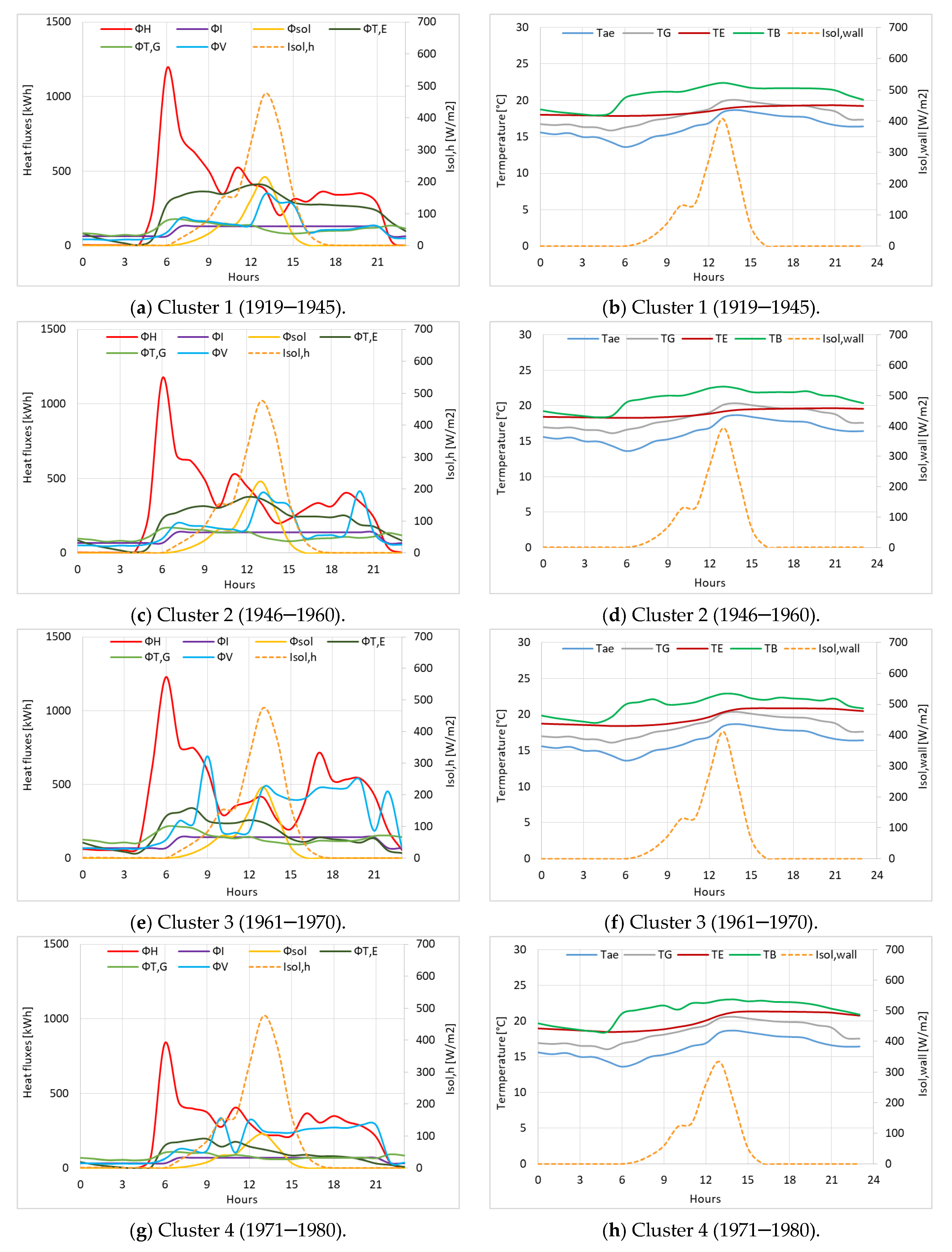
Figure 6, Figure 7, Figure 8 and Figure 9 show the trend of all the heat fluxes components and consequently the resulting trends of the temperatures of the three thermodynamic systems: building, opaque envelope, and glazing. The heat flux components in Equation (5) can be observed on the left; the heat flux through ventilation, ϕV (light blue), is quite constant. The temperatures of the three thermodynamic systems (B, E, and G) are represented, with the outside air temperature and the solar irradiance, on the right. These representations allowed us to control the input data and the weight of the energy balance components.
Figure 6 shows the results of the energy balance model with a number of constant air changes per hour of 0.5 h−1 over 24 hours for the typical day of February 22nd 2014, with a Tae= 6.24 °C. It can be observed that the temperature of the building, TB, (in green), has a constant diurnal and nighttime trend; the set-point range (20 ± 2 °C) is reached during the day. Similar results have been obtained applying the energy balance model with variable ventilation between daytime (ach = 0.62 h−1) and nighttime (0.3 h−1) in Figure 7. Compared to the previous model (with constant ventilation), during the day the dispersions due to ventilation are slightly higher, and consequently the temperature B is lower. Figure 8 and Figure 9 show results considering a variable number of air changes per hour and the opening of windows for typical days in February and October (the windows have been opened when the building temperature exceeds 22 °C). In Figure 8, the heat fluxes for February 22nd 2014 can be observed on the left with a clear difference in the heat flux from ventilation between the day and night and the high variation due to window openings. The temperature trend on the right is similar, but the temperature of the buildings does not exceed 22 °C.
The results of the energy balance model with a variable number of air changes per hour and the opening of windows have been presented also for a typical day in October, that is, October 24th 2013, with Tae = 16.3 °C (Figure 9). In general, it is possible to see, on the left, the increase in the ϕV, due to the windows opening at 2 p.m. A similar trend can be seen for clusters 3 and 4, where the windows were opened more times, with a consequent stabilization of the building temperature.
Figure 10 shows a representation of the positive and negative heat flux contributions for seven typical days that have been selected from Table 6 (remember that cluster 4 has a smaller useful surface area and volume). It is possible to observe that the heat flux for space heating is higher in the cold months of December and January, the thermal losses by transmission through opaque envelope and glazing and by ventilation vary according to the external local climate conditions and are higher in cold months, the internal gains are constant, and the solar gains through windows are higher in the warmer months (October, March and April).
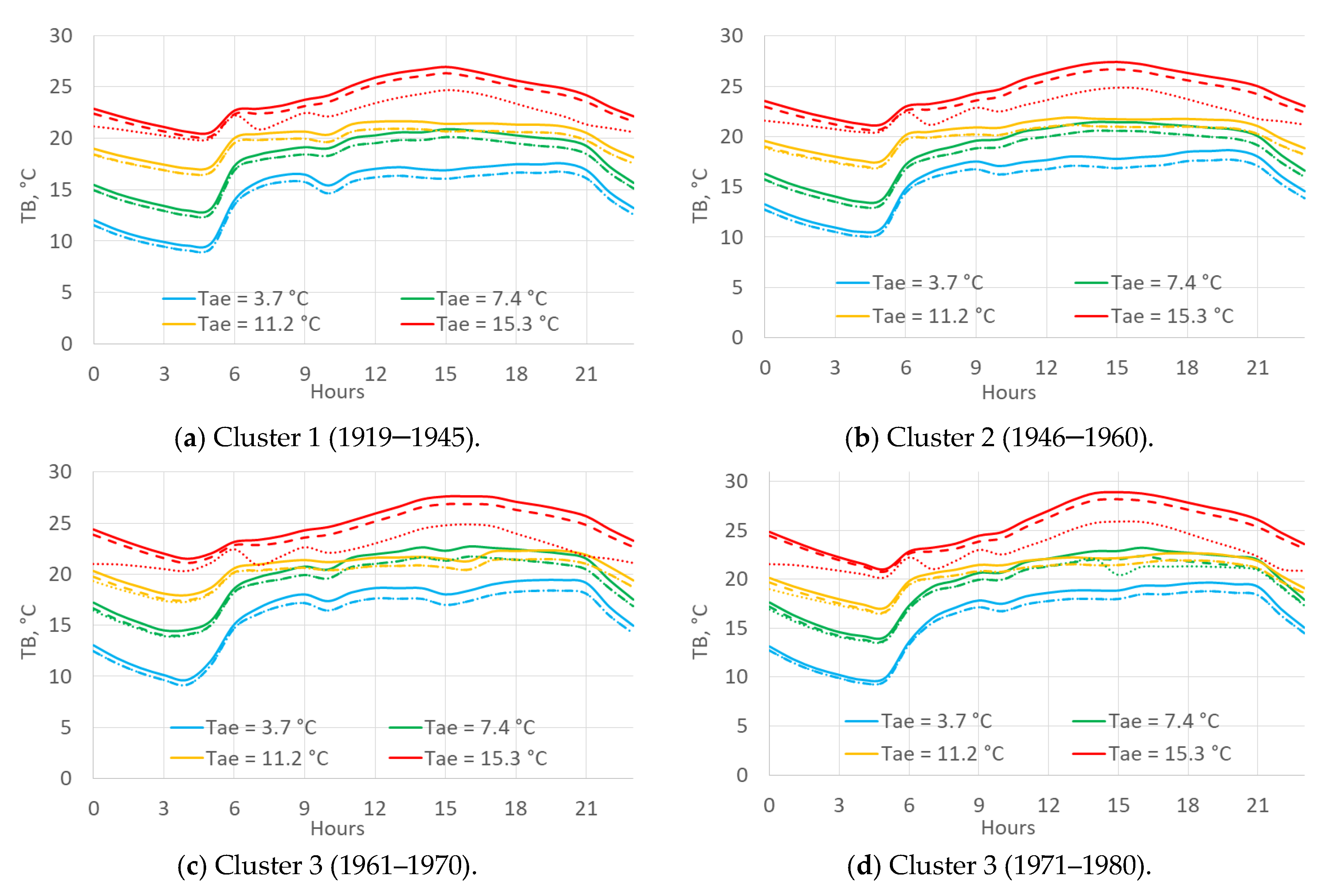
The building temperatures, TB, are represented in Figure 11, where the climate conditions for four typical days are shown, with a Tae = 3.7, 7.4, 11.2, and 15.3 °C. The solid lines represent the results of TB with constant ventilation with ach = 0.5 h−1, the dashed lines refer variable ventilation between daytime (ach = 0.62 h−1) and nighttime (0.3 h−1), and the dotted lines represent the ach variable and windows opening. The temperature of the three ventilation models is very similar for colder days. The difference with window openings can be observed only for higher temperatures (dotted lines).
Comparing the four clusters of buildings with different periods of construction, is possible to observe that the night and daytime building temperatures are quite stable and depend on both the characteristics of the buildings and on the external climatic conditions. This behavior suggests that it would be possible to hypothesize some correlations between the climatic conditions and the day and night temperatures of the building, TB.
The linear correlations between TB, Tair, and Tsol-air are reported in Figure 12 for the different ventilation conditions. In particular, Figure 12a,b presents the correlations with a constant ach = 0.5 h−1, Figure 12c,d considers a variable ach, and Figure 12e,f considers a variable ach with window opening. The main results are the following:
- Good correlations with TB are obtained for Tsol-air throughout the day (24 h) and daytime, while Tae was used for the nighttime (when solar irradiance cannot influence TB).
- Linear correlations are obtained with a good R2 coefficient of determination.
- Different correlations are obtained for the different clusters of buildings built in the four construction periods; the correlations with older buildings have a higher R2 and the values deviate less from the line of correlation with lower external temperatures.
- Different correlations are obtained for the different ventilation typologies; with variable ach and window openings, the lines of the correlation change the slope.
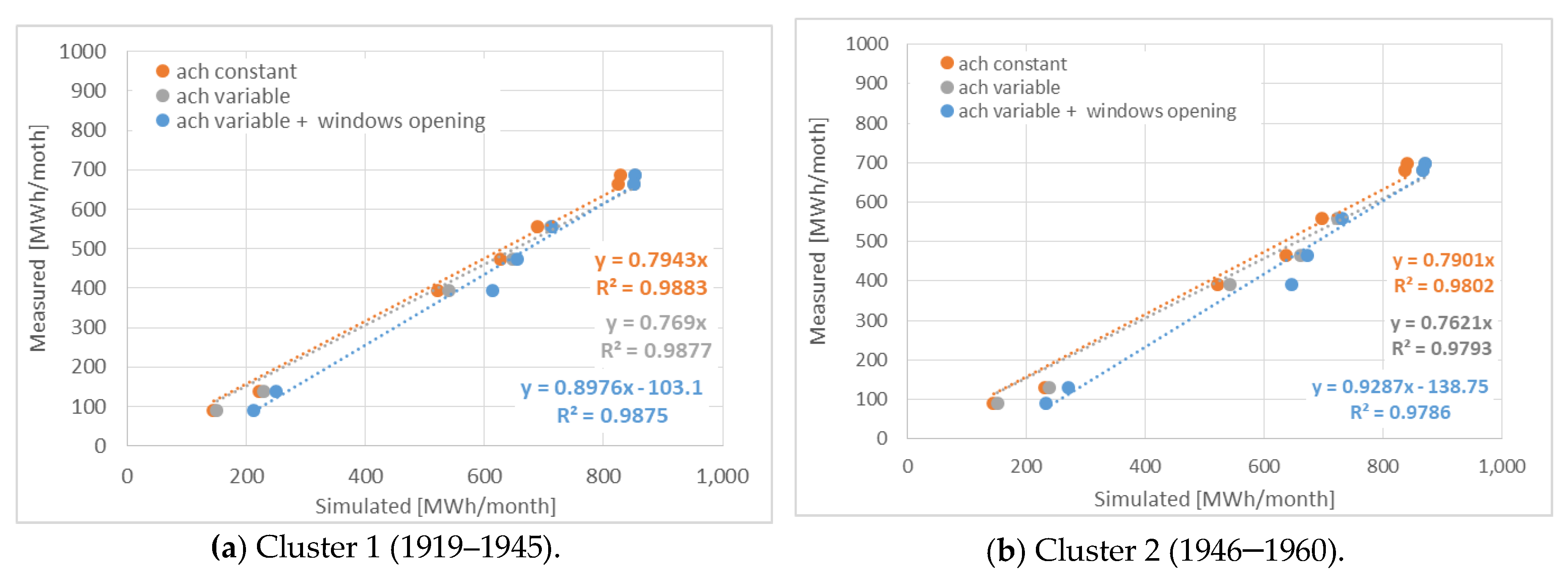
The Figure 13 shows the comparison between the simulated and measured daily thermal consumptions applying the model with the correlations for the building temperature and the three different ventilation conditions. A very good accuracy can be observed by comparing the simulated and measured values for each period of construction for the model with ach constant; the accuracy decreases with a variable ach and the last model with a variable ach and window openings is not accurate enough. This result attests that, in Turin, ventilation can be represented with the model of constant infiltration (during the analyzed heating period).
In Figure A1 of Appendix A, the comparison between the calculated and measured monthly energy consumption data are represented. The main conclusions are the same: the model that best represents the results is the one with constant ventilation; this model with a constant air change rate ach of 0.5 h−1 was chosen.
This type of model can be applied at the urban scale to represent the distribution of energy consumptions, evaluate the heat peak in every zone of a city, access the potential of renewable energy technologies that can be useful to meet that energy demand profile, and analyze the further expansion of a district heating network. All these applications can improve the security, sustainability, and affordability of the energy system and therefore the energy resilience of an urban environment.
In Figure 14, an example of the hourly model application to the city of Turin is represented. By changing the building attributes on the right, the results of this solution can be obtained.
5. Conclusions
In this work, the energy balance that has been studied for a single residential building has been simplified in order to use it at an urban scale with the existing databases (e.g., the Municipal Technical Maps that are available for every city), for groups of buildings with similar characteristics, and evaluate the distribution of space heating consumption in an urban context. The geometrical and typological characteristics of buildings were evaluated by geo-referencing information on building consumption using a GIS tool. This analysis was carried out on 92 residential buildings and on 4 groups of buildings with similar space heating consumptions and characteristics.
The main findings of the presented work can be summarized as follows:
- The presented model allows us to make fairly accurate forecasts on the consumption of buildings with the data available on an urban scale; of course, the existing tools are more accurate but do not allow analysis on cities, have much longer calculation times, and need data that is often not available.
- The best results were obtained with the building temperature variable according to the external climatic conditions and considering a constant ventilation by infiltrations of 0.5 ach.
- The use of a GIS tool allows us to design a very flexible urban-scale model, use data with different scales, manage the existing free databases, and map the results with a spatial distribution on the territory.
- Energy models and tools, such as the one proposed here, could be used at the territorial scale to:
- identify effective energy policies for the city, considering the real characteristics of buildings, population, and urban morphology;
- create an easily upgradable energy atlas for buildings, related to the existing territorial databases;
- evaluate the feasibility of establishing energy communities and grouping private and public entities, considering their energy consumptions and productions to reach energy security with a low environmental impact and good socio-economic effects.
The novelty of this simplified energy balance model concerns the possibility of applying it at the urban scale with the introduction of urban variables into the energy balance equations in order to consider the real characteristics of the urban context (with the sky view factor SVF, the urban canyon effect H/W ratio, and the solar exposition). These simplified engineering models can be used in an urban energy atlas to support decision-making in order to study how to improve the energy resilience of neighborhoods and cities with a place-based tool.
Author Contributions
Conceptualization, G.M.; Data curation, V.T.; Methodology, G.M. and V.T.; Software, V.T. and S.B.; Validation, G.M.; Writing—original draft, V.T.; Writing—review and editing, G.M. All authors have read and agreed to the published version of the manuscript.
Funding
This research received no external funding.
Conflicts of Interest
The authors declare no conflict of interest.
Nomenclature
| A | area, m2 | I | solar irradiance, Wm−2 |
| BCR | building coverage ratio, m2/m2 | ID | identity code, - |
| BD | building density, m3/m2 | MOS | main orientation of streets, - |
| c | specific heat capacity, Jkg−1K−1 | R | thermal resistance, m2KW−1 |
| C | effective heat capacity of a conditioned space (thermal capacity), JK−1 | S | net floor surface, m2 |
| DBT | territorial database, - | S/V | surface to volume ratio, m2/m3 |
| DH | district heating, - | SVF | sky view factor, - |
| DSM | digital surface model, - | t | time, s |
| F | reduction factor, - | T | temperature, °C |
| GHG | greenhouse gas, - | ||
| GIS | geographic information system, - | TS | thermodynamic system |
| h | surface coefficient of heat transfer, Wm−2K−1 | U | thermal transmittance, Wm−2K−1 |
| HDD | heating degree days, °C | V | volume, m3 |
| H/W | urban canyon height to width ratio, - | ||
| Greek symbols | |||
| α | absorption coefficient of solar radiation, - | λ | conductivity, Wm−1K−1 |
| ε | emissivity of a surface for long-wave thermal radiation, - | ξ | shadows percentage, - |
| η | system efficiency for space heating, - | τ | solar factor, - |
| ρ | density, kg/m3 | Φ | heat flow rate, thermal power, W |
| Subscripts | |||
| ae | external air | int | internal |
| B | building | k | building element |
| b | correction factor for unconditioned adjacent spaces | se | external surface |
| E | envelope | sol | solar |
| e | external | T | transmission |
| G | glazing | v | ventilation |
| H | heating | w | wall |
Appendix A

Table A1.
Characteristics of the analyzed 92 residential buildings connected to the DH network with the shutdown of the heating system at nighttime.
Table A1.
Characteristics of the analyzed 92 residential buildings connected to the DH network with the shutdown of the heating system at nighttime.
| ID | Period | Height [m] | Gross Vol. [m3] | Occup. [-] | S/V [m−1] | AW [m2] | AG [m2] | AE [m2] | H/W [-] | SVF [-] |
|---|---|---|---|---|---|---|---|---|---|---|
| 213 | 1919–1945 | 22.54 | 4983 | 0.93 | 0.28 | 803 | 166 | 1245 | 0.57 | 0.66 |
| 143 | 1919–1945 | 21.31 | 3905 | 0.63 | 0.29 | 646 | 115 | 1013 | 0.58 | 0.75 |
| 157 | 1919–1945 | 18.35 | 4804 | 0.88 | 0.33 | 896 | 164 | 1420 | 0.50 | 0.74 |
| 87 | 1919–1945 | 25.00 | 14,113 | 0.88 | 0.27 | 2286 | 423 | 3415 | 0.50 | 0.74 |
| 23 | 1919–1945 | 19.14 | 5078 | 0.91 | 0.27 | 684 | 166 | 1215 | 0.49 | 0.63 |
| 28 | 1919–1945 | 28.36 | 6593 | 0.77 | 0.29 | 1234 | 203 | 1699 | 0.55 | 0.62 |
| 36 | 1919–1945 | 14.98 | 5514 | 1.00 | 0.36 | 1069 | 184 | 1805 | 0.54 | 0.64 |
| 38 | 1919–1945 | 17.64 | 3236 | 0.91 | 0.30 | 497 | 92 | 864 | 0.49 | 0.63 |
| 48 | 1919–1945 | 15.10 | 5871 | 1.00 | 0.35 | 1090 | 194 | 1868 | 0.54 | 0.64 |
| 50 | 1919–1945 | 15.92 | 5405 | 0.91 | 0.29 | 702 | 170 | 1381 | 0.49 | 0.63 |
| 51 | 1919–1945 | 24.25 | 7225 | 1.00 | 0.26 | 1069 | 223 | 1665 | 0.54 | 0.64 |
| 55 | 1919–1945 | 19.72 | 11,175 | 0.87 | 0.28 | 1625 | 354 | 2759 | 0.55 | 0.63 |
| 212 | 1919–1945 | 19.78 | 4311 | 0.93 | 0.28 | 626 | 136 | 1062 | 0.57 | 0.66 |
| 94 | 1919–1945 | 19.01 | 3660 | 0.91 | 0.29 | 568 | 120 | 953 | 0.49 | 0.63 |
| 96 | 1919–1945 | 24.25 | 8476 | 1.00 | 0.29 | 1476 | 262 | 2175 | 0.54 | 0.64 |
| 99 | 1919–1945 | 24.25 | 8139 | 1.00 | 0.30 | 1496 | 252 | 2168 | 0.54 | 0.64 |
| 129 | 1919–1945 | 22.14 | 6986 | 0.81 | 0.26 | 943 | 237 | 1574 | 0.59 | 0.63 |
| 166 | 1919–1945 | 18.94 | 4960 | 0.87 | 0.32 | 917 | 164 | 1441 | 0.55 | 0.63 |
| 179 | 1919–1945 | 14.71 | 5484 | 1.00 | 0.36 | 1050 | 186 | 1796 | 0.54 | 0.64 |
| 17 | 1919–1945 | 20.55 | 6442 | 0.76 | 0.25 | 798 | 196 | 1425 | 0.57 | 0.62 |
| 61 | 1919–1945 | 21.88 | 9228 | 0.99 | 0.28 | 1386 | 316 | 2230 | 0.49 | 0.64 |
| 242 | 1919–1945 | 18.52 | 3773 | 0.93 | 0.27 | 495 | 127 | 902 | 0.50 | 0.62 |
| 218 | 1919–1945 | 23.92 | 12,156 | 1.00 | 0.26 | 1723 | 381 | 2739 | 0.54 | 0.64 |
| 122 | 1919–1945 | 23.68 | 4792 | 0.87 | 0.34 | 1050 | 152 | 1455 | 0.55 | 0.63 |
| 62 | 1919–1945 | 19.18 | 8897 | 0.91 | 0.29 | 1323 | 290 | 2251 | 0.49 | 0.63 |
| 103 | 1919–1945 | 22.00 | 12,825 | 0.92 | 0.24 | 1482 | 437 | 2648 | 0.58 | 0.71 |
| 52 | 1919–1945 | 25.10 | 16,387 | 0.95 | 0.21 | 1498 | 571 | 2804 | 0.56 | 0.75 |
| 132 | 1946–1960 | 21.89 | 8871 | 0.76 | 0.27 | 1269 | 304 | 2080 | 0.57 | 0.62 |
| 236 | 1946–1960 | 21.37 | 4039 | 0.82 | 0.26 | 547 | 118 | 925 | 0.52 | 0.65 |
| 92 | 1946–1960 | 29.95 | 7912 | 0.98 | 0.27 | 1372 | 264 | 1900 | 0.55 | 0.70 |
| 208 | 1946–1960 | 20.00 | 7428 | 0.82 | 0.29 | 1216 | 232 | 1959 | 0.52 | 0.65 |
| 5 | 1946–1960 | 22.77 | 4538 | 0.98 | 0.25 | 605 | 149 | 1004 | 0.55 | 0.70 |
| 6 | 1946–1960 | 22.89 | 4355 | 0.98 | 0.31 | 830 | 143 | 1210 | 0.55 | 0.70 |
| 14 | 1946–1960 | 19.55 | 3686 | 0.82 | 0.27 | 506 | 118 | 883 | 0.52 | 0.65 |
| 18 | 1946–1960 | 38.34 | 12,935 | 0.80 | 0.22 | 1720 | 422 | 2394 | 0.69 | 0.67 |
| 25 | 1946–1960 | 22.39 | 5460 | 0.88 | 0.32 | 1061 | 183 | 1549 | 0.50 | 0.74 |
| 35 | 1946–1960 | 27.56 | 7298 | 0.82 | 0.26 | 1108 | 232 | 1637 | 0.52 | 0.65 |
| 108 | 1946–1960 | 19.47 | 6291 | 0.76 | 0.29 | 999 | 202 | 1645 | 0.57 | 0.62 |
| 147 | 1946–1960 | 24.28 | 8740 | 0.76 | 0.26 | 1303 | 270 | 2023 | 0.57 | 0.62 |
| 222 | 1946–1960 | 21.11 | 6807 | 0.82 | 0.25 | 874 | 202 | 1519 | 0.52 | 0.65 |
| 238 | 1946–1960 | 19.47 | 4930 | 0.76 | 0.27 | 658 | 158 | 1164 | 0.57 | 0.62 |
| 146 | 1946–1960 | 22.31 | 8668 | 0.95 | 0.26 | 1223 | 291 | 2000 | 0.56 | 0.75 |
| 187 | 1946–1960 | 19.50 | 3600 | 0.82 | 0.27 | 470 | 115 | 839 | 0.52 | 0.65 |
| 67 | 1946–1960 | 27.64 | 5097 | 0.82 | 0.24 | 698 | 161 | 1067 | 0.52 | 0.65 |
| 64 | 1946–1960 | 19.69 | 8927 | 0.93 | 0.28 | 1333 | 283 | 2239 | 0.57 | 0.66 |
| 162 | 1946–1960 | 21.77 | 4296 | 0.87 | 0.30 | 745 | 148 | 1140 | 0.55 | 0.63 |
| 198 | 1946–1960 | 27.84 | 8535 | 0.80 | 0.26 | 1346 | 268 | 1959 | 0.69 | 0.67 |
| 181 | 1946–1960 | 24.98 | 3743 | 0.91 | 0.27 | 614 | 112 | 914 | 0.49 | 0.63 |
| 177 | 1946–1960 | 19.10 | 5151 | 0.93 | 0.29 | 773 | 169 | 1313 | 0.57 | 0.63 |
| 133 | 1946–1960 | 19.28 | 3689 | 0.87 | 0.33 | 724 | 120 | 1106 | 0.53 | 0.66 |
| 3 | 1946–1960 | 20.98 | 4389 | 0.93 | 0.29 | 736 | 131 | 1155 | 0.57 | 0.63 |
| 69 | 1946–1960 | 28.00 | 8008 | 0.82 | 0.25 | 1171 | 250 | 1743 | 0.52 | 0.65 |
| 193 | 1946–1960 | 15.49 | 10,486 | 0.76 | 0.35 | 2021 | 338 | 3374 | 0.53 | 0.63 |
| 111 | 1946–1960 | 24.24 | 9050 | 0.93 | 0.30 | 1656 | 280 | 2403 | 0.50 | 0.62 |
| 88 | 1946–1960 | 23.92 | 9954 | 1.00 | 0.30 | 1843 | 312 | 2675 | 0.54 | 0.64 |
| 171 | 1946–1960 | 24.53 | 9472 | 0.76 | 0.26 | 1398 | 290 | 2170 | 0.57 | 0.62 |
| 188 | 1946–1960 | 19.60 | 5094 | 0.82 | 0.26 | 631 | 162 | 1151 | 0.52 | 0.65 |
| 130 | 1946–1960 | 25.95 | 5008 | 0.76 | 0.27 | 814 | 169 | 1200 | 0.57 | 0.62 |
| 221 | 1946–1960 | 28.41 | 5892 | 0.80 | 0.25 | 876 | 181 | 1291 | 0.69 | 0.67 |
| 74 | 1961–1970 | 24.82 | 11,337 | 0.80 | 0.28 | 1960 | 343 | 2874 | 0.37 | 0.78 |
| 240 | 1961–1970 | 23.04 | 3349 | 0.98 | 0.24 | 390 | 109 | 680 | 0.55 | 0.70 |
| 45 | 1961–1970 | 13.00 | 8324 | 0.87 | 0.32 | 1162 | 240 | 2443 | 0.55 | 0.63 |
| 9 | 1961–1970 | 28.10 | 6528 | 0.98 | 0.24 | 880 | 203 | 1345 | 0.55 | 0.70 |
| 22 | 1961–1970 | 23.95 | 5968 | 0.93 | 0.26 | 837 | 187 | 1336 | 0.57 | 0.66 |
| 72 | 1961–1970 | 29.85 | 8121 | 0.80 | 0.27 | 1378 | 272 | 1922 | 0.37 | 0.78 |
| 76 | 1961–1970 | 30.57 | 5743 | 0.95 | 0.28 | 1018 | 188 | 1394 | 0.56 | 0.75 |
| 173 | 1961–1970 | 18.68 | 7234 | 0.93 | 0.27 | 901 | 242 | 1675 | 0.50 | 0.62 |
| 185 | 1961–1970 | 24.03 | 4616 | 0.93 | 0.29 | 825 | 144 | 1210 | 0.57 | 0.66 |
| 202 | 1961–1970 | 22.55 | 12,232 | 0.76 | 0.26 | 1741 | 407 | 2826 | 0.57 | 0.62 |
| 210 | 1961–1970 | 28.10 | 6342 | 0.98 | 0.30 | 1253 | 197 | 1705 | 0.55 | 0.70 |
| 227 | 1961–1970 | 20.19 | 1800 | 0.81 | 0.38 | 454 | 56 | 633 | 0.59 | 0.63 |
| 12 | 1961–1970 | 23.39 | 5422 | 0.87 | 0.23 | 617 | 174 | 1081 | 0.53 | 0.66 |
| 83 | 1961–1970 | 18.92 | 3869 | 0.93 | 0.28 | 527 | 128 | 936 | 0.57 | 0.63 |
| 32 | 1961–1970 | 23.56 | 4340 | 0.90 | 0.29 | 738 | 138 | 1106 | 0.52 | 0.66 |
| 159 | 1961–1970 | 22.09 | 8191 | 0.87 | 0.31 | 1520 | 278 | 2262 | 0.53 | 0.66 |
| 58 | 1961–1970 | 15.50 | 4179 | 0.99 | 0.41 | 1057 | 135 | 1596 | 0.49 | 0.64 |
| 7 | 1961–1970 | 28.10 | 6916 | 0.98 | 0.24 | 970 | 215 | 1463 | 0.55 | 0.70 |
| 97 | 1961–1970 | 26.49 | 28,450 | 0.93 | 0.23 | 3528 | 940 | 5676 | 0.50 | 0.62 |
| 201 | 1961–1970 | 24.00 | 25,968 | 0.95 | 0.27 | 3995 | 811 | 6159 | 0.56 | 0.75 |
| 77 | 1961–1970 | 28.00 | 28,398 | 0.95 | 0.25 | 4067 | 1014 | 6095 | 0.56 | 0.75 |
| 246 | 1961–1970 | 21.29 | 2793 | 0.77 | 0.30 | 490 | 82 | 753 | 0.55 | 0.62 |
| 20 | 1971–1980 | 26.23 | 20,994 | 1.00 | 0.33 | 3738 | 700 | 5339 | 0.57 | 0.69 |
| 21 | 1971–1980 | 29.78 | 5273 | 0.89 | 0.41 | 1338 | 177 | 1692 | 0.78 | 0.68 |
| 24 | 1971–1980 | 36.58 | 10,876 | 0.89 | 0.30 | 1847 | 372 | 2442 | 0.78 | 0.68 |
| 56 | 1971–1980 | 29.70 | 4524 | 0.89 | 0.40 | 1117 | 152 | 1421 | 0.78 | 0.68 |
| 58 | 1971–1980 | 36.51 | 6846 | 0.89 | 0.42 | 1911 | 234 | 2286 | 0.78 | 0.68 |
| 59 | 1971–1980 | 29.28 | 7514 | 0.89 | 0.39 | 1779 | 257 | 2292 | 0.78 | 0.68 |
| 95 | 1971–1980 | 36.72 | 10,537 | 0.89 | 0.37 | 2454 | 359 | 3028 | 0.78 | 0.68 |
| 119 | 1971–1980 | 25.00 | 17,362 | 0.92 | 0.27 | 2793 | 521 | 4182 | 0.58 | 0.71 |
| 65 | 1971–1980 | 29.00 | 12,364 | 0.93 | 0.32 | 2707 | 426 | 3560 | 0.57 | 0.66 |
| 190 | 1971–1980 | 20.36 | 4912 | 0.91 | 0.36 | 917 | 151 | 1399 | 0.53 | 0.64 |
| 100 | 1971–1980 | 17.96 | 13,494 | 0.96 | 0.34 | 2080 | 470 | 3583 | 0.28 | 0.73 |
Figure A1 shows the comparison between the simulated and measured monthly thermal consumptions. The simulated thermal consumptions have been calculated using the three dynamic thermal balances: (i) a constant air change rate n = 0.5 h−1; (ii) a variable ach during the daytime and nighttime; (iii) a variable ach considering a quota for infiltrations and a quota for window openings.
Figure A1.
Comparison between the simulated and measured monthly thermal consumptions, distinguishing ach = 0.5 h−1 (in orange), ach = 0.62 h−1 during the daytime, ach = 0.3 h−1 during the nighttime (in grey), and variable ach with window openings (in blue).
Figure A1.
Comparison between the simulated and measured monthly thermal consumptions, distinguishing ach = 0.5 h−1 (in orange), ach = 0.62 h−1 during the daytime, ach = 0.3 h−1 during the nighttime (in grey), and variable ach with window openings (in blue).


References
- Rosenow, J.; Cowart, R.; Bayer, E.; Fabbri, M. Assessing the European Union’s energy efficiency policy: Will the winter package deliver on ‘Efficiency First’? Energy Res. Soc. Sci. 2017, 26, 72–79. [Google Scholar] [CrossRef]
- Brunetta, G.; Ceravolo, R.; Barbieri, C.A.; Borghini, A.; De Carlo, F.; Mela, A.; Beltramo, S.; Longhi, A.; De Lucia, G.; Ferraris, S.; et al. Territorial Resilience: Toward a Proactive Meaning for Spatial Planning. Sustainability 2019, 11, 2286. [Google Scholar] [CrossRef] [Green Version]
- Brunetta, G.; Salata, S. Mapping Urban Resilience for Spatial Planning—A First Attempt to Measure the Vulnerability of the System. Sustainability 2019, 11, 2331. [Google Scholar] [CrossRef] [Green Version]
- Doost, D.M.; Buffa, A.; Brunetta, G.; Salata, S.; Mutani, G. Mainstreaming Energetic Resilience by Morphological Assessment in Ordinary Land Use Planning. The Case Study of Moncalieri, Turin (Italy). Sustainability 2020, 12, 4443. [Google Scholar] [CrossRef]
- Hedegaard, R.E.; Kristensen, M.H.; Pedersen, T.H.; Brun, A.; Petersen, S. Bottom-up modelling methodology for urban-scale analysis of residential space heating demand response. Appl. Energy 2019, 242, 181–204. [Google Scholar] [CrossRef]
- Boghetti, R.; Fantozzi, F.; Kämpf, J.H.; Mutani, G.; Salvadori, G.; Todeschi, V. Building energy models with Morphological urban-scale parameters: A case study in Turin. In Proceedings of the 4th Building Simulation Applications Conference—BSA, Bozen-Bolzano, Italy, 19–21 June 2019; pp. 1–8. [Google Scholar]
- Gobakis, K.; Kolokotsa, D. Coupling building energy simulation software with microclimatic simulation for the evaluation of the impact of urban outdoor conditions on the energy consumption and indoor environmental quality. Energy Build. 2017, 157, 101–115. [Google Scholar] [CrossRef]
- Sola, A.; Corchero, C.; Salom, J.; Sanmarti, M. Simulation Tools to Build Urban-Scale Energy Models: A Review. Energies 2018, 11, 3269. [Google Scholar] [CrossRef] [Green Version]
- Sola, A.; Corchero, C.; Salom, J.; Sanmarti, M. Multi-domain urban-scale energy modelling tools: A review. Sustain. Cities Soc. 2020, 54, 101872. [Google Scholar] [CrossRef]
- Abbasabadi, N.; Ashayeri, M. Urban energy use modeling methods and tools: A review and an outlook. Build. Environ. 2019, 161, 106270. [Google Scholar] [CrossRef]
- Yang, F.; Jiang, Z. Urban building energy modelling and urban design for sustainable neighborhood development-A China perspective. IOP Conf. Ser. Earth Environ. Sci. 2019, 329, 012016. [Google Scholar] [CrossRef]
- Ward, H.C.; Kotthaus, S.; Järvi, L.; Grimmond, C.S.B. Surface Urban Energy and Water Balance Scheme (SUEWS): Development and evaluation at two UK sites. Urban Clim. 2016, 18, 1–32. [Google Scholar] [CrossRef] [Green Version]
- Vallati, A.; Grignaffini, S.; Romagna, M.; Mauri, L.; Colucci, C. Influence of Street Canyon’s Microclimate on the Energy Demand for Space Cooling and Heating of Buildings. Energy Procedia 2016, 101, 941–947. [Google Scholar] [CrossRef]
- Huang, J.; Jones, P.; Zhang, A.; Peng, R.; Li, X.; Chan, P.-W. Urban Building Energy and Climate (UrBEC) simulation: Example application and field evaluation in Sai Ying Pun, Hong Kong. Energy Build. 2020, 207, 109580. [Google Scholar] [CrossRef]
- Lauzet, N.; Rodler, A.; Musy, M.; Azam, M.-H.; Guernouti, S.; Mauree, D.; Colinart, T. How building energy models take the local climate into account in an urban context—A review. Renew. Sustain. Energy Rev. 2019, 116, 109390. [Google Scholar] [CrossRef]
- Sharifi, A.; Yamagata, Y. A Conceptual Framework for Assessment of Urban Energy Resilience. Energy Procedia 2015, 75, 2904–2909. [Google Scholar] [CrossRef] [Green Version]
- Sharifi, A.; Yamagata, Y. Principles and criteria for assessing urban energy resilience: A literature review. Renew. Sustain. Energy Rev. 2016, 60, 1654–1677. [Google Scholar] [CrossRef] [Green Version]
- Ohshita, S.; Johnson, K. Resilient urban energy: Making city systems energy efficient, low carbon, and resilient in a changing climate. ECEEE Summer Study Proc. 2017, 719–728. [Google Scholar]
- Sugahara, M.; Bermont, L. Energy and Resilient Cities. OECD Reg. Dev. Work. Papers 2016. [Google Scholar] [CrossRef]
- Chen, Y.; Hong, T.; Piette, M.A. Automatic generation and simulation of urban building energy models based on city datasets for city-scale building retrofit analysis. Appl. Energy 2017, 205, 323–335. [Google Scholar] [CrossRef] [Green Version]
- Luo, X.; Hong, T.; Tang, Y.-H. Modeling Thermal Interactions between Buildings in an Urban Context. Energies 2020, 13, 2382. [Google Scholar] [CrossRef]
- Walter, E.; Kämpf, J.H.; Baratieri, M.; Corrado, V.; Gasparella, A.; Patuzzi, F. A Verification of CitySim Results Using the BESTEST and Monitored Consumption Values. Available online: https://infoscience.epfl.ch/record/214754 (accessed on 14 July 2020).
- Zhu, P.; Yan, D.; Sun, H.; An, J.; Huang, Y. Building Blocks Energy Estimation (BBEE): A method for building energy estimation on district level. Energy Build. 2019, 185, 137–147. [Google Scholar] [CrossRef]
- Olivo, Y.; Hamidi, A.; Ramamurthy, P. Spatiotemporal variability in building energy use in New York City. Energy 2017, 141, 1393–1401. [Google Scholar] [CrossRef]
- Ahmed, K.; Ortiz, L.E.; Gonzalez, J. On the Spatio-Temporal End-User Energy Demands of a Dense Urban Environment. J. Sol. Energy Eng. 2017, 139, 041005. [Google Scholar] [CrossRef]
- Takane, Y.; Kikegawa, Y.; Hara, M.; Ihara, T.; Ohashi, Y.; Adachi, S.; Kondo, H.; Yamaguchi, K.; Kaneyasu, N. A climatological validation of urban air temperature and electricity demand simulated by a regional climate model coupled with an urban canopy model and a building energy model in an Asian megacity. Int. J. Clim. 2017, 37, 1035–1052. [Google Scholar] [CrossRef]
- Salamanca, F.; Krpo, A.; Martilli, A.; Clappier, A. A new building energy model coupled with an urban canopy parameterization for urban climate simulations—part I. formulation, verification, and sensitivity analysis of the model. Theor. Appl. Clim. 2009, 99, 331–344. [Google Scholar] [CrossRef]
- Jain, R.; Smith, K.; Culligan, P.J.; Taylor, J.E. Forecasting energy consumption of multi-family residential buildings using support vector regression: Investigating the impact of temporal and spatial monitoring granularity on performance accuracy. Appl. Energy 2014, 123, 168–178. [Google Scholar] [CrossRef]
- Mutani, G.; Todeschi, V.; Kaempf, J.; Coors, V.; Fitzky, M. Building energy consumption modeling at urban scale: Three case studies in Europe for residential buildings. In Proceedings of the 2018 IEEE International Telecommunications Energy Conference (INTELEC), Turin, Italy, 7–11 October 2018; pp. 1–8. [Google Scholar]
- Mutani, G.; Todeschi, V. Space heating models at urban scale for buildings in the city of Turin (Italy). Energy Procedia 2017, 122, 841–846. [Google Scholar] [CrossRef] [Green Version]
- Mutani, G.; Todeschi, V. Energy Resilience, Vulnerability and Risk in Urban Spaces. J. Sustain. Dev. Energy Water Environ. Syst. 2018, 6, 694–709. [Google Scholar] [CrossRef] [Green Version]
- Wei, Y.; Zhang, X.; Shi, Y.; Xia, L.; Pan, S.; Wu, J.; Han, M.; Zhao, X. A review of data-driven approaches for prediction and classification of building energy consumption. Renew. Sustain. Energy Rev. 2018, 82, 1027–1047. [Google Scholar] [CrossRef]
- Mutani, G.; Todeschi, V.; Guelpa, E.; Verda, V. Building Efficiency Models and the Optimization of the District Heating Network for Low-Carbon Transition Cities. In Improving Energy Efficiency in Commercial Buildings and Smart Communities; Springer Proceeding in Energy; Springer: Cham, Switzerland, 2020; pp. 217–241. [Google Scholar]
- Kikegawa, Y.; Genchi, Y.; Yoshikado, H.; Kondo, H. Development of a numerical simulation system toward comprehensive assessments of urban warming countermeasures including their impacts upon the urban buildings’ energy-demands. Appl. Energy 2003, 76, 449–466. [Google Scholar] [CrossRef]
- Alhamwi, A.; Medjroubi, W.; Vogt, T.; Agert, C. GIS-based urban energy systems models and tools: Introducing a model for the optimisation of flexibilisation technologies in urban areas. Appl. Energy 2017, 191, 1–9. [Google Scholar] [CrossRef]
- AA.VV.—TABULA Typology Approach for Building Stock Energy Assessment—TABULA. 2012. Available online: http://webtool.building-typology.eu/#bm (accessed on 5 January 2020).
- Duffie, J.A.; Beckman, W.A. Solar Engineering of Thermal Processes, 4th ed.; Wiley: Hoboken, NJ, USA, 2013; ISBN 9780470873663. [Google Scholar]
- Miguel, A.F. Constructal design of solar energy-based systems for buildings. Energy Build. 2008, 40, 1020–1030. [Google Scholar] [CrossRef]
- Mutani, G.; Todeschi, V.; Matsuo, K. Urban Heat Island Mitigation: A GIS-based Model for Hiroshima. Instrum. Mes. Metrol. 2019, 18, 323–335. [Google Scholar] [CrossRef]
- Streicher, K.N.; Padey, P.; Parra, D.; Bürer, M.C.; Schneider, S.; Patel, M.K. Analysis of space heating demand in the Swiss residential building stock: Element-based bottom-up model of archetype buildings. Energy Build. 2019, 184, 300–322. [Google Scholar] [CrossRef]
- Xu, X.; AzariJafari, H.; Gregory, J.; Norford, L.; Kirchain, R. An integrated model for quantifying the impacts of pavement albedo and urban morphology on building energy demand. Energy Build. 2020, 211, 109759. [Google Scholar] [CrossRef]
- Mutani, G.; Todeschi, V. The Effects of Green Roofs on Outdoor Thermal Comfort, Urban Heat Island Mitigation and Energy Savings. Atmosphere (Basel) 2020, 11, 123. [Google Scholar] [CrossRef] [Green Version]
- Muniz-Gäal, L.P.; Pezzuto, C.C.; De Carvalho, M.F.H.; Mota, L.T.M. Urban geometry and the microclimate of street canyons in tropical climate. Build. Environ. 2020, 169, 106547. [Google Scholar] [CrossRef]
- Ahn, Y.; Sohn, D.-W. The effect of neighbourhood-level urban form on residential building energy use: A GIS-based model using building energy benchmarking data in Seattle. Energy Build. 2019, 196, 124–133. [Google Scholar] [CrossRef]
- Mutani, G.; Perino, M. Ventilazione naturale mediante apertura controllata di finestre: Implicazioni sul comfort interno. In Proceedings of the 41° AICARR Conference, Milano, Italy, 22–23 March 2000; pp. 1049–1065. [Google Scholar]
- Mutani, G.; Todeschi, V. An Urban Energy Atlas and Engineering Model for Resilient Cities. Int. J. Heat Technol. 2019, 37, 936–947. [Google Scholar] [CrossRef] [Green Version]
- Mutani, G.; Giaccardi, F.; Martino, M.; Pastorelli, M. Modeling hourly profile of space heating energy consumption for residential buildings. In Proceedings of the 2017 IEEE International Telecommunications Energy Conference (INTELEC), Broadbeach, QLD, Australia, 22–26 October 2017; pp. 245–253. [Google Scholar]
Figure 1.
Flowchart of the methodology.

Figure 2.
Shadow percentage assessment (an example for two days in April and December).
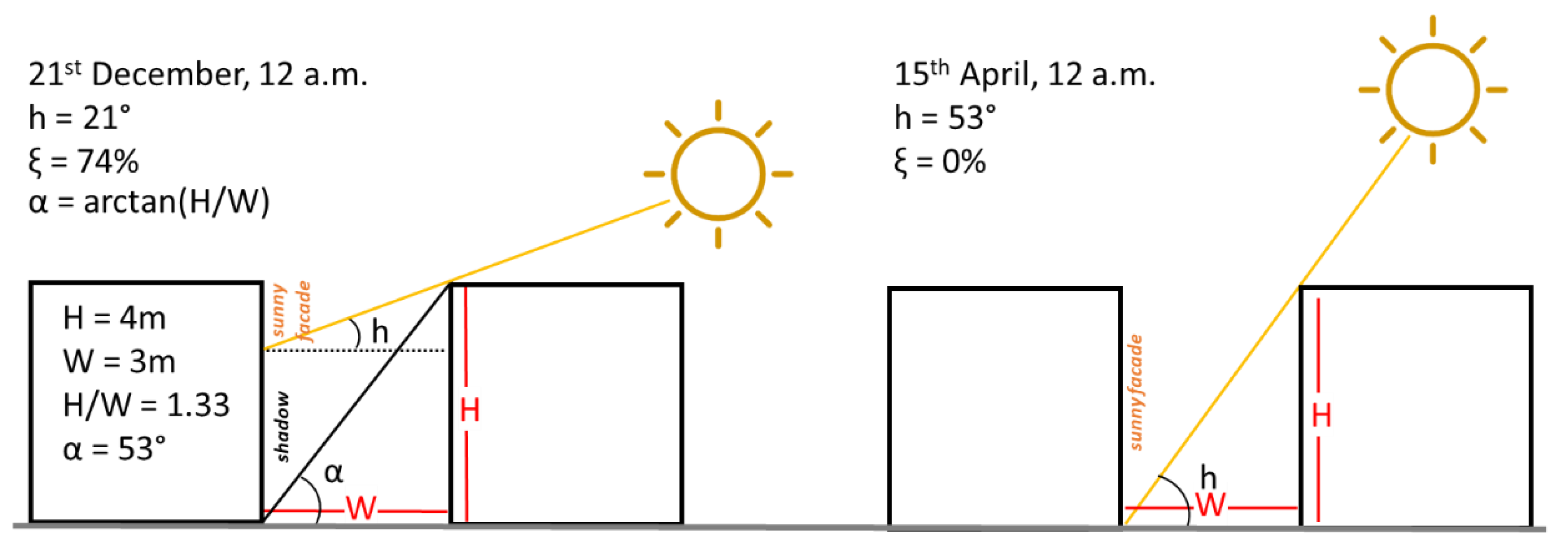
Figure 3.
The three thermodynamic systems of the dynamic engineering model: B = internal structures of the building, furniture, and air; E = opaque envelope; G = transparent envelope (glass).
Figure 3.
The three thermodynamic systems of the dynamic engineering model: B = internal structures of the building, furniture, and air; E = opaque envelope; G = transparent envelope (glass).
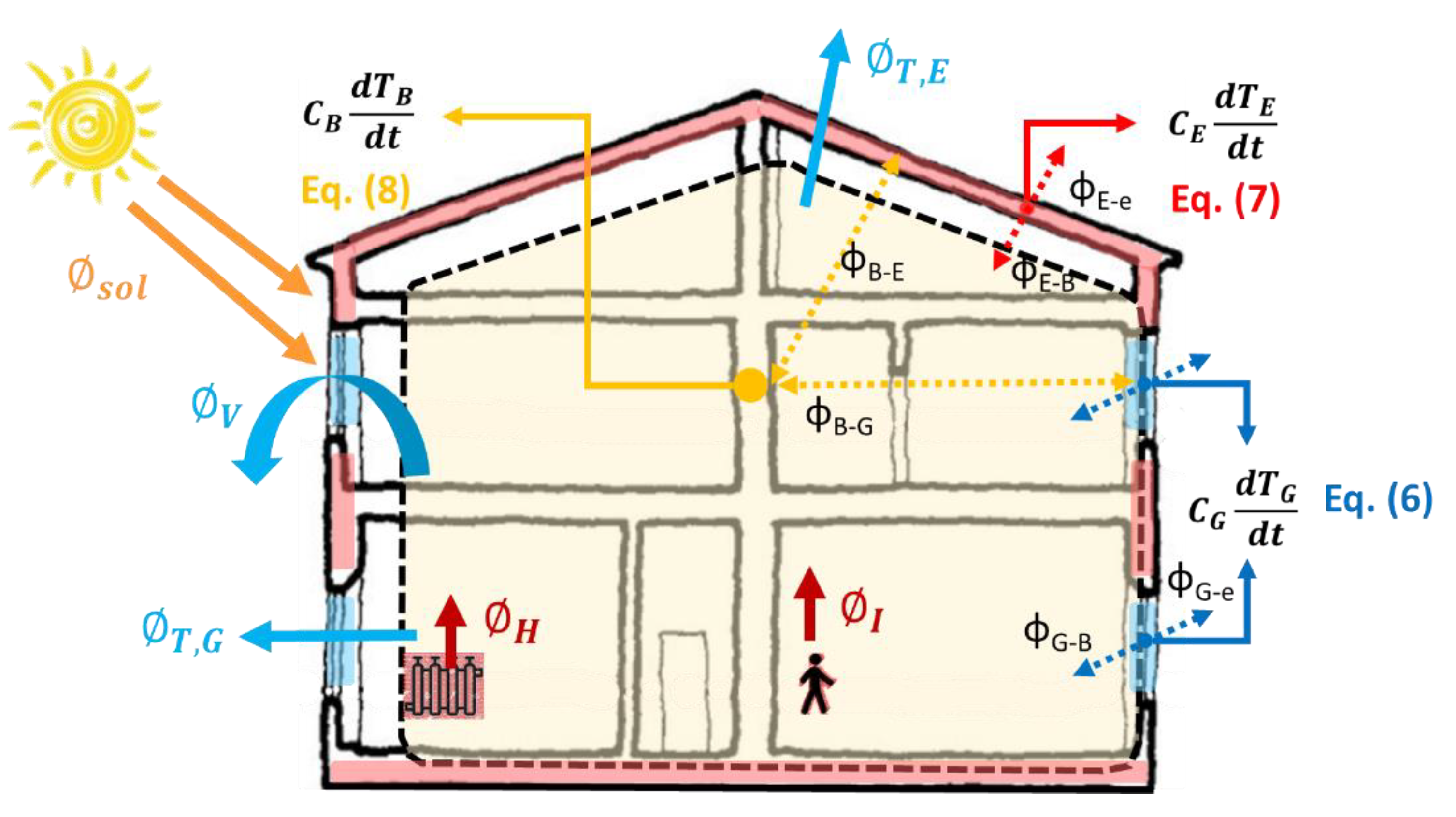
Figure 4.
Correlation between ΔT = (Tai – Tae) (°C) and the number of air exchanges per hour; measured data for typical Italian windows with a height = 1.5 m [45].
Figure 4.
Correlation between ΔT = (Tai – Tae) (°C) and the number of air exchanges per hour; measured data for typical Italian windows with a height = 1.5 m [45].

Figure 5.
Space heating hourly consumptions (Wh/m3) with different Tae—(a) 1.7 °C, (b) 4.3 °C, (c) 8.7 °C, (d) 12.5 °C—for four clusters of buildings: cluster 1—1919–1945; cluster 2—1946–1960; cluster 3—1961–1970; cluster 4—1971–1980.
Figure 5.
Space heating hourly consumptions (Wh/m3) with different Tae—(a) 1.7 °C, (b) 4.3 °C, (c) 8.7 °C, (d) 12.5 °C—for four clusters of buildings: cluster 1—1919–1945; cluster 2—1946–1960; cluster 3—1961–1970; cluster 4—1971–1980.
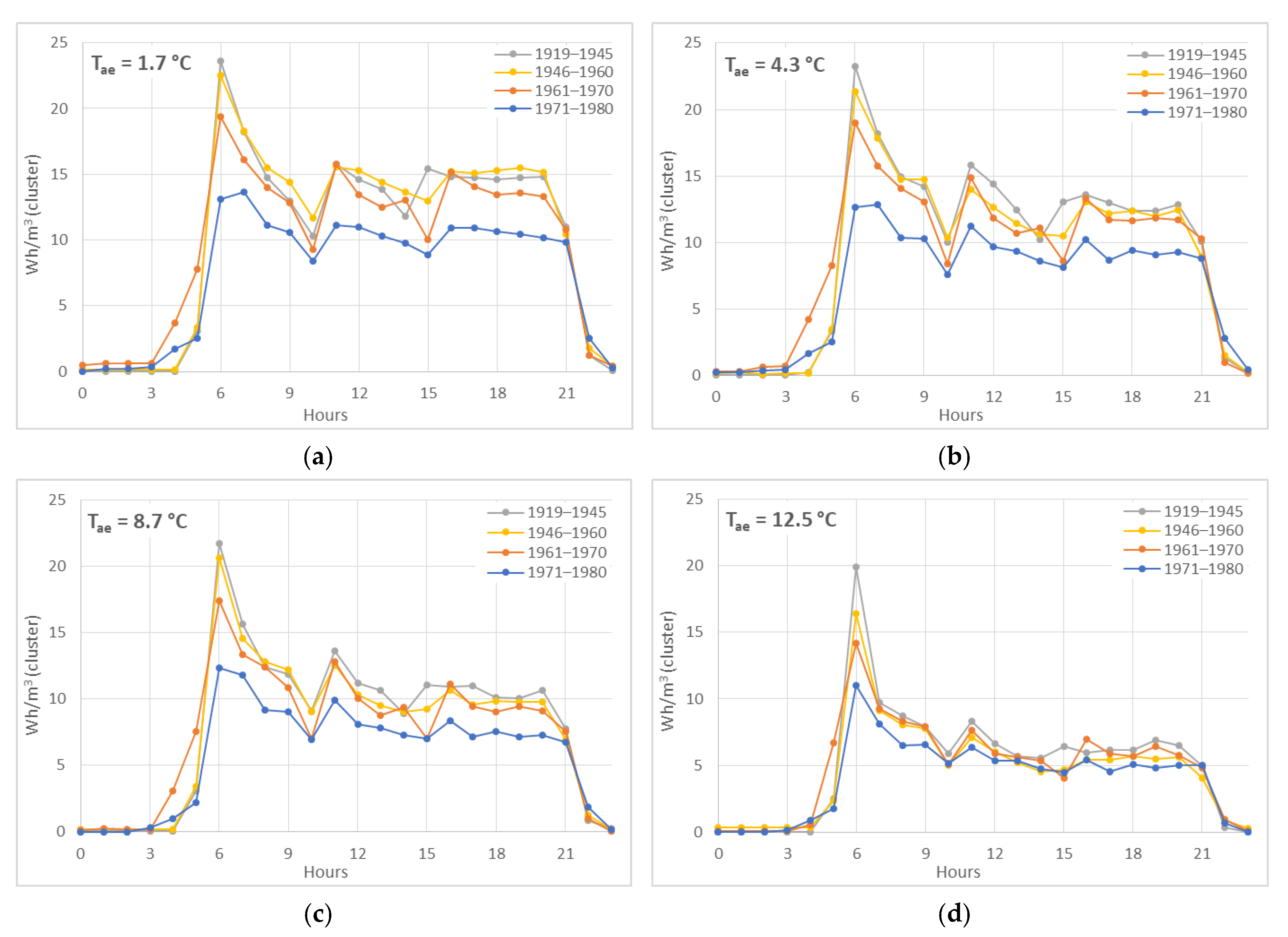
Figure 6.
Heat flux components and building temperatures (with constant ach = 0.5 h−1) for a typical day: February 22nd 2014, with a Tae= 6.24 °C (clusters for the four construction periods).
Figure 6.
Heat flux components and building temperatures (with constant ach = 0.5 h−1) for a typical day: February 22nd 2014, with a Tae= 6.24 °C (clusters for the four construction periods).

Figure 7.
Heat flux components and building temperatures with a variable number of air changes per hour (in daytime ach = 0.62 h−1, and in nighttime ach = 0.3 h−1) for a typical day: February 22nd 2014, with a Tae= 6.24 °C (clusters for the four construction periods).
Figure 7.
Heat flux components and building temperatures with a variable number of air changes per hour (in daytime ach = 0.62 h−1, and in nighttime ach = 0.3 h−1) for a typical day: February 22nd 2014, with a Tae= 6.24 °C (clusters for the four construction periods).
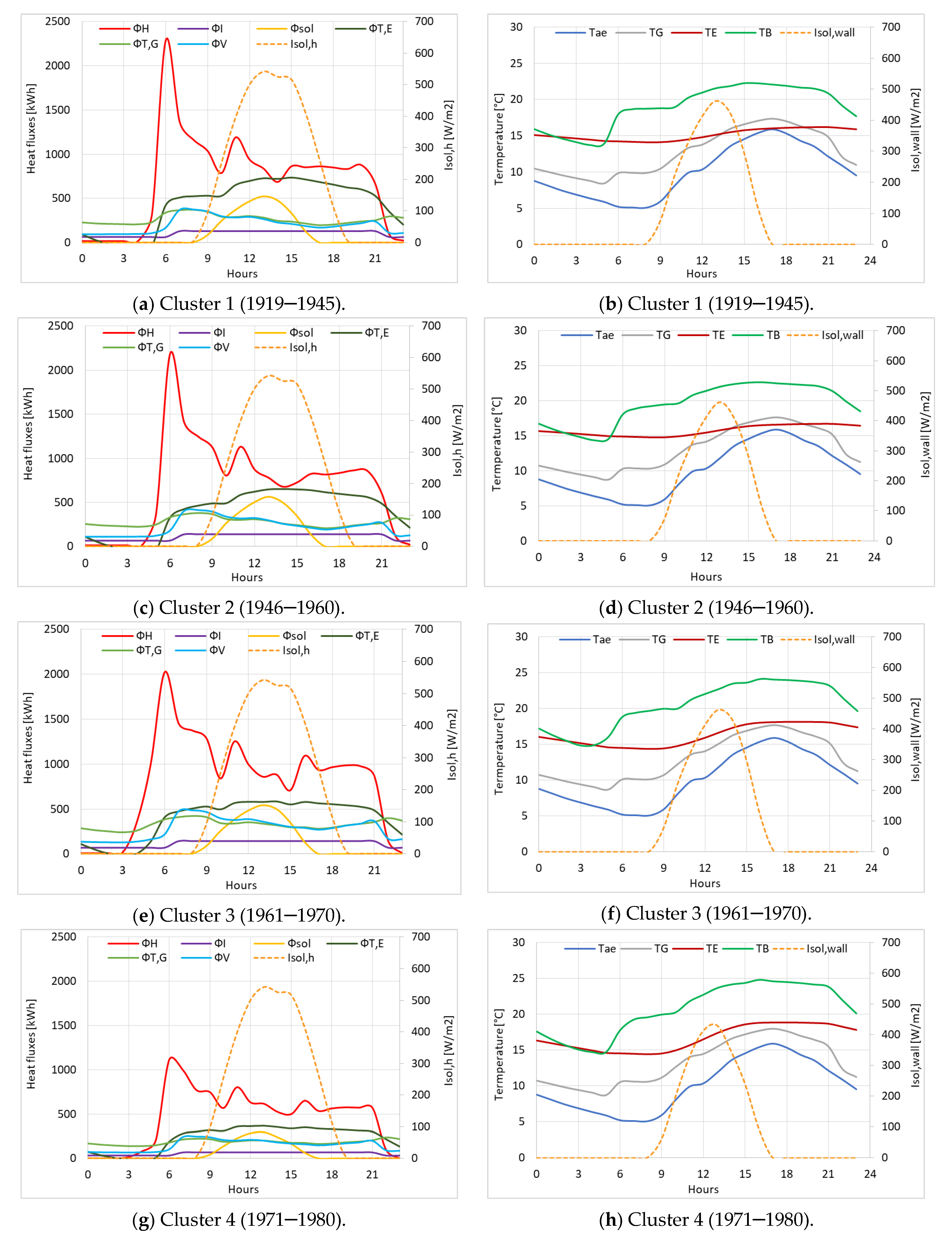
Figure 8.
Heat flux components and building temperatures (with a variable number of air changes per hour and windows opening) for a typical day: February 22nd 2014, with a Tae= 6.24 °C (clusters for the four construction periods).
Figure 8.
Heat flux components and building temperatures (with a variable number of air changes per hour and windows opening) for a typical day: February 22nd 2014, with a Tae= 6.24 °C (clusters for the four construction periods).
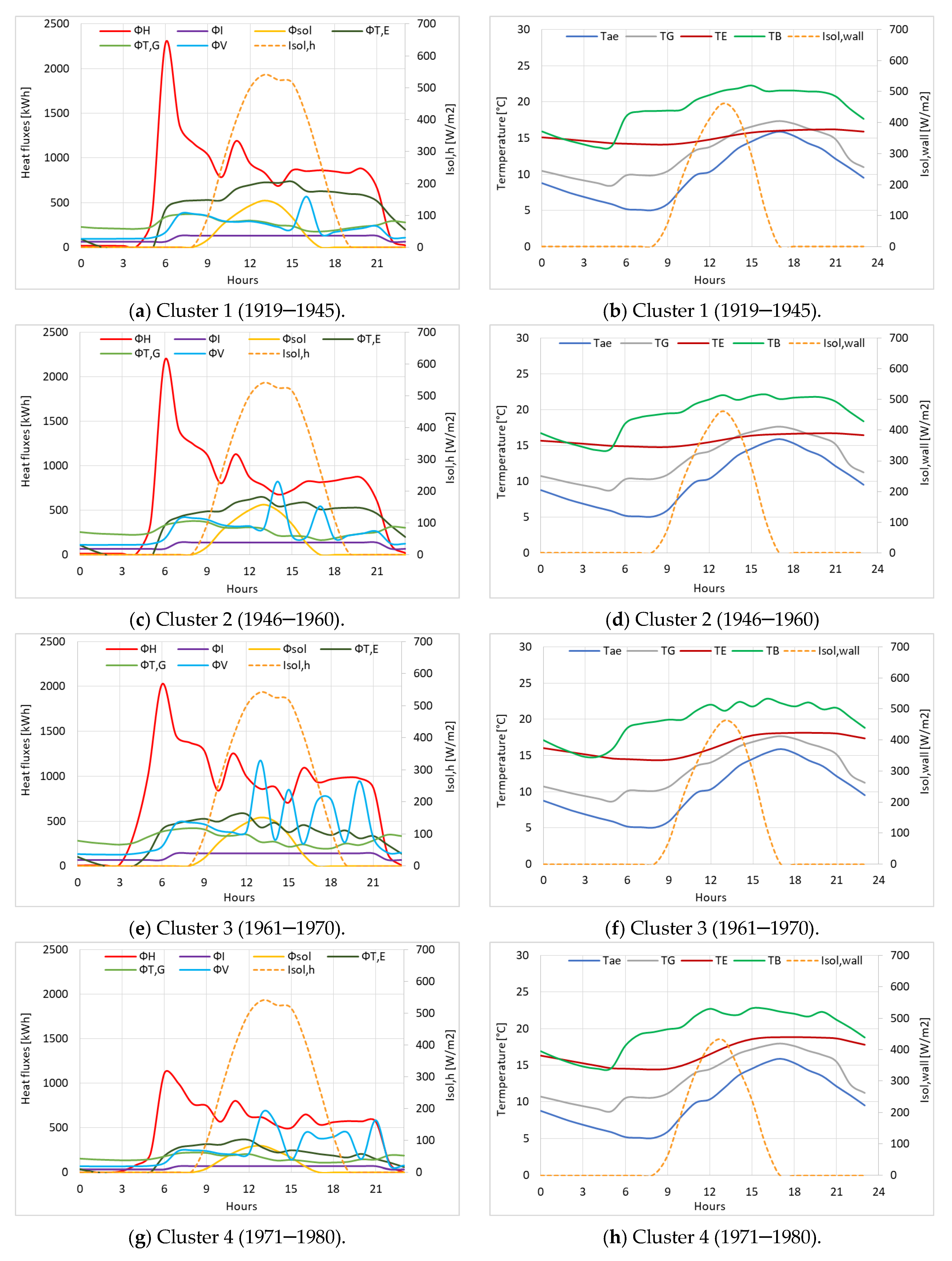
Figure 9.
Heat flux components and building temperatures (with a variable number of air changes per hour and windows opening) for a typical day: October 24th 2013, with a Tae = 16.3 °C (clusters with solid lines and buildings with dashed lines for the three construction periods).
Figure 9.
Heat flux components and building temperatures (with a variable number of air changes per hour and windows opening) for a typical day: October 24th 2013, with a Tae = 16.3 °C (clusters with solid lines and buildings with dashed lines for the three construction periods).

Figure 10.
Positive and negative heat flux contributions with constant ventilation (ach = 0.5 h−1) for the typical monthly days (Tae,day), distinguishing by clusters (c1, c2, c3, c4).
Figure 10.
Positive and negative heat flux contributions with constant ventilation (ach = 0.5 h−1) for the typical monthly days (Tae,day), distinguishing by clusters (c1, c2, c3, c4).

Figure 11.
Building temperatures, TB, with an ach = 0.5 h−1 (solid lines), with a variable ach during the daytime (0.62 h−1) and nighttime (0.3 h−1) (dashed line), and with a variable ach plus window openings (dotted lines) for four typical days (clusters of the four construction periods).
Figure 11.
Building temperatures, TB, with an ach = 0.5 h−1 (solid lines), with a variable ach during the daytime (0.62 h−1) and nighttime (0.3 h−1) (dashed line), and with a variable ach plus window openings (dotted lines) for four typical days (clusters of the four construction periods).

Figure 12.
Correlations between the TB and Tsol-air throughout the daytime from 6 a.m. to 9 p.m. (left column): TB and Tae during the nighttime, from 10 p.m. to 5 a.m. (right column). Distinguishing constant (a, b) and variable ventilation (c, d) and variable ventilation with window openings (e, f).

Figure 13.
Comparison between simulated and measured typical daily thermal consumptions, distinguishing ach = 0.5 h−1 (in orange), ach = 0.62 h−1 during the daytime, ach = 0.3 h−1 during the nighttime (in grey), and a variable ach with window openings (in blue).
Figure 13.
Comparison between simulated and measured typical daily thermal consumptions, distinguishing ach = 0.5 h−1 (in orange), ach = 0.62 h−1 during the daytime, ach = 0.3 h−1 during the nighttime (in grey), and a variable ach with window openings (in blue).
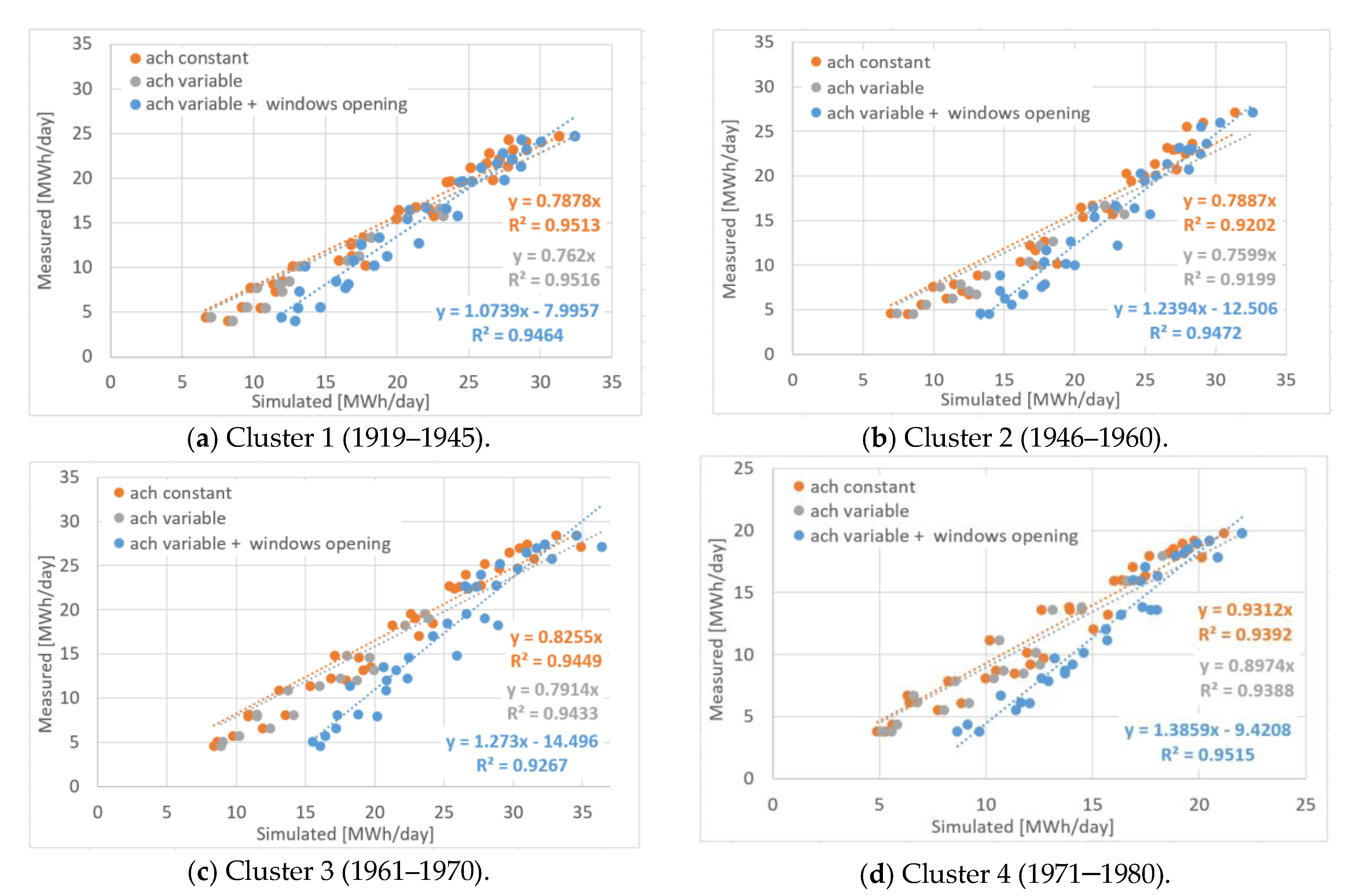
Figure 14.
Example of urban-scale energy tools: 3D city model; building attributes; energy, GHG emissions, and comfort estimation.
Figure 14.
Example of urban-scale energy tools: 3D city model; building attributes; energy, GHG emissions, and comfort estimation.
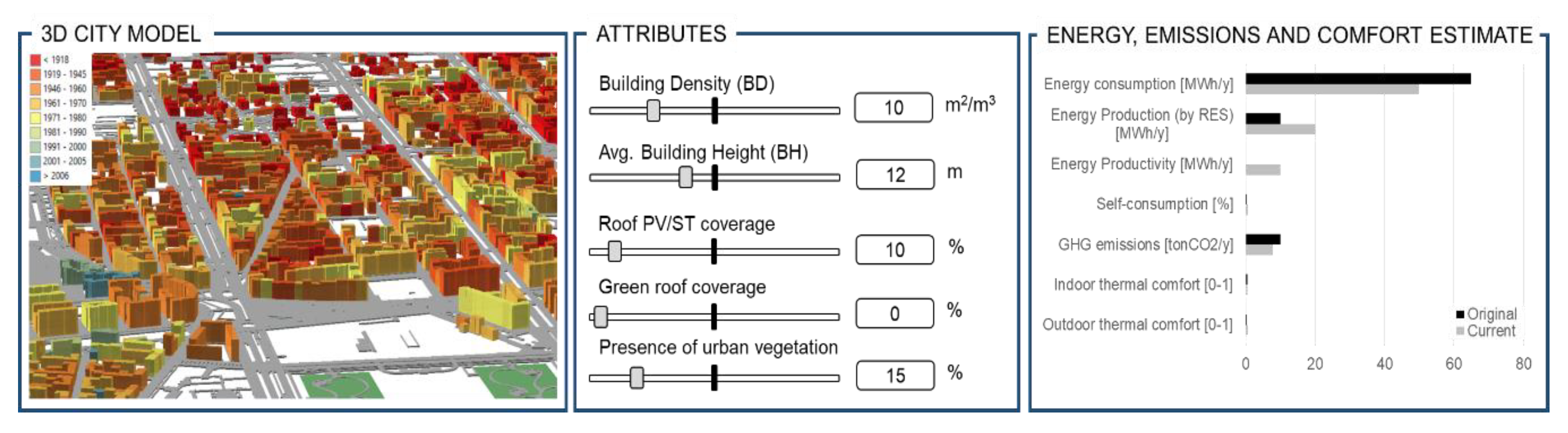
Table 1.
Impacts of energy on resilience in cities [19].
Table 1.
Impacts of energy on resilience in cities [19].
| Environment | Greenhouse gas emissions (GHG) emissions:
|
| Economy | Energy price fluctuations:
|
| Society | Disruptions of energy supply by disasters and critical events:
|
| Governance | Energy governance is affected by various factors:
|
Table 2.
Main input data of buildings and urban morphology characteristics.
| Input data | Source | GIS tool | Scale | |
|---|---|---|---|---|
| Known data | Net and gross area, usable area, heated volume, dispersing surfaces (geometric characteristics) | Municipal Technical Map | Calculate geometry | Building |
| Period of construction, type of user (typological characteristics) | Municipal Technical Map | Select by attributes | Building | |
| Type of roof | Municipal Technical Map, DSM, orthophotos | Aspect, Slope, Solar radiation | Building | |
| Solar exposition | Municipal Technical Map, Digital Surface Model (DSM) | Calculate Polygon Main Angle | Building/Urban | |
| Sky view factor | Municipal Technical Map, DSM | Relief Visualization Toolbox software | Urban | |
| Height-to-distance ratio | Building footprints | Generate near table | Urban | |
| Weather data | ARPA and Politecnico di Torino weather stations | Select by attributes | District | |
| Hypothesized data | Percentage of transparent envelope | National Ministerial Decree of July 5th 1975 (in Italian) | Calculate geometry, Join by attributes | Building |
| Thermal transmittance, resistance, system efficiency | ISO 52016-1:2017, ISO 52017-1:2017, UNI-TR 11552:2014, [36] | Join by attributes | Building | |
| Thermal capacity | ISO 13786:2018, UNI-TR 11552:2014 and UNI 11300-1:2014 | Calculate geometry, Join by attributes | Building |
Table 3.
Thermal transmittances and resistances of the building elements and the TSs (E and G).
| Building Element | 1919–1945 | 1946–1960 | 1961–1970 | 1971–1980 | ||||||||
|---|---|---|---|---|---|---|---|---|---|---|---|---|
| U | 1/2∙Rk+Rse | 1/2∙Rk+Rsi | U | 1/2∙Rk+Rse | 1/2∙Rk+Rsi | U | 1/2∙Rk+Rse | 1/2∙Rk+Rsi | U | 1/2∙Rk+Rse | 1/2∙Rk+Rsi | |
| Slab in cellar | 0.79 | 0.63 | 0.62 | 0.81 | 0.65 | 0.77 | 0.61 | 0.83 | ||||
| Slab in attic | 1.76 | 0.28 | 1.35 | 0.37 | 1.49 | 0.34 | 1.35 | 0.37 | ||||
| Wall | 1.35 | 0.41 | 0.32 | 1.18 | 0.47 | 0.38 | 1.13 | 0.49 | 0.40 | 1.04 | 0.53 | 0.44 |
| Envelope (E) | 1.32 | 0.42 | 0.33 | 1.11 | 0.50 | 0.41 | 1.11 | 0.50 | 0.41 | 1.02 | 0.54 | 0.45 |
| Glazing (G) | 4.75 | 0.15 | 0.06 | 4.40 | 0.16 | 0.07 | 4.90 | 0.15 | 0.06 | 4.57 | 0.15 | 0.06 |
Values of thermal transmittances U are expressed in Wm−2K−1, and the thermal resistances R are in m2KW−1.
Table 4.
Thermal capacities of the building elements and thermodynamic systems (E, G, B).
| Building elements | <1945 | 1946–1960 | 1961–1970 | >1971 |
|---|---|---|---|---|
| Slab in cellar | 317,867 | |||
| Slab in attic | 434,400 | |||
| Wall | 574,560 | 574,560 | 231,000 | 191,520 |
| Envelope (E) | 497,888 | 503,490 | 282,871 | 242,030 |
| Glazing (G) | 7314 | |||
| Building (B): air, furniture and internal partitions | 30,496 * | |||
Values of the thermal capacities are expressed in Jm−2K−1 (per m2 of envelope area). * The reference area [m2] for the building (B) is its net heated surface and not the envelope area.
Table 5.
Cluster characteristics.
| Data | Cluster 1 | Cluster 2 | Cluster 3 | Cluster 4 |
|---|---|---|---|---|
| Period of construction | 1919–1945 | 1946–1960 | 1961–1970 | 1971–1980 |
| No. of buildings | 27 | 32 | 22 | 11 |
| Gross heated volume [m3] | 131,219 (−9%) * | 140,014 (−2%) * | 159,195 (+11%) * | 91,909 (−36%) * |
| Net heated floor [m2] | 37,983 | 40,634 | 41,816 | 25,066 |
| DH consumption [kWh/m3/y] | 29.20 | 27.48 | 26.88 | 21.21 |
| CE [MJ/K] | 23,884 | 25,996 | 10,896 | 5980 |
| CG [MJ/K] | 46 | 50 | 48 | 28 |
| CB [MJ/K] | 1262 | 1463 | 1403 | 799 |
| No. of dwelling units | 494 | 504 | 506 | 240 |
| Heated surface/unit [m2] | 93.31 | 91.13 | 93.46 | 97.06 |
| System efficiency [-] | 0.783 | 0.783 | 0.794 | 0.816 |
* percentage with respect to the average volume of buildings in the three first clusters.
Table 6.
Typical days of a heating season.
| Date 1. | Tae [°C] | Isol,d [Wh/m2/d] | hsol [h] | Tsol-air [°C] | Date 2 | Tae [°C] | Isol,d [Wh/m2/d] | hsol [h] | Tsol-air [°C] |
|---|---|---|---|---|---|---|---|---|---|
| 30/01/2014 | 1.70 | 214 | 9.17 | 2.05 | 29/01/2014 | 1.81 | 397 | 9.17 | 2.49 |
| 09/12/2013 | 3.42 | 1232 | 8.67 | 5.24 | 22/11/2013 | 3.70 | 507 | 9.47 | 4.39 |
| 01/01/2014 | 4.33 | 1610 | 9.17 | 6.60 | 27/11/2013 | 4.44 | 1939 | 9.47 | 7.25 |
| 07/02/2014 | 5.17 | 324 | 8.67 | 5.71 | 26/11/2013 | 5.32 | 2077 | 9.47 | 8.37 |
| 22/02/2014 | 6.24 | 1003 | 10.27 | 8.04 | 16/12/2013 | 6.30 | 1644 | 8.67 | 8.64 |
| 07/01/2014 | 7.30 | 1233 | 9.17 | 8.99 | 15/02/2014 | 7.39 | 1860 | 10.27 | 10.36 |
| 15/11/2013 | 8.32 | 370 | 9.47 | 8.89 | 10/01/2014 | 8.69 | 993 | 9.17 | 10.09 |
| 25/02/2014 | 9.21 | 2706 | 8.67 | 15.01 | 18/11/2013 | 9.36 | 169 | 9.47 | 9.58 |
| 21/01/2014 | 9.86 | 1732 | 9.17 | 12.45 | 22/02/2014 | 10.00 | 3633 | 8.67 | 16.46 |
| 04/11/2013 | 11.19 | 1336 | 9.47 | 13.40 | 05/03/2014 | 11.20 | 4015 | 11.73 | 17.23 |
| 08/03/2014 | 12.48 | 4225 | 11.73 | 18.78 | 13/11/2014 | 12.63 | 2151 | 9.47 | 16.33 |
| 15/10/2013 | 12.99 | 1864 | 10.88 | 16.08 | 01/11/2013 | 13.22 | 2027 | 9.47 | 17.00 |
| 06/11/2013 | 14.68 | 2451 | 9.47 | 19.07 | 19/10/2013 | 14.16 | 1020 | 10.88 | 15.90 |
| 18/10/2013 | 15.02 | 2547 | 10.88 | 19.30 | 18/03/2014 | 15.31 | 4488 | 11.73 | 21.89 |
| 31/03/2014 | 16.22 | 5102 | 11.73 | 23.44 | 30/10/2013 | 16.22 | 1205 | 10.88 | 18.11 |
| 28/10/2013 | 17.08 | 1692 | 10.88 | 19.81 | 09/04/2014 | 17.32 | 5774 | 13.28 | 24.37 |
| 08/04/2014 | 17.97 | 2890 | 13.28 | 21.39 | 14/04/2014 | 17.68 | 5754 | 13.28 | 24.57 |
© 2020 by the authors. Licensee MDPI, Basel, Switzerland. This article is an open access article distributed under the terms and conditions of the Creative Commons Attribution (CC BY) license (http://creativecommons.org/licenses/by/4.0/).
Share and Cite
MDPI and ACS Style
Mutani, G.; Todeschi, V.; Beltramino, S. Energy Consumption Models at Urban Scale to Measure Energy Resilience. Sustainability 2020, 12, 5678. https://doi.org/10.3390/su12145678
AMA Style
Mutani G, Todeschi V, Beltramino S. Energy Consumption Models at Urban Scale to Measure Energy Resilience. Sustainability. 2020; 12(14):5678. https://doi.org/10.3390/su12145678
Chicago/Turabian StyleMutani, Guglielmina, Valeria Todeschi, and Simone Beltramino. 2020. "Energy Consumption Models at Urban Scale to Measure Energy Resilience" Sustainability 12, no. 14: 5678. https://doi.org/10.3390/su12145678
Note that from the first issue of 2016, this journal uses article numbers instead of page numbers. See further details here.