HDPE Geomembranes for Environmental Protection: Two Case Studies
by
 , , and
Fernando Luiz Lavoie
1,2,* ,
,
Clever Aparecido Valentin
2 ,
,
Marcelo Kobelnik
2,
Jefferson Lins da Silva
2 and
and
Maria de Lurdes Lopes
3 1
Department of Civil Engineering, Mauá Institute of Technology, 09580-900 São Caetano do Sul, Brazil
2
São Carlos School of Engineering, University of São Paulo-USP, 05508-220 São Paulo, Brazil
3
Department of Civil Engineering, University of Porto, 4099-002 Porto, Portugal
*
Author to whom correspondence should be addressed.
Sustainability 2020, 12(20), 8682; https://doi.org/10.3390/su12208682
Submission received: 3 September 2020
/
Revised: 2 October 2020
/
Accepted: 12 October 2020
/
Published: 20 October 2020
(This article belongs to the Collection Sustainability in Geotechnics: The Use of Environmentally Friendly Materials)
Abstract
:High-density polyethylene (HDPE) geomembranes have been used for different applications in engineering including sanitation, such as landfills and waste liquid ponds. For these applications, the material can be exposed to aging mechanisms as thermal and chemical degradation, even to UV radiation and biological contact, which can degrade the geomembrane and decrease the material’s durability. This paper aims to present an experimental evaluation of two exhumed HDPE geomembranes, the first was used for 2.75 years in a sewage treatment aeration pond (LTE sample) and another was used for 5.17 years in a municipal landfill leachate pond (LCH sample). Physical and thermal analyses were used such as thermogravimetry (TG), differential thermal analysis (DTA), differential scanning calorimetry (DSC) and dynamic mechanic analysis (DMA). The thermogravimetric analyses showed significant changes in the LCH sample’s thermal decomposition probably caused by the interaction reactions between the polymer and the leachate. For the DSC analyses, the behavior seen in the LTE sample was not observed in the LCH sample. In the DMA analyses, the behavior of the LTE sample storage module shows which LCH sample is less brittle. The LTE sample presented low stress cracking resistance and low tensile elongation at break, following the DMA results.
1. Introduction
A geomembrane is a product of the geosynthetics family used as a liner in the environmental protection system. This polymeric product can be manufactured by the industry in different polymers and it is installed in the field. The high-density polyethylene (HDPE) geomembrane is the most used type of geomembrane in the world, especially for landfills and waste liquid ponds. The high chemical and mechanical resistance of HDPE associated with a low permeability coefficient and low cost of production are the advantages of this product [1,2,3,4,5].
For landfill liner applications, the HDPE geomembrane can be exposed to aging mechanisms such as thermal and chemical degradations. Moreover, for slopes, in the installation time, UV radiation exposition occurs. For leachate ponds and liquid waste treatment applications, the product can be exposed to UV radiation and high temperatures, as well as the chemical and biological contact. This set of aging mechanisms can degrade the geomembrane and decrease the material’s durability [6,7,8,9].
The synergic effects of aging mechanisms can significantly reduce the lifetime of the product. A package of additives is incorporated into the resin to protect the polymer and guarantee the long-term service life [10,11]. In general, carbon black (2–3%) is incorporated into the polymeric resin as UV protection and antioxidants and thermostabilizers (0.5–1.0%) as thermal and oxidative protection [12,13,14].
Islam and Rowe [15] carried out a study with high-density polyethylene geomembranes with nominal thicknesses of 1.5, 2.0 and 2.5 mm immersed in synthetic leachate at four temperatures (22, 55, 70 and 85 °C). The authors used the standard oxidative induction time (OIT) test to evaluate the antioxidant depletion of the samples. They understood which samples with thicker thicknesses demand more time to consume the additives. They concluded that the thicker geomembranes have longer service lives.
Research conducted by Rowe et al. [16] studied an HDPE geomembrane sample (1.5 mm of thickness) in contact with four synthetic leachates with different combinations of volatile fatty acids, inorganic nutrients, trace metal solution and surfactant at four temperatures (the lowest was 22 °C and the highest was 85 °C). The Arrhenius modeling was used to analyze the antioxidant depletion of the geomembrane. The four leachates examined were similar in terms of the antioxidant depletion rate, but the faster depletion occurred in acidic and basic leachates.
Rowe et al. [17] evaluated a 2.0 mm thick HDPE geomembrane for 8 to 10 years exposed to synthetic leachate, water and air in some temperature incubations. The sample contained approximately 97% polyethylene, 2.5% carbon black, and trace amounts of antioxidants and heat stabilizers. The synthetic leachate compound was based in the Keele Valley Landfill leachate in Canada. Several properties of the product were investigated, including the antioxidant depletion, stress cracking resistance, melt flow index and surface analysis. Using the Arrhenius Method to predict the durability of the sample, the results showed that the service life of the product can reach more than 50 years at 50 °C, about 300 years at 35 °C and more than 700 years immersed in leachate at 20 °C.
Lodi and Bueno [18] studied HDPE geomembrane samples with thicknesses of 0.8 and 2.5 mm immersed in synthetic leachate and exposed to weathering using the thermogravimetric analysis (TG). The time in both leachate and weathering expositions was 30 months. It was observed that for the 0.8 mm sample, the thermal stability temperature was higher for the exposed samples compared with the fresh (virgin) sample. The 2.5 mm sample was observed at the same behavior, but the difference among the temperatures was lower than in the 0.8 mm sample. It was observed that the carbon black content of these samples was very low compared to the specifications. The authors commented that the use of multiple analysis such as TG, melt flow index (MFI) and oxidative induction time (OIT) can support the degradation analysis for HDPE geomembranes.
Research was conducted by Ewais et al. [19] over 17 years on an HDPE geomembrane immersed in synthetic leachate, water and air at some temperatures. A stress cracking test, OIT test, MFI test and tensile test were used in the analysis. The authors concluded that the losses in the tensile properties and the stress cracking resistance confirm the oxidative degradation in the polymer. The predicted nominal failure estimated was about 18 years at 60 °C for water and about 13 years at 60 °C for leachate.
Reis et al. [20] carried out a huge field study about HDPE geomembranes exposed by the weather in eight different parts of Portugal. The authors noted that for the higher UV indexes regions, the consequences were higher for tensile properties of the samples. Moreover, the exposed geomembranes had changes in other properties, especially in the OIT results.
Antioxidant depletion analysis was carried out by Safari et al. [21] in an exhumed HDPE geomembrane that was 1.5 mm thick after 25 years of operation in a hazardous waste landfill in Canada. The authors used modern HDPE geomembranes to compare it with the exhumed geomembrane. The results showed that the leachate exposure condition could significantly influence the antioxidant depletion because the bottom samples presented higher OIT depletion than the wall samples. For this study, the sample location and, consequently, the exposure condition differences can represent different behaviors of the samples. The OIT (standard) and some HP-OIT (HP—high pressure) values were found to be significantly lower than those of modern virgin geomembranes.
Some studies evaluated the behavior of high-density polyethylene geomembranes immersed in chlorinated solutions showing a huge polymer degradation capacity of this chemical solution. Abdelaal and Rowe [22] immersed an HDPE geomembrane without HALS (hindered amine light stabilizers) in chlorinated water solutions (0.5, 1.0, 2.5 and 5.0 ppm of free chlorine) at 25, 40, 65, 75 and 85 °C for over 3 years. The authors observed that the antioxidant depletion and the stress cracking resistance in a solution of 5.0 ppm were much faster than synthetic leachate. Abdelaal et al. [23] analyzed the behavior of a high-density polyethylene geomembrane with HALS immersed in four chlorinated solutions with concentrations of 0.5–5.0 ppm at different temperatures for over 5 years. According to the authors, the sample degradation occurred quickly after immersion in all concentrations and incubation temperatures, except for the lower temperature (25 °C). Properties such as tensile and stress cracking decreased when the free chlorine concentration was increased. Finally, the authors noted that the behavior of geomembrane samples with and without HALS showed a huge difference for the chlorinated water solution incubation, but the same difference was not noted for other solution incubations.
Therefore, this work evaluated the final conditions of two exhumed geomembrane samples in sanitation applications using thermoanalytical, physical and mechanical analyses to contribute with the knowledge of HDPE geomembrane behavior applied in environmental facilities.
2. Materials and Methods
2.1. Materials
Two different high-density polyethylene geomembrane samples were evaluated exhumed from sanitation construction works. The first sample was exhumed from a sewage treatment aeration pond (called LTE) after 2.75 years of operation. This geomembrane was damaged during the operation, entailing the pond liner exchange. Table 1 presents the typical characteristics of the sewage. Figure 1 shows the sewage pond which presented an HDPE geomembrane with 1.0 mm of nominal thickness. Another sample was exhumed from a municipal landfill leachate pond (called LCH) after 5.17 years of operation. The exhumation of the geomembrane occurred because the site was used for the landfill expansion. Table 2 presents the chemical characteristics of the municipal landfill leachate. Figure 2 shows the landfill leachate pond that presented an HDPE geomembrane with 2.0 mm of nominal thickness. Both construction works are located in Brazil.
2.2. Physical Properties
The thickness [26] was determined by measuring the difference between the dead-weight loading gauge and the geomembrane specimen thickness with 0.001 mm precision, applying a pressure force of 200 ± 0.2 kPa. The carbon black content (CBC) [27] was determined using a muffle furnace at 605 ± 5 °C for 3 min in an aluminum dish by pyrolysis. It had been used for 1 ± 0.1 g of each geomembrane specimen. The masses before and after being burned were determined using an analytical balance with 0.0001 g precision. The measure of density [28] was performed in isopropyl alcohol at 21 ± 0.1 °C, mass sample 1.0 g ± 0.1 g in apparatus that included an analytical balance with 0.0001 g precision and an immersion vessel and a beaker. The melt flow index (MFI) [29] of the studied samples were obtained using a plastometer with a smooth bore 2.095 ± 0.005 mm in diameter and 8000 ± 0.025 mm long. The polymer was extruded with 190 ± 0.08 °C with a deadweight load of 5.0 kg and its mass was measured for 10 min using an analytical balance with 0.0001 g precision.
2.3. Mechanical Properties
Tensile and tear tests were performed using an EMIC Universal Machine, model DL 3000, manufactured by EMIC at São José dos Pinhais, Brazil, with pneumatic grips and a 2-kN load cell. The tensile test was performed using the type IV dog bone specimen with a test speed of 50 mm min−1, which is the speed test indicated for HDPE geomembranes [30]. The tear test was performed using a test specimen which produces tearing in a small area of stress concentration at rates far below those usually encountered in the field. This test uses a test speed of 51 mm min−1 with an initial jaw separation of 25.4 mm [31].
2.4. Stress Cracking (SC) and Oxidative Induction Time (OIT) Properties
The stress cracking test was performed using an equipment manufactured by WT Indústria at São Carlos, Brazil, with a capacity for 20 specimens simultaneously. The test used was the NCTL-SP (notched constant load test-single point) [32]. Moreover, 30% of yield tensile stress was applied at the specimen using a deadweight with a 10 g precision. The specimen was immersed in a solution of 10% Igepal CO 630 and 90% of water at 50 ± 1 °C. A notch of 20% of the specimen thickness with 0.001 mm of precision was taken in each specimen. The rupture sample time (1 s precision) was measured using an electronic device for each specimen.
For measurements of high-pressure oxidative induction time (OIT-HP) [33], DSC equipment, model Q20, manufactured by TA Instruments at New Castle, United States of America, with high-pressure cell Q series DSC Pressure Cell with a sample mass of 5.0 mg was used. The measurements were proceeded in an open aluminum crucible, under a heating rate of 20 °C min−1, with nitrogen gas purge at a constant pressure of 5 Psi, from ambient temperature to 150 °C. After this stage, nitrogen was exchanged for oxygen at a constant pressure of 500 Psi, maintaining the isotherm of 150 °C until the complete sample oxidation.
2.5. Thermal Analysis Methodology
The thermal analysis was used mainly to evaluate the samples’ conditions and observe the possible changes that occurred. The TG/DTG and DTA curves evaluate the thermal stability temperatures. Furthermore, the activation energy of each sample can be obtained. DSC curves can evaluate the glass transition temperature (Tg), crystallization temperature (Tcrist.) and the melting point of each sample. In addition, the DMA curves evaluate the effects precisely of applied stresses and temperatures under the sample, which allows better precision in the data on molecular relaxation. The knowledge of molecular relaxation helps in the analysis of physical changes in the material, providing information on the protection of the polymer, as molecular relaxation makes the material susceptible to a short lifetime.
The samples were evaluated on dynamic mechanic analysis (DMA) equipment, in a flexural mode, using a DMA thermal analyzer, model Q800, manufactured by TA Instruments at New Castle, United States of America. The samples had a dimension of 35 × 13 mm and were performed under a heating rate of 10 °C min−1 with nitrogen purge gas (flow of 50 mL min−1). The oscillation amplitude of 20 mm was used, with a frequency of 1 Hz and a temperature range from −80 to 125 °C.
The thermogravimetry (TG/DTG) and differential thermal analysis (DTA) were performed at an SDT 2960 (TA Instruments, USA) with heating rates of 5, 10, 20 and 30 °C min−1 under carbonic gas and synthetic air purge gases, with a flow of 100 mL min−1. These polymers were evaluated in an α-alumina crucible in a temperature range of 30 to 600 °C. The activation energy was obtained by the Flynn-Wall-Ozawa method using the DTG curves to obtain the data [34,35,36].
In this study, DSC was used to measure the changes in both materials. Measurements were conducted using a DSC1 Stare, manufactured by Mettler Toledo at Columbus, United States of America, with samples of a diameter of 3 mm2 and masses around 7.5 mg to LTE and 15.5 mg to LCH. These samples were performed in the aluminum crucible in the temperature range of −80 to 200 °C. The first step was cooling from 25 to −80 °C, followed by the second step, where the samples were heated from −80 to 200 °C; in the third step, the samples cooled again from 200 to −80 °C; in the fourth step, the sample was heating from −80 to 200 °C and finally, the fifth step, the sample was cooling from 200 to 25 °C. The heating and cooling rate was 30 ºC min−1 under nitrogen purge gas (flow of 50 mL min−1).
3. Results and Discussion
3.1. Physical Evaluations
Table 3 shows the results of exhumed samples’ physical tests. The average values of the thickness are following the minimum values of the GRI-GM13 [37]. The carbon black content values obtained are also according to the GRI-GM13 [37], which determines values between 2–3%. The obtained density values follow the GRI-GM13 [37], which requires a minimum density value of 0.940 g/cm3. According to Telles et al. [38], low MFI values exhibit good stress cracking environmental resistance for HDPE geomembranes. The obtained results showed low MFI values for both tested samples.
3.2. Mechanical Evaluations
Table 4 shows the results of the exhumed samples’ mechanical tests. The tests were conducted only for the machine direction. The samples’ results are according to the GRI-GM13 [37] concerning the minimum values of the tensile break (27 kN m−1 for 1.0 mm of thickness and 53 kN m−1 for 2.0 mm of thickness) and tear resistance (125 N for 1.0 mm of thickness and 249 N for 2.0 mm of thickness). For the analyzed samples, only the LCH sample presented tensile elongation at breaks higher than 700%, which is the minimum value prescribed by GRI-GM13 [37].
3.3. Stress Cracking (SC) and Oxidative Induction Time (OIT) Evaluations
Table 5 shows the results of the stress cracking test (Notched Constant Tensile Load Test–Single Point-NCTL-SP) and the high-pressure oxidative induction time test (OIT-HP). According to the GRI-GM13 [37], the minimum required value for the stress cracking test (NCTL-SP) is 500 h. The LCH sample performed an average value higher than 500 h but presented a high variation in each specimen value tested, two of the five specimens tested obtained values higher than 1000 h, but the other two of the five specimens obtained values less than 200 h. The mean stress cracking value is in agreement with the tensile behavior of this sample. For the other exhumed sample tested, the results showed a low value of stress cracking resistance. The LTE sample, despite having good tensile behavior and an adequate melt flow index, presented unexpected stress cracking results.
The minimum required value for the OIT High-Pressure test, for the GRI-GM13 [37] is 400 min. According to Mueller and Jakob [39], the main function of antioxidants is to prevent initiation of oxidation chain reactions. Antioxidants are more effective over a certain range of temperatures. As an instance, phosphites are more effective at higher temperatures whereas hindered amine light stabilizers (HALS) are effective at ambient temperature. Hindered phenols, however, are used as long-term stabilizers since they are effective over a wide range of temperatures. None of the samples presented OIT-HP values equal to or higher than 400 min. The presence of HALS in the additive package increases the results of the OIT-HP, as this test is performed at 150 °C. Probably none of the samples presented HALS in the additive package. Both samples presented result values lower than 400 min. The LCH sample obtained the highest OIT-HP value of the exhumed samples tested.
3.4. Thermal Analysis Evaluations
3.4.1. Thermogravimetry (TG) and Differential Thermal Analysis (DTA)
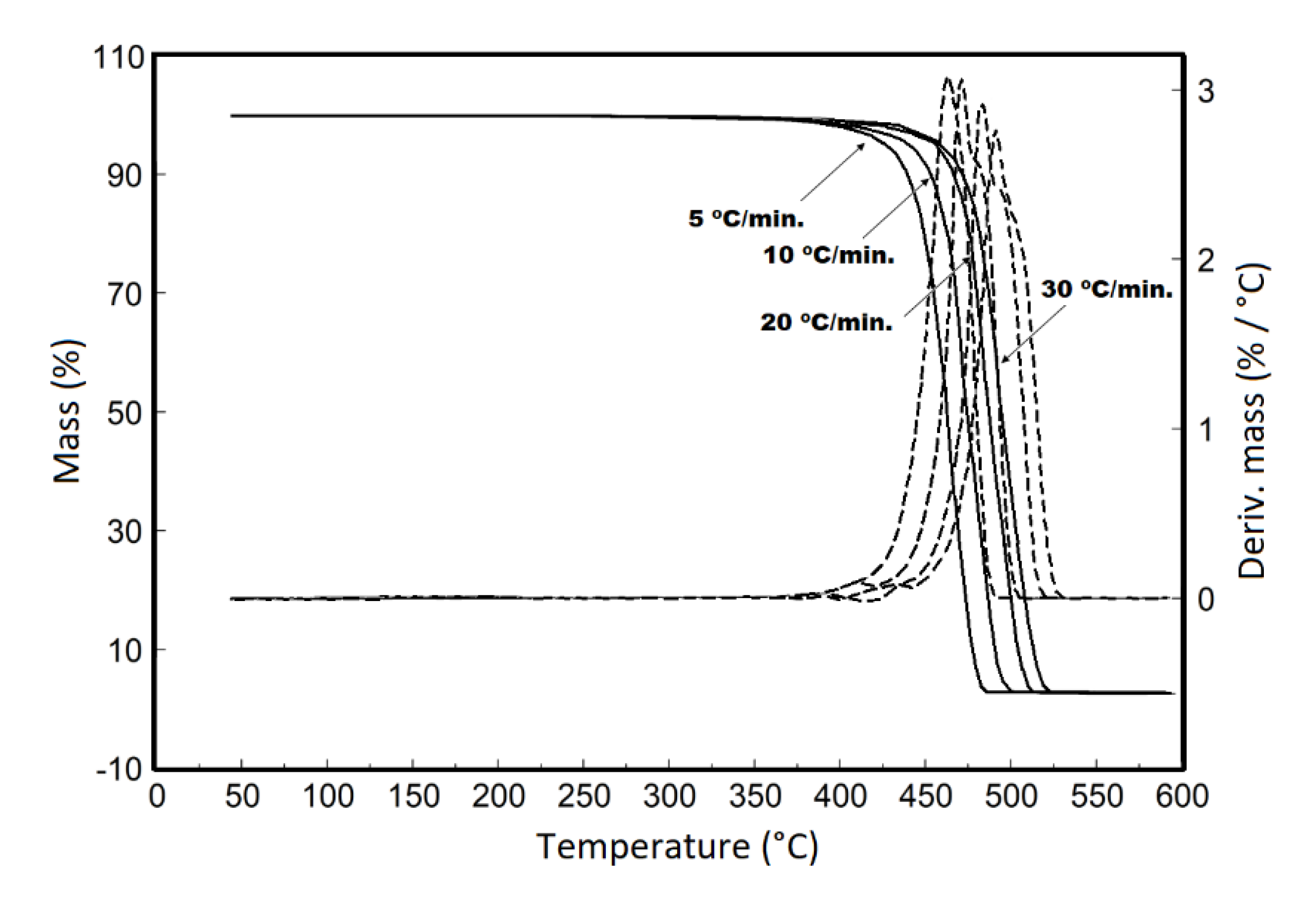
An experiment series was systematically carried out using TG-DTA analysis simultaneously, with heating rates of 5, 10, 20 and 30 °C min−1. The obtained results from both HDPE geomembrane samples are shown in Figure 3, Figure 4, Figure 5 and Figure 6.
Figure 3 shows the TG, DTG and DTA curves of the LTE sample in synthetic air with different heating rates. It was observed that the thermal stability of the LTE sample (TG curves in Figure 3A), which was in contact with the sewage, reached 238 °C for the heating rate of 5 °C and gradually increased to 262 °C for the heating rate of 30 °C. The first sample’s mass variation for the heating rate of 5 °C occurs in one stage only, in the range of 248–369 °C, as seen in the TG curve, whereas in the DTG curve (Figure 3B) only a small deviation from the baseline is seen. The second stage, attributed to the material’s thermal decomposition process, occurs with overlapping reactions, which have presented variations in the intensity of the reactions for the different heating rates, as seen in the TG curves. Furthermore, in the DTG curves it can be observed that with the increase in the heating rate, there is a widening in the decomposition events. For the verification of the mass variations and the respective temperature ranges, the values of each stage are shown in Table 1. For both LTE and LCH samples, at the end of the analyses, the ash formation was observed, which was easily removed from the crucible by a breath. From the DTA curves (Figure 3C), endothermic peaks can be observed at 127, 130, 135 and 140 °C, respectively, for the heating rates of 5, 10, 20 and 30 °C min−1, which were attributed to material melting. This melting point temperature variation is due to the speed of the sample heat absorption, which occurs for different heating rates. Other exothermic peaks are linked to the different stages of the material’s thermal decomposition and, as an effect of the speeds of the different heating rates, the peaks widened.
In the LTE sample analysis, there were no changes in the thermal behavior of the geomembrane, despite the contact of the sample with the sewage for 2.75 years, compared with the results of virgin HDPE geomembrane samples studied by Valentin et al. [40]. However, for the LCH sample evaluation which had been in contact with the leachate for 5.17 years, it was observed that the thermogravimetric behavior presented significant changes in the sample’s thermal decomposition. To ensure this result, two other TG curves were performed in each heating rate to verify the thermal behavior observed once again. Indeed, the other analyses showed that there had been undoubtedly a change in the sample’s thermal behavior due to contact with the leachate. The leachate is a highly concentrated organic substance and this fact added to the 5.17 years of sample exposition can explain the changes in the sample’s thermal behavior. Thus, as seen in the TG curves (Figure 4A), the organic material absorption by the geomembrane probably changed the material’s behavior, causing interaction reactions between the polymer and the leachate. Figure 4A shows that the heating rate of 10 °C min−1 is different from the other curves. In this specific curve, the first mass variation occurs between 259–406 °C and the second mass variation occurs from 406 °C, in two stages, which can be seen in the DTG curve (Figure 4B). The 5 °C heating rate curve shows three stages of mass variation, in the temperature ranges of 248-369, 369–392 and 392–459 °C. For the heating rates of 20 and 30 °C from the second mass variation, the DTG curves are wider, which indicates that the decomposition occurs with overlapping reactions. The mass variation data for each thermal decomposition stage are shown in Table 6.
The obtained results from the DTA curves are shown in Figure 4C for the LCH sample. It can be observed that the first event is an endothermic reaction (without mass variation in the TG/DTG curves), which occurs at temperatures of 127, 132, 138 and 150 °C, for the four heating rates, respectively, representing the samples’ melting point. As both samples (LTE and LCH) were produced with the same type of polymer, the melting point values differ slightly from each other probably due to their different uses of the conditions. The following stages of thermal decomposition are exothermic reactions for the four heating rates. The heating rate of 5 °C min−1 showed a sharp peak in the second stage of thermal decomposition, which is attributed to a sample combustion reaction. In addition, as with the LTE sample, it can be observed that with the increase in the heating rate, there is a widening effect of the exothermic reactions due to the overlapping reactions.
The TG/DTG curves in a non-isothermal condition, shown in Figure 5 and Figure 6, in carbon dioxide purge gas, with the analyses at different heating rates, were used to obtain the kinetic data of the LTE and LCH samples, respectively.
For the LTE sample, as seen in Figure 5, there was no change in mass between the initial temperature and 376 °C for the analysis in the heating rate of 5 °C, while for the other heating rates, the values were: 381 °C (10 °C min−1), 405 °C (20 °C min−1) and 410 °C (30 °C min−1). The mass variation values are shown in Table 1. It can also be observed that the TG curves show similarities since the beginning of the thermal decomposition behavior, with the presence of a shoulder at the beginning of the decomposition reaction and later homogeneity during the thermal decomposition.
For the LCH sample, as seen in Figure 6, the geomembrane thermal stability occurs up to the following temperatures and respective heating rates: 378 °C (5 °C min−1), 383 °C (10 °C min−1), 387 °C (20 °C min−1) and 401 °C (30 °C min−1). The thermal decomposition process showed that at the beginning of the reaction, a small shoulder was formed and then a thermal decomposition occurred. During the main decomposition process, a shoulder formation also occurred in the DTG curves, except for the heating rate of 5 °C min−1 which was attributed to overlapping decomposition reactions.
At the end of the thermal decomposition reaction, for the analysis of both samples, the presence of carbonaceous material impregnated in the crucible was observed, which was removed.
The activation energy values are shown in Table 2, which presents the intervals used to obtain the kinetic values for the analyses in carbonic gas and synthetic air, except for the LCH sample. This sample presented an altered decomposition behavior, that is, the heating rates did not show homogeneous displacement among them, as seen in the other analyses. Therefore, this sample was not analyzed in the synthetic purge gas.
Figure 7 shows the behavior of the activation energy during thermal decomposition. For the analysis of the LTE sample in synthetic air, it can be observed that the activation energy has a lower value than the analysis carried out on carbon dioxide and shows that there is a gradual decrease. This shows that the thermal decomposition of the material occurred using the purge gas during the reaction, that is, an oxidation reaction occurs between the oxygen present in the synthetic air and the polymer. For the LTE sample reaction in carbonic gas, it can be observed that the initial value of its activation energy is close to the synthetic air analysis. However, there is a gradual increase in the activation energy. This gradual increase indicates which decomposition occurs due to the increase in temperature, considering that carbonic gas is inert. Likewise, for the LCH sample, in addition to having initial activation energy values higher than those of the LTE sample, the same behavior of a gradual increase in activation energy also occurs. The HDPE activation energy values under a nitrogen atmosphere were reported by Valentin et al. [40]. These authors showed that the activation energies values were similar to those obtained in this work, however, the authors did not proceed with any evaluation in another atmosphere.
Additionally, the correlation coefficient values (Table 7) show a linear pattern for the analyzed samples, which shows that the kinetic data follow the same behavior trend.
3.4.2. Differential Scanning Calorimetry (DSC)
Figure 8 and Figure 9 show, respectively, the LTE and LCH samples analyses under heating and cooling conditions performed to verify the materials’ transitions.
Figure 8A shows that during the first cooling there was a decrease in the LTE sample heat flow, which coincides with the baseline of the second cooling between 5 to −28 °C. The first heating of the sample (Figure 8B) shows that there had been a change in the baseline of the curve between −55 to −25 °C. For the second cooling, there was a heat flow decrease in the range of −28 to −40 °C, which is attributed to a difference in the heat capacity of the sample. However, in the second and third heating, there was an inverse behavior, that is, there was an increase in the material’s heat flow. These changes in the sample’s heat flow occurred due to the behavior of the material’s molecules, which during cooling, the polymer molecules undergo contraction due to low temperature, getting closer to one another, and consequently changing the sample dimensions. During heating, the molecules tend to distance themselves from each other, and thus, the heat capacity changes, causing the accumulated energy to be released [41]. In contrast, in the first heating, the material melted and then there was a crystallization, where there is a molecular reorganization and a temperature decrease. Then, the molecular structure experiences a decrease in the heat flow between −25 and −39 °C, which shows an energy loss that corresponds to a material’s molecular approximation. As the material was heated and recrystallized again, there was an even more random molecular reorganization, which causes the change in the heat flow. When reheating this sample again, in the second heating (Figure 8B) there is an increase in the sample’s heat flow, and then the new fusion, which has a wider peak area than the first fusion. When recrystallizing again, as seen in the third cooling, the peak is also smaller and wider. However, as seen, there was a small change in the baseline between −4 to −19 °C. Finally, in the third heating, there was an overlap with the event observed in the second cooling, attributed to the molecular distance.
For the LCH sample, the behavior seen in the LTE sample was not observed. It indicates that there was probably an effect of leachate in the sample, causing a change in the heat flow. As seen in Figure 9A, the first cooling and the first heating have the same behavior observed for the LTE sample. After the melting and the first crystallization, a slight change in the baseline is seen in the second cooling (17 to 8 °C) and the third cooling (7 to −2 °C), both in agreement with what is seen in the third cooling of the LTE sample. It is important to note that during the heating of this sample, there was no change in the material’s baseline between (−54 to −16 °C). Thus, it can be reaffirmed that the effect caused on the DSC curve for the LCH sample is attributed to the presence of leachate molecules, which altered the material’s behavior after the melting process.
3.4.3. Dynamic Mechanical Analysis (DMA)
DMA was used to track changes in the molecular relaxation of the materials, to learn whether these changes were a function of the time in operation and an indication of the material’s degradation, and to learn about the effects of leachate and sewage on the material. DMA analyses usually have different modules, which allow a better characterization of the material, that is, the material’s capacity to store energy (storage modulus), its capacity to lose energy (loss modulus) and the proportion of these effects (tan-δ), which is called damping (damping factor) [42].
Figure 10 shows the DMA analysis under nitrogen purge gas, at a range temperature of −80 to 120 °C for both samples, where it is possible to verify that both samples have different behavior between each other. The temperature range utilized in this analysis is situated above the glass transition temperature, which is a region of high hardness and therefore, the information obtained from the temperature of −80 °C refers to the transition region performed in this work [43]. The behavior of the LTE sample storage module (Figure 10A) shows that this sample has a higher value than the LCH sample, which means that the LCH sample is less brittle, that is, more elastic. The basic definition of the storage module is given as a measure of the mechanical energy that the material is capable of storing, in the form of potential or elastic energy [44]. This result shows that the potential energy of the LTE sample decreases gradually until the temperature of 32 °C, and after this temperature, this sample increases its potential energy again until the temperature of 78 °C. This effect is attributed to the simultaneous effect of raising the temperature and the interaction of the geomembrane polymer with molecules from the sewage which were impregnated in the geomembrane, which causes an increase in stiffness (becomes less elastic). The same effect is observed for the LCH sample, but to a lesser degree. The expected trend would be an increase in the elasticity of the material and a consequent decrease in stiffness.
These results show that the geomembranes’ contact with the sewage and leachate caused the alteration in elastic potential, which is attributed to the molecular interaction in the structure of the polymeric matrix. Furthermore, from temperatures of 72 °C for the LTE sample and 85 °C for the LCH sample, both samples tend to increase viscosity since the increase in temperature leads to the melting stage, that is, the polymer chains start to have a greater movement due to the increase in the temperature with loss of stored energy, until the consequent fusion.
The loss module (E″) is shown in Figure 10B, which shows that the LTE sample has a much higher curve behavior than the LCH sample curve in the same temperature range (32 to 125 °C). This information indicates that the LTE sample, when dissipating the energy stored in this interval, shows that its elasticity decreases again, while the LCH sample has a constant behavior, showing variations in different temperature ranges [45].
In Figure 10C, tan-δ is shown, which is a relationship between the material’s elastic/stiffness behavior [42,43]. As both materials are stiffer at low temperatures, tan-δ tends to increase with the temperature increasing. Thus, for the LTE sample at the temperature of 32 °C a peak of tan-δ, there was a peak in the decrease in the material’s stiffness and after this temperature there was a decrease in the tan-δ, indicating an increase in stiffness. For the LCH sample there was the same behavior but with the tan-δ peak at 63 °C, which corresponds to the temperature at which is the value of the lowest potential energy of this sample (Figure 10A), that is, after this temperature, this sample increases its potential energy up to 82 °C. As with the LTE sample, there was an increase in the LCH stiffness, and therefore, the tan-δ peak (63 °C) corresponds to this situation. Tan-δ decreases with increasing stiffness, that is, if the material is at a constant stiffness, tan-δ will be constant (will have a zero value) [46,47].
4. Conclusions
This paper analyzed two HDPE geomembrane samples exposed to different sanitation environments. The interaction and the aging of the studied samples may be different, not only in relation to the different fluids but also in relation to the different geomembranes’ thicknesses and to the different exposed periods of time. The samples presented some similarities and some differences in their behaviors. The thermogravimetric analyses showed significant changes in the LCH sample’s thermal decomposition. The organic material absorption by the geomembrane probably changed the material’s behavior, causing interaction reactions between the polymer and the leachate. In the LTE sample analysis, no changes were observed in the geomembrane thermal behavior.
In the kinetic evaluation, for the analysis of the LTE sample, with a synthetic air purge gas, it can be observed that the activation energy has a lower value than the analysis carried out in carbon dioxide. For the LTE sample reaction in carbonic gas, it can be observed that the initial value of its activation energy is close to the synthetic air analysis. However, there is a gradual increase in the activation energy. This gradual increase indicates which decomposition occurs due to the increase in temperature, considering that carbonic gas is inert. The LCH sample presented an altered decomposition behavior, that is, the heating rates did not show homogeneous displacement among them, as seen in the other analyses.
For the DSC analyses, the behavior seen in the LTE sample was not observed in the LCH sample. It indicates that probably there was an effect of leachate in the sample, causing a change in the heat flow. For the LCH sample, after the melting and the first crystallization, a slight change in the baseline is seen in the second cooling and the third cooling, both in agreement with what is seen in the third cooling of the LTE sample. It is important to note that during the heating of this sample, there was no change in the material’s baseline. Thus, it can be reaffirmed that the effect caused on the DSC curve for the LCH sample is attributed to the presence of leachate molecules, which altered the material’s behavior after the melting process.
The DMA analyses showed different behaviors between the samples. The behavior of the LTE sample storage module shows that this sample has a higher value than for the LCH sample, which means that the LCH sample is less brittle, that is, more elastic. These results follow the physical results, because the LTE sample presented low stress cracking resistance and low tensile elongation at break. By analyzing the loss module, can be observed that the LTE sample, when dissipating the energy stored in this interval, shows that its elasticity decreases again, while the LCH sample has a constant behavior, showing variations in different temperature ranges. Both samples presented the similar behavior in the tan-δ analysis, but the temperature at which is the value of the lowest potential energy was different for the samples. All polymeric materials, with rare exceptions, are elastic. The molecular interaction will determine the elasticity of the material, that is, the greater the molecular disorganization, the more amorphous the material will be.
For future studies, we recommended obtaining and characterizing the virgin sample and monitoring the exposed samples during the exposition at predetermined times. Besides, to characterize the fluids in contact with the geomembranes and to monitor their properties along the exposed time is recommended.
Author Contributions
Conceptualization, F.L.L., C.A.V., J.L.d.S. and M.d.L.L.; methodology, M.K.; validation, F.L.L., C.A.V. and M.K.; formal analysis, C.A.V. and M.K..; investigation, F.L.L., C.A.V. and M.K.; resources, F.L.L. and M.K.; writing—original draft preparation, F.L.L., C.A.V. and M.K.; writing—review and editing, F.L.L., C.A.V., J.L.d.S. and M.d.L.L.; visualization, F.L.L. and C.A.V.; supervision, F.L.L.; project administration, J.L.d.S. All authors have read and agreed to the published version of the manuscript.
Funding
This research received no external funding.
Conflicts of Interest
The authors declare no conflict of interest.
References
- Rollin, A.R.; Rigo, J.M. Geomembranes—Identification and Performance Testing, 1st ed.; Chapman and Hall: London, UK, 1991. [Google Scholar]
- Palmeira, E.M. Geossintéticos em Geotecnia e Meio Ambiente, 1st ed.; Oficina de Textos: São Paulo, Brazil, 2018. [Google Scholar]
- Koerner, R.M. Designing with Geosynthetics, 5th ed.; Prentice Hall: Upper Saddle River, NJ, USA, 2005. [Google Scholar]
- Scheirs, J. A Guide to Polymeric Geomembranes: A Practical Approach, 1st ed.; Wiley: London, UK, 2009. [Google Scholar]
- Vertematti, J.C. Manual Brasileiro de Geossintéticos, 2nd ed.; Blücher: São Paulo, Brazil, 2015. [Google Scholar]
- Rowe, R.K.; Sangam, H.P. Durability of HDPE Geomembranes. Geotext Geomembr. 2002, 20, 77–95. [Google Scholar] [CrossRef]
- Kay, D.; Blond, E.; Mlynarek, J. Geosynthetics durability: A polymer chemistry issue. In Proceedings of the 57th Canadian Geotechnical Conference, Quebec, QC, Canada, 24–26 October 2004. [Google Scholar]
- Rowe, R.K.; Abdelaal, F.B.; Brachman, R.W.I. Antioxidant depletion of HDPE geomembrane with sand protection layer. Geosynth. Int. 2013, 20, 73–89. [Google Scholar] [CrossRef]
- Koerner, G.R.; Hsuan, Y.G.; Koerner, R.M. The durability of geosynthetics. In Geosynthetics in Civil Engineering, 1st ed.; Sarsby, R.W., Ed.; Woodhead Published Limited: Cambridge, UK, 2007; pp. 36–65. [Google Scholar]
- Hsuan, Y.G.; Koerner, R.M. The single point-notched constant tension load test: A quality control test for assessing stress crack resistance. Geosynth. Int. 1995, 2, 831–843. [Google Scholar] [CrossRef]
- Hsuan, Y.G.; Koerner, R.M. Antioxidant depletion lifetime in high density polyethylene geomembranes. J. Geotech. Geoenviron. 1998, 124, 532–541. [Google Scholar] [CrossRef]
- Ewais, A.M.R.; Rowe, R.K.; Scheirs, J. Degradation behaviour of HDPE geomembranes with high and low initial high-pressure oxidative induction time. Geotext. Geomembr. 2014, 42, 111–126. [Google Scholar] [CrossRef]
- Lodi, P.C.; Bueno, B.S.; Vilar, O.M. The Effects of Weathering Exposure on the Physical, Mechanical, and Thermal Properties of High-density Polyethylene and Poly (Vinyl Chloride). Mater. Res. 2013, 16, 1331–1335. [Google Scholar] [CrossRef] [Green Version]
- Rowe, R.K.; Ewais, A.M.R. Ageing of exposed geomembranes at locations with different climatological conditions. Can. Geotech. J. 2015, 52, 326–343. [Google Scholar] [CrossRef] [Green Version]
- Islam, M.Z.; Rowe, R.K. Effect of HDPE geomembrane thickness on the depletion of antioxidants. In Proceedings of the 60th Canadian Geotechnical Conference and the 8th Joint CGS/IAH-CNC Groundwater Conference, Ottawa, ON, Canada, 21–24 October 2007. [Google Scholar]
- Rowe, R.K.; Islam, M.Z.; Hsuan, Y.G. Leachate chemical composition effects on OIT depletion in an HDPE geomembrane. Geosynth. Int. 2008, 15, 136–151. [Google Scholar] [CrossRef] [Green Version]
- Rowe, R.K.; Rimal, S.; Sangam, H. Ageing of HDPE geomembrane exposed to air, water and leachate at different temperatures. Geotext. Geomembr. 2009, 27, 137–151. [Google Scholar] [CrossRef]
- Lodi, P.C.; Bueno, B.S. Thermo-gravimetric Analysis (TGA) after Different Exposures of High Density Polyethylene (HDPE) and Poly Vinyl Chloride (PVC) Geomembranes. Electron. J. Geotech. Eng. 2012, 17, 3339–3349. [Google Scholar]
- Ewais, A.M.R.; Rowe, R.K.; Rimal, S.; Sangam, H.P. 17-year elevated temperature study of HDPE geomembrane longevity in air, water and leachate. Geosynth. Int. 2018, 25, 525–544. [Google Scholar] [CrossRef]
- Reis, R.K.; Barroso, M.; Lopes, M.G. Evolução de cinco geomembranas expostas a condições climáticas em Portugal durante 12 anos. GEOTECNIA 2017, 141, 41–58. [Google Scholar] [CrossRef]
- Safari, E.; Rowe, R.K.; Markle, J. Antioxidants in an HDPE geomembrane used in a bottom liner and cover in a PCB containment landfill for 25 years. In Proceedings of the Pan Am CGS Geotechnical Conference, Toronto, ON, Canada, 2–6 October 2011. [Google Scholar]
- Abdelaal, F.B.; Rowe, R.K. Degradation of an HDPE geomembrane without HALS in chlorinated water. Geosynth. Int. 2019, 26, 354–370. [Google Scholar] [CrossRef]
- Abdelaal, F.B.; Morsy, M.S.; Rowe, R.K. Long-term performance of a HDPE geomembrane stabilized with HALS in chlorinated water. Geotext Geomembr. 2019, 47, 815–830. [Google Scholar] [CrossRef]
- Leite, A.F.R.; Ligeiro, L.P.M. Características, Tratamento e Potencial Utilização de Esgoto Produzido em Shopping Centers: Estudo de caso do Catarina Fashion Outlet. Master’s Thesis, University of São Paulo, São Paulo, Brazil, 2017. [Google Scholar]
- Química Pura Laboratório de Análises Químicas. Relatório de Ensaios nº 49808/18. Giruá, Rio Grande do Sul, Brazil. 2018. [Google Scholar]
- ASTM (American Society for Testing and Materials). ASTM D 5199 Standard Test Methods for Measuring the Nominal Thickness of Geosynthetics; ASTM: West Conshohocken, PA, USA, 2012; p. 4. [Google Scholar]
- ASTM (American Society for Testing and Materials). ASTM D 4218 Standard Test Method for Determination of Carbon Black Content in Polyethylene Compounds by the Muffle-Furnace Technique; ASTM: West Conshohocken, PA, USA, 2020; p. 4. [Google Scholar]
- ASTM (American Society for Testing and Materials). ASTM D 792 Standard Test Methods for Density and Specific Gravity (Relative Density) of Plastics by Displacement; ASTM: West Conshohocken, PA, USA, 2013; p. 6. [Google Scholar]
- ASTM (American Society for Testing and Materials). ASTM D 1238 Standard Test Methods for Melt Flow Rates of Thermoplastics by Extrusion Plastometer; ASTM: West Conshohocken, PA, USA, 2013; p. 16. [Google Scholar]
- ASTM (American Society for Testing and Materials). ASTM D 6693 Standard Test Methods for Determining Tensile Properties of Nonreinforced Polyethylene and Nonreinforced Flexible Polypropylene Geomembranes; ASTM: West Conshohocken, PA, USA, 2015; p. 5. [Google Scholar]
- ASTM (American Society for Testing and Materials). ASTM D 1004 Standard Test Methods for Tear Resistance (Graves Tear) of Plastic Film and Sheeting; ASTM: West Conshohocken, PA, USA, 2013; p. 4. [Google Scholar]
- ASTM (American Society for Testing and Materials). ASTM D 5397 Standard Test Method for Evaluation of Stress Crack Resistance of Polyolefin Geomembranes Using Notched Constant Tensile Load Test; ASTM: West Conshohocken, PA, USA, 2020; p. 7. [Google Scholar]
- ASTM (American Society for Testing and Materials). ASTM D 5885 Standard Test Method for Oxidative Induction Time of Polyolefin Geosynthetics by High-Pressure Differential Scanning Calorimetry; ASTM: West Conshohocken, PA, USA, 2017; p. 5. [Google Scholar]
- Dias, D.S.; Crespi, M.S.; Ribeiro, C.A.; Kobelnik, M. Evaluation by thermogravimetry of the interaction of the poly(ethylene terephthalate) with oil-based paint. Eclét. Quím. 2015, 40, 77–85. [Google Scholar] [CrossRef]
- Dias, D.S.; Crespi, M.S.; Kobelnik, M.; Ribeiro, C.A. Calorimetric and SEM studies of polymeric blends of PHB-PET. J. Anal. Calorim. 2009, 97, 581–584. [Google Scholar] [CrossRef]
- Lima, J.S.; Kobelnik, M.; Ribeiro, C.A.; Capela, J.M.V.; Crespi, M.S. Kinetic study of crystallization of PHB in presence of hydroxy acids. J. Anal. Calorim. 2009, 97, 525–528. [Google Scholar] [CrossRef]
- GRI (Geosynthetic Research Institute). GRI—GM13 Test Methods, Test Properties and Testing Frequency for High Density Polyethylene (HDPE) Smooth and Textured Geomembranes; GRI: Folsom, PA, USA, 2019; p. 11. [Google Scholar]
- Telles, R.W.; Lubowitz, H.R.; Unger, S.L. Assessment of Environmental Stress Corrosion of Polyethylene Liners in Landfills and Impoundments, 1st ed.; U.S. EPA: Cincinnati, OH, USA, 1984.
- Mueller, W.; Jakob, I. Oxidative resistance of high density polyethylene geomembranes. Polym. Degrad. Stab. 2003, 79, 161–172. [Google Scholar] [CrossRef]
- Valentin, C.A.; Silva, J.L.; Kobelnik, M.; Ribeiro, C.A. Thermoanalytical and dynamic mechanical analysis of commercial geomembranes used for fluid retention of leaching in sanitary landfills. J. Anal. Calorim. 2018, 136, 471–481. [Google Scholar] [CrossRef] [Green Version]
- Höhne, G.W.H.; Hemminger, W.F.; Flammersheim, H.J. Differential Scanning Calorimetry, 2nd ed.; Springer: Berlin/Heidelberg, Germany, 2003. [Google Scholar]
- Gabbott, P. Principles and Applications of Thermal Analysis, 1st ed.; Blackwell Publishing Ltd.: Oxford, UK, 2008. [Google Scholar]
- Menard, K.P. Dynamic Mechanical Analysis: A Practical Introduction, 2nd ed.; CRC Press Taylor & Francis Group: Boca Raton, FL, USA, 2008. [Google Scholar]
- Cassu, S.N.; Felisberti, M.I. Comportamento dinâmico-mecânico e relaxações em polímeros e blendas poliméricas. Quim. Nova 2005, 28, 255–263. [Google Scholar] [CrossRef]
- Hatakeyama, T.; Quinn, F.X. Thermal Analysis: Fundamentals and Applications to Polymer Science, 2nd ed.; John Wiley & Sons Ltd.: Baffins Lane Chichester, UK, 1999. [Google Scholar]
- Krongauz, V.V. Diffusion in polymers dependence on crosslink density. Eyring approach to mechanism. J. Anal. Calorim. 2010, 102, 435–445. [Google Scholar] [CrossRef]
- Suceska, M.; Liu, Z.Y.; Sanja Matecic Musanic, S.M.; Fiamengo, I. Numerical modelling of sample–furnace thermal lag in dynamic mechanical analyser. J. Anal. Calorim. 2010, 100, 337–345. [Google Scholar] [CrossRef]
Figure 1.
Sewage treatment aeration pond under operation.

Figure 2.
Municipal landfill leachate pond under demobilization.

Figure 3.
(A) TG curves for LTE sample in the synthetic gas purge, with mass samples around 7.50 mg; (B) DTG curves for the LTE sample in the synthetic gas purge, with mass samples around 7.50 mg; (C) DTA curves for the LTE sample in the synthetic gas purge, with mass samples around 7.50 mg. (all analyses conducted with heating rates of 5, 10, 20 and 30 °C min−1 with the flow of 110 mL min−1 in α-alumina crucible).

Figure 4.
(A) TG curves for LCH sample in synthetic gas purge, with mass samples around 15.50 mg; (B) DTG curves for the LCH sample in synthetic gas purge, with mass samples around 15.50 mg; (C) DTA curves for the LCH sample in synthetic gas purge, with mass samples around 15.50 mg (all analyses conducted with heating rates of 5, 10, 20 and 30 °C min−1 with the flow of 110 mL min−1 in α-alumina crucible).

Figure 5.
LTE sample TG/DTG curves in carbonic purge gas, with mass samples around 7.50 mg, with analyses conducted with heating rates of 5, 10, 20 and 30 °C min−1 with the flow of 110 mL min−1 in α-alumina crucible.
Figure 5.
LTE sample TG/DTG curves in carbonic purge gas, with mass samples around 7.50 mg, with analyses conducted with heating rates of 5, 10, 20 and 30 °C min−1 with the flow of 110 mL min−1 in α-alumina crucible.

Figure 6.
LCH sample TG/DTG curves in carbonic purge gas, with mass samples around 15.50 mg, with analyses conducted with heating rates of 5, 10, 20 and 30 °C min−1 with the flow of 110 mL min−1 in an α-alumina crucible.
Figure 6.
LCH sample TG/DTG curves in carbonic purge gas, with mass samples around 15.50 mg, with analyses conducted with heating rates of 5, 10, 20 and 30 °C min−1 with the flow of 110 mL min−1 in an α-alumina crucible.

Figure 7.
Activation energy versus degree conversion for LTE and LCH samples.

Figure 8.
LTE sample DSC curves with a heating rate of 30 °C min−1 under nitrogen gas purge with the flow of 50 mL min−1 in an aluminum crucible with sample masses around 3.50 mg: (A) heating and (B) cooling.
Figure 8.
LTE sample DSC curves with a heating rate of 30 °C min−1 under nitrogen gas purge with the flow of 50 mL min−1 in an aluminum crucible with sample masses around 3.50 mg: (A) heating and (B) cooling.

Figure 9.
LCH sample DSC curves with a heating rate of 30 °C min−1 under nitrogen gas purge with the flow of 50 mL min−1 in an aluminum crucible with sample masses around 3.50 mg: (A) heating and (B) cooling.
Figure 9.
LCH sample DSC curves with a heating rate of 30 °C min−1 under nitrogen gas purge with the flow of 50 mL min−1 in an aluminum crucible with sample masses around 3.50 mg: (A) heating and (B) cooling.

Figure 10.
DMA curves of LCH and LTE samples with a heating rate of 5 °C min−1 under nitrogen gas purge with a flow of 50 mL min−1: (A) storage modulus, (B) loss modulus and (C) tan delta.
Figure 10.
DMA curves of LCH and LTE samples with a heating rate of 5 °C min−1 under nitrogen gas purge with a flow of 50 mL min−1: (A) storage modulus, (B) loss modulus and (C) tan delta.


Table 1.
Typical characteristics of the sewage [24].
Table 1.
Typical characteristics of the sewage [24].
| Characteristic | Unit | Result |
|---|---|---|
| Fixed Suspension Solids | mg/L | 80 |
| Volatile Suspended Solids | mg/L | 320 |
| Total Suspended Solids | mg/L | 350 |
| Fixed Dissolved Solids | mg/L | 400 |
| Volatile Dissolved Solids | mg/L | 300 |
| Total Dissolved Solids | mg/L | 700 |
| Sedimentable Solids | mg/L | 15 |
| Total solids | mg/L | 1100 |
| pH | - | 6.5–7.5 |
| BOD | mg/L | 100–400 |
Table 2.
Chemical characteristics of the municipal landfill leachate [25].
Table 2.
Chemical characteristics of the municipal landfill leachate [25].
| Characteristic | Unit | Result |
|---|---|---|
| Total alkalinity | mg CaCO3/L | 6912 |
| Calcium | mg/L | 366 |
| Cadmium | mg/L | Not Detected |
| Lead | mg/L | Not Detected |
| Chloride | mg Cl-/L | 3502 |
| Total Coliforms | NMP/100 mL | 8.3 |
| Conductivity | μS/cm | 23,210 |
| BOD | mg O2/L | 775 |
| Iron | mg/L | 11.4 |
| Magnesium | mg/L | 0.165 |
| Mercury | mg/L | Not Detected |
| Nickel | mg/L | 0.230 |
| pH | - | 8.19 |
| Mineral Oils and Greases | mg/L | Not Detected |
Table 3.
Physical test results of exhumed samples.
| Sample | Thickness/(mm) | CBC/(%) | Density/(g/cm3) | MFI/(g/10 min) |
|---|---|---|---|---|
| LTE | 1.001 (±0.038) | 2.49 (±0.47) | 0.959 (±0.001) | 0.4555 (±0.0061) |
| LCH | 2.075 (±0.036) | 2.36 (±0.11) | 0.946 (±0.002) | 0.5008 (±0.0072) |
The standard deviations are shown between brackets. CBC = carbon black content.
Table 4.
Mechanical test results of exhumed samples.
| Sample | Tens. Break Resist./(kN m−1) | Tens. Break Elong./(%) | Tear Resist./(N) |
|---|---|---|---|
| LTE | 27.12 (±1.30) | 679.33 (±27.53) | 170.13 (±2.05) |
| LCH | 60.40 (±7.66) | 752.60 (±81.38) | 321.80 (±8.92) |
The standard deviations are shown between brackets.
Table 5.
Tests conducted to the SC and high-pressure oxidative induction time (OIT-HP) of the exhumed high-density polyethylene (HDPE) geomembrane samples.
Table 5.
Tests conducted to the SC and high-pressure oxidative induction time (OIT-HP) of the exhumed high-density polyethylene (HDPE) geomembrane samples.
| Sample | SC (NCTL-SP) (hours) | OIT-High-Pressure (min) |
|---|---|---|
| LTE | 30.89 (±12.31) | 180.0 (±1.41) |
| LCH | 542.15 (±508.17) | 231.50 (±2.12) |
The standard deviations are shown between brackets.
Table 6.
Temperature intervals (°C) obtained from TG/DTG curves for the thermal decomposition stages in synthetic air and carbonic gas, with heat flow rates of 5, 10, 20 and 30 °C min−1.
Table 6.
Temperature intervals (°C) obtained from TG/DTG curves for the thermal decomposition stages in synthetic air and carbonic gas, with heat flow rates of 5, 10, 20 and 30 °C min−1.
| Sample | 5 °C min−1 | 10 °C min−1 | 20 °C min−1 | 30 °C min−1 |
|---|---|---|---|---|
| LCH Synthetic air | 248–369 °C | 259–406 °C | 264–352 °C | 264–358 °C |
| 5.33% | 4.64% | 3.47% | 2.95% | |
| 369–392 °C | 406–465 °C | 352–392 °C | 358–578 °C | |
| 29.15% | 89.52% | 8.68% | 91.89% | |
| 392–459 °C | 465–600 °C | 392–484 °C | 578–600 °C | |
| 55.77 °C | 4.85% | 82.48% | 2.72% | |
| 459–600 ºC | ---- | 484–600 °C | ---- | |
| 9.51% | ---- | 3.35% | ---- | |
| Residue | Residue | Residue | Residue | |
| 0.24% | 0.99% | 2.95% | 2.44% | |
| LTE Synthetic air | 238–363 °C | 241–364 °C | 249–362 °C | 262-372 °C |
| 7.89% | 8.40% | 6.33% | 6.01% | |
| 363–422 °C | 364–417 °C | 362–426 °C | 372–500 °C | |
| 44.09% | 48.08% | 49.29% | 90.57% | |
| 422–468 °C | 417–475 °C | 426–497 °C | 500–580 °C | |
| 42.77% | 38.92% | 39.65% | 1.34% | |
| 468–600 °C | 475–592 °C | 497–586 °C | ---- | |
| 3.77% | 3.46% | 2.85% | ---- | |
| Residue | Residue | Residue | Residue | |
| 1.48% | 1.14% | 1.88% | 2.08% | |
| LCH Carbonic air | 378–498 °C | 383–435 °C | 387–443 °C | 401–451 °C |
| 96.38% | 3.66% | 1.33% | 3.00% | |
| ---- | 435–508 °C | 443–523 °C | 451–530 °C | |
| ---- | 92.93% | 94.89% | 93.48% | |
| Residue | Residue | Residue | Residue | |
| 3.62% | 3.41% | 3.78% | 3.52% | |
| LTE Carbonic air | 376–496 °C | 381–507 °C | 405–518 °C | 410–525 °C |
| 94.04% | 94.28% | 94.97% | 96.15% | |
| Residue | Residue | Residue | Residue | |
| 5.96% | 5.72% | 5.03% | 3.85% |
Table 7.
Temperature intervals used for the kinetic analysis, activation energy and correlation coefficient values.
Table 7.
Temperature intervals used for the kinetic analysis, activation energy and correlation coefficient values.
| Purge Gas and Sample | Temperature Ranges for Kinetic Evaluation (DTG Curves) | Ea/kJ mol−1 | R |
|---|---|---|---|
| Synthetic air LTE | (5 °C) 243–281 °C (10 °C) 250–287 °C (20 °C) 258–294 °C (30 °C) 262–300 °C | 137.94 (± 0.15) | 0.99357 |
| Carbonic gas LTE | (5 °C) 376–490 °C (10 °C) 386–503 °C (20 °C) 406–516 °C (30 °C) 418–525 °C | 237.83 (± 0.09) | 0.99634 |
| Carbonic gas LCH | (5 °C) 390–492 °C (10 °C) 405–507 °C (20 °C) 425–524 °C (30 °C) 441–533 °C | 253.07 (± 0.04) | 0.99945 |
The standard deviations are shown between brackets.
Publisher’s Note: MDPI stays neutral with regard to jurisdictional claims in published maps and institutional affiliations. |
© 2020 by the authors. Licensee MDPI, Basel, Switzerland. This article is an open access article distributed under the terms and conditions of the Creative Commons Attribution (CC BY) license (http://creativecommons.org/licenses/by/4.0/).
Share and Cite
MDPI and ACS Style
Lavoie, F.L.; Valentin, C.A.; Kobelnik, M.; Lins da Silva, J.; Lopes, M.d.L. HDPE Geomembranes for Environmental Protection: Two Case Studies. Sustainability 2020, 12, 8682. https://doi.org/10.3390/su12208682
AMA Style
Lavoie FL, Valentin CA, Kobelnik M, Lins da Silva J, Lopes MdL. HDPE Geomembranes for Environmental Protection: Two Case Studies. Sustainability. 2020; 12(20):8682. https://doi.org/10.3390/su12208682
Chicago/Turabian StyleLavoie, Fernando Luiz, Clever Aparecido Valentin, Marcelo Kobelnik, Jefferson Lins da Silva, and Maria de Lurdes Lopes. 2020. "HDPE Geomembranes for Environmental Protection: Two Case Studies" Sustainability 12, no. 20: 8682. https://doi.org/10.3390/su12208682
Note that from the first issue of 2016, this journal uses article numbers instead of page numbers. See further details here.