Hierarchical System Decomposition Using Genetic Algorithm for Future Sustainable Computing


1
Department of Data Informatics, Korea Maritime and Ocean University, Busan 49112, Korea
2
Moderian AI, Incheon 21985, Korea
3
Department of Computer Engineering, Yeungnam University, Gyeongsan 38541, Korea
*
Author to whom correspondence should be addressed.
Sustainability 2020, 12(6), 2177; https://doi.org/10.3390/su12062177
Submission received: 31 January 2020
/
Revised: 6 March 2020
/
Accepted: 7 March 2020
/
Published: 11 March 2020
(This article belongs to the Collection Advanced IT based Future Sustainable Computing)
Abstract
:A Hierarchical Subsystem Decomposition (HSD) is of great help in understanding large-scale software systems from the software architecture level. However, due to the lack of software architecture management, HSD documentations are often outdated, or they disappear in the course of repeated changes of a software system. Thus, in this paper, we propose a new approach for recovering HSD according to the intended design criteria based on a genetic algorithm to find an optimal solution. Experiments are performed to evaluate the proposed approach using two open source software systems with the 14 fitness functions of the genetic algorithm (GA). The HSDs recovered by our approach have different structural characteristics according to objectives. In the analysis on our GA operators, crossover contributes to a relatively large improvement in the early phase of a search. Mutation renders small-scale improvement in the whole search. Our GA is compared with a Hill-Climbing algorithm (HC) implemented by our GA operators. Although it is still in the primitive stage, our GA leads to higher-quality HSDs than HC. The experimental results indicate that the proposed approach delivers better performance than the existing approach.
1. Introduction
Software tends to improve continuously by making changes repeatedly to meet ever-changing requirements and business conditions rapidly. Although these changes positively contribute to software maintenance or evolution, they can also cause software erosions that constantly decay the internal structure of a software system, violating the software architecture principles, dropping system performance, or shortening the useful lifetime of the system. Such problems occur repeatedly while performing a software project and are constantly dealt with until the end of its lifetime to meet rapidly changing requirements. Thus, a method that can easily understand and maintain software architecture to avoid software erosions is in demand all the time.
Software architecture provides a high-level view of a software system. The software architecture of a system makes it easy for developers to understand the system during its development and maintenance [1,2,3]. As one of the most important and frequently used views of software architecture [1,4], the module view plays a significant role in understanding a system, especially its static structure. In general, it is built by breaking down the system in terms of the functionality of the system into subfunctionalities of subsystems until the latter are small enough to manage and understand [3]. Thus, naturally, the module view is presented as a Hierarchical Subsystem Decomposition (HSD) [4,5,6]. The hierarchical representation is especially useful for understanding large-scale software systems [5,7].
Despite having great advantage in understanding a software system, HSD is difficult to manage well enough. For example, a modification of a system could not be properly reflected to the HSD architecture due to lack of time and resources. This causes inconsistency and inaccuracy between the HSD architecture and the actual architecture of the software system. Even if the HSD architecture is properly updated according to the modification of a system, it could gradually deteriorate during the continuous modification. These cases fail to lead to understanding of a system in a detailed level by software developers; hence the need to recover HSD from software artifacts such as source codes or design specifications.
The recovery aims to increase understanding of a software systems structure by finding an HSD with the quality properties required by experts. The “objectives” of recovery may be domain-specific or system-specific. They may also vary according to the purpose or circumstances of recovery. For example, when a legacy system may have its source code only, the quality structural properties of an HSD could be the objectives of recovery. If the system has a well-managed change history, the history could provide an objective to minimize the change impact among subsystems.
There are several approaches that can be applied to recover an HSD of a system [5,8,9,10]. The approaches represent the given objectives for their criteria. Likewise, their recovery techniques recover a quality HSD in terms of the criteria. Nonetheless, the existing approaches have a limitation in representing the objectives of recovery for their criteria. The approaches use specific criteria embedded in their techniques. That makes the approaches able to adopt only specific kinds as well as a limited number of objectives that are compatible with their criteria. Even if they are compatible, it often means significant work for the users of the approaches to represent the objectives for the specific criteria, especially when the objectives are many and complex. Thus, a minor change of objectives or the introduction of new objectives could impose a heavy burden on the users. As such, a new approach that is flexible in adapting objectives to its criteria is needed.
In this paper, we propose an approach for recovering the HSD of a software system that is based on a genetic algorithm that has been applied to find optimal solutions in many large and complex problems [11,12,13,14,15,16]. In order to apply the genetic algorithm for recovering HSD, we propose a chromosome expression to present HSD architecture and also design crossover and mutation operators to create new HSDs with good traits from the HSDs in a population. In our experiment, we validate the proposed approach based on two open source software systems using the fitness functions with various weighting values to evaluate the HSD quality. The experimental results are compared and analyzed with the existing Hill-Climbing algorithm [12].
A broad spectrum of programs, algorithms, policies [17,18], and processing methods associated with information technology that helps to create a better world for mankind are essential parts in Future Sustainability Computing (FSC), which aims to deal with the potential issues concerning the sustainability of current computing techniques as well as information technologies and their environments [19,20,21]. To better understand and provide a possible solution for FSC, this study discusses hierarchical system decomposition utilizing a genetic algorithm while considering various types of information processing technologies and computational frameworks used for the cloud/cluster/mobile computing including optimization, machine learning, prediction, and meta-heuristics in addition to decision support systems and system security and stability, etc.
The rest of this paper is organized as follows: Section 2 introduces a general genetic algorithm used in this work and several metrics used for defining the fitness functions of a genetic algorithm in this study; Section 3 proposes an approach to recovering HSD using a genetic algorithm; Section 4 presents the evaluation of our approach; Section 5 describes the existing studies for recovering subsystem decomposition; Section 6 discusses threats to validity; and Section 7 concludes this paper with a summary as well as future research directions.
2. GA Metrics and Notations for Hierarchical System Decomposition
2.1. Genetic Algorithm (GA)
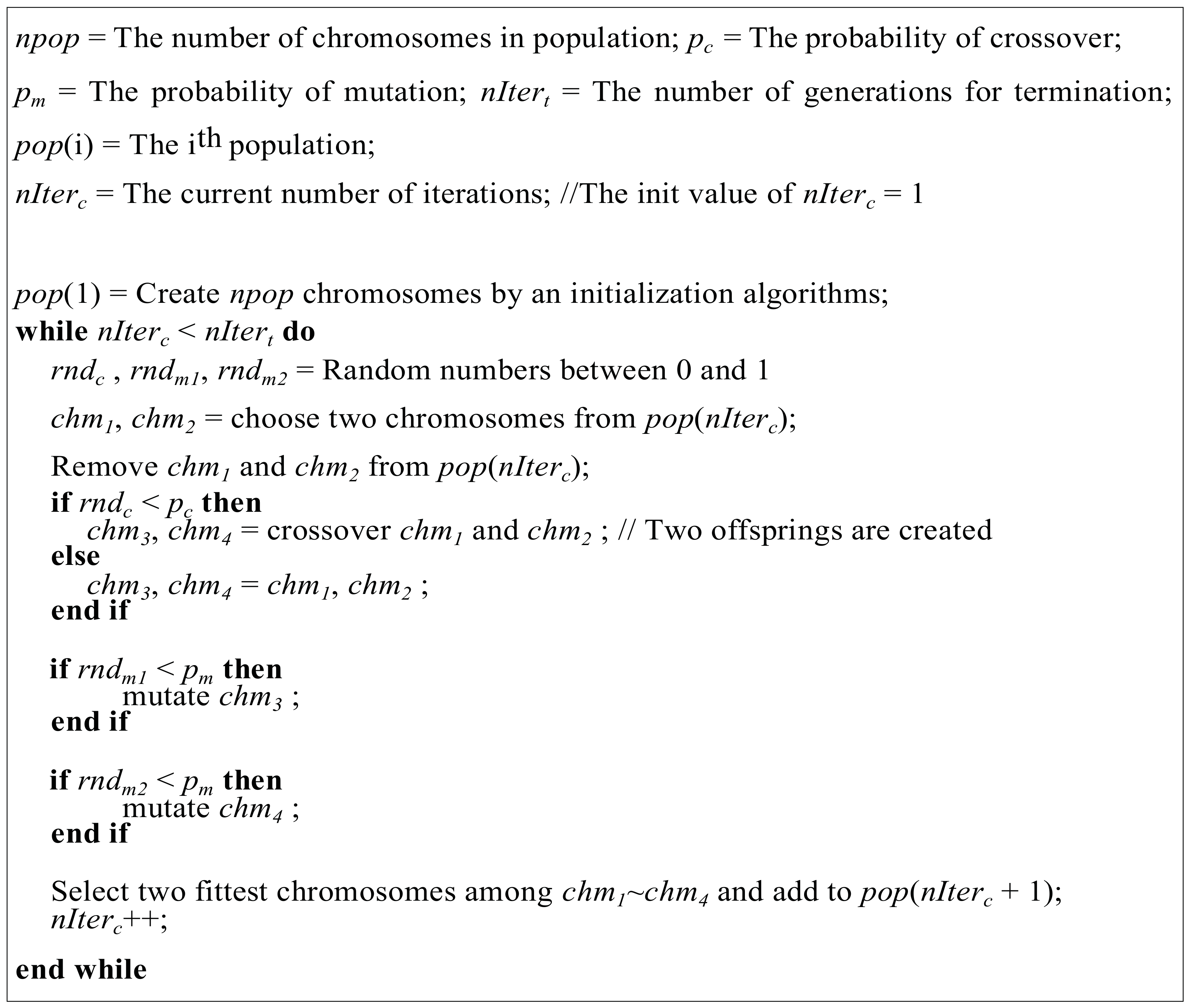
As one of most well-known global search algorithms [22,23], genetic algorithm (GA) imitates the survival and reproduction of the fittest individuals in nature. As shown in Figure 1, a typical existing GA was rewritten to be able to take a new form that is appropriate for the HSD. In this GA, there are four parameters: the number of chromosomes in the population (npop); the probability of crossover (pc), the probability of mutation (pm), and the number of iterations for termination (nIter).
A search by the GA starts from the initial population consisting of npop chromosomes created by an initialization algorithm. The search repeats nIter iterations of reproduction of the fittest individuals. In each iteration, a new population is created from the current population. To create a new population, new chromosomes are created by stochastically applying crossover and mutation to them according to pc and pm. Among two old and two new chromosomes, two fittest chromosomes are selected for the new population. After a new population has been selected, the algorithm runs repeatedly until nIterc eventually becomes smaller than nItert to find the optimized chromosome.
2.2. Metrics for Fitness Functions
Coupling, cohesion, and complexity are three commonly used structural properties to assess the quality of modules (e.g., functions, classes, and subsystems) and software systems [24,25,26,27,28]. In this study, we also use them to evaluate subsystems and define fitness functions for evaluating HSDs. Unfortunately, there is no measure that can evaluate HSDs as they are. Nonetheless, there are several complexity, cohesion, and complexity measures that can be adopted for evaluating subsystems in the existing literature. We adopt the measures and define quality measures for HSDs.
In this section, we define the notations used for describing the measures used in this paper. We then describe the complexity, cohesion, and coupling measures used for defining the fitness functions of GA.
2.2.1. Proposed Notation for HSD
Software system S consists of basic entities and dependencies between them, S = {BE, D}. BE is a set of basic entities of S. Edge d∈D represents the dependency of basic entities be1 and be2, (be1, be2)∈D through the inheritances and references between them. In Figure 2, the system has nine basic entities and dependencies between them. For example, basic entity e2 has a dependency on basic entity e1 by inheriting e1 or referencing the data or functions of e1.
The HSD of a system, S, has a hierarchical structure of {SB, R}. SB is a set of subsystems in S, including root(S) as the root of the HSD. In addition, sb in SB has a set of basic entities be(sb)⊂BE. In other words, the basic entities in be(sb) are grouped in sb, and they have grouping relationships with each other at the level of sb. In Figure 2, there are five subsystems, SB = R, S1, S2, S3, S4, and root(S) = R. Each subsystem contains several basic entities. For example, S1 and S2 have be(S1) = e3, e4, e5, e6, e7 and be(S2) = e3, e4. The basic entities in be(S1) have grouping relationships at the level of S1, and those in be(S2) have grouping relationships at the level of S2.
The relationship r∈R denotes that a subsystem is part of another subsystem called part-of relationships between subsystems. In the relationship, subsystem sb can have its parent subsystem, prt(sb)∈SB. In other words, there are part-of relationships between sb ∈SB and its children cld(sb) ⊂ SB by the edges of R between them. So, be(cld(sb)) ⊂ be(sb). In Figure 2, cld(S1) = {S2, S3}, prt(S2) = S1, and be(S2) ⊂ be(S1). Not only be(S2) ⊂ be(S1), but also S2 ⊂ R. Thus, a descendant of subsystem sb ∈ SB, dsc(sb), is part of sb. On the other hand, subsystem sb has ancestors ast(sb). For example, ast(S3) = {S1, R}.
According to part-of relationships, e∈BE belongs to one or more than one subsystem. So, basic entities can be grouped in more than one subsystem, with the part-of relationships representing the level of a subsystem wherein its basic entities have grouping relationships. For example, in Figure 2, e3 and e4 are grouped together in S2. e3 and e5 are grouped in the higher level, S1. Therefore, e3 and e4 have a more homogeneous or closer grouping relationship than that of e3 and e5.
In be(sb), there are several basic entities that do not belong to cld(sb), and the basic entities belong to sb directly, bedir(sb) ⊂ be(sb). In Figure 2, bedir(R) = {e1, e2}.
2.2.2. Complexity
A complex subsystem makes it hard for a developer to understand the subsystem. A subsystem consists of basic entities and its child subsystems; one should understand them to understand the subsystem. If there are too many constituents, the subsystem might be hard to understand. As shown in Equation (1), the complexity of a given subsystem sb, Cpx(sb), is defined by the number of its constituents, which is one of the most frequently used concepts of complexity measures [24,25].
The larger the value of Cpx(sb), the more basic entities and child subsystems there are. So, a high value of Cpx(sb) has a negative effect on an HSD.
The complexity of a given HSD, S, is computed by taking the maximum value among the complexity values of all subsystems, as presented in Equation (2).
If the complexity of an HSD is too high, there is at least a very large subsystem. Likewise, the HSD should be restructured by breaking down large subsystems or moving some of its basic entities and child subsystems to proper locations.
2.2.3. Cohesion
A subsystem needs to consist of a cohesive set of basic entities. To measure the cohesiveness, we use a similarity measure that is used in hierarchical clustering [5,29,30]. The similarities between basic entities are measured by the similarities of their feature vectors. The features of a vector for a basic entity represent other basic entities on which the basic entity has dependencies by inheritance and reference relationships. Thus, the vectors of two basic entities are similar, and they are interacting with similar basic entities. That makes them cohesive.
In this work, we use binary vectors representing whether a basic entity has dependencies of features or not. To measure the similarity between two vectors, Jaccard coefficient [5] is used. For the given basic entities be1 and be2, as shown in Equation (3), the Jaccard coefficient Jcr between them is given by:
The value of a is the sum of the features present in both. The values of b and c represent the sum of features present in just one of two vectors. The larger the value of the Jaccard coefficient, the more similar the two vectors. Thus, Jcr(be1, be2) = 0 means that there are no features represented in both vectors. In addition, when they have the same vectors, it has 1.
As provided in Equation (4), the cohesion of subsystem sb∈SB is computed by averaging the similarity between the basic entities in the boundary of the subsystem.
A large value of Coh(sb) means that the target subsystem consists of similar basic entities, and that it is cohesive.
There are two versions of cohesion for HSD S, as shown in Equations (5) and (6). The first cohesion is given by the sum of cohesion of all subsystems in S.
The second version is given by:
ρ is between 0 and 1. It can be used to give weights to cohesion values of subsystems. In our study, as presented in Equation (7), ρ is given by:
ρ makes the cohesion of a higher-level subsystem in the hierarchy more important than that in a lower level. It also has a recursive form to make the cohesion of a subsystem affected by its ancestors. So, even if a subsystem has high cohesion without ρ, the low cohesion values of its ancestors make it lose up to half of its cohesion by ρ.
2.2.4. Coupling
A subsystem of a system that is loosely coupled with other parts of the system is more manageable and understandable according to the SE principles [31]. In many previous studies [24–28], the coupling of a module is measured by counting the number of modules interacting with it. We define the coupling measure for a subsystem in a similar point of view.
The coupling of subsystem sb, Cpl(sb), is caused by the external dependencies of its basic entities on other basic entities or subsystems “outside”. In our coupling measure, the boundary of the outside of sb is defined as the boundary of prt(sb). Thus, as shown in Equation (8), the basic entities and subsystem counted as the targets of external dependencies of sb are given by:
This is to reflect the “top–down decomposition” of an HSD. A hierarchy of subsystems is built by decomposing a system into subsystems and the subsystems into sub-subsystems. Thus, a subsystem that is loosely coupled with other subsystems should be decomposed to make its offspring loosely coupled with each other, and the decomposition need not concern the coupling of the outside.
Cpl(sb) is computed by the ratio of the number of external dependencies on basic entities and subsystems in the outside of sb, ExDepbe(sb) and ExDepsb(sb), to the number of dependencies of basic entities in sb on the basic entities in prt(sb), Dep(sb), ExDepbe(sb), ExDepsb(sb), and Dep(sb) are given by Equation (9):
As provided in Equation (10), Cpl(sb) is given by:
A low value of Cpl(sb) means that sb is loosely coupled with other parts and is decomposed well in view of coupling. As shown in Equation (11), the coupling of a given HSD S is computed by aggregating the coupling values of the subsystems in S.
Cpl(S) uses the same weighting schemes used in Coh2(S). In contrast to Coh2(S), low Cpl(S) means high quality of HSD S.
In this way, a new concept of the metrics for individual metrics (i.e., complexity, cohesion, and coupling) essential for the GA that will be applied to HSD has been presented clearly by mathematically redefining them in terms of software architecture, allowing automated HSD. The actual form of utilization of such concept and corresponding notations to perform HSD is described in detail in the following section.
3. Recovering the Hierarchical Subsystem Decomposition Using GA
To achieve automated HSD recovery that is flexible to the criteria, we propose an approach to recovering HSD using GA. In Section 3.1, we describe how to represent and initialize a chromosome. In Section 3.2, we propose the GA operators (crossover and mutation) with fitness functions used in this study.
3.1. Chromosome Representation and Initialization Algorithm
We define a representation of a chromosome that encodes the characteristics of an HSD. The two most important characteristics of HSD are grouping relationships between basic entities and part-of relationships between subsystems. It is because a good subsystem is designed to have basic entities and subsystems that are homogeneous to each other and heterogeneous with the outside of the subsystem to achieve modularity [31,32].
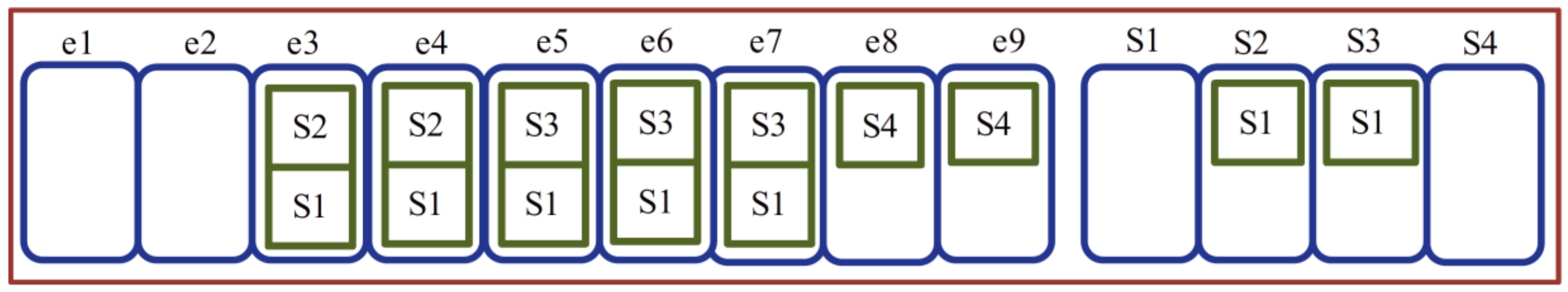
We define chromosome chr as a set of supergenes sgenes(chr), which are divided into two sets: basic entities and subsystem genes sgenesbe(chr) and sgenessb(chr) ⊂ sgenes(chr). There are a number of (|be(sb)| +(|SB|-1)) supergenes. So, a supergene has its corresponding basic entity or subsystem corrhsd(sg). Figure 3 shows an example of our chromosome representation of an HSD in Figure 2. There are (9 + (5 – 1)) supergenes for 9 basic entities and 4 subsystems except for the root of an HSD, R, in Figure 2.
Supergene sg1 ∈ igenes(sg) has a set of internal genes igenes(sg). Each ig ∈ igenes(sg) represents the supergene sg2 ∈sgenes(chr) of a subsystem where the basic entity or subsystem corrhsd(sg1) belongs. This can be denoted by corrig(sg1, sg2) = ig. Conversely, ig has a corresponding supergene sg2, which is denoted by corrsg(ig) = sg2. So, there is a subsystem sb where corrhsd(ig) = corrhsd(sg2) = sb. In igenes(sg), the internal genes are presented in “ascending” order. The first ig ∈ igenes(sg), igenes(sg,1), represents the subsystem containing corrhsd(sg) directly. The last ig ∈ igenes(sg), |igenes(sg)|), represents the subsystem containing the root of an HSD directly.
In Figure 3, supergene e5ig has two internal genes S1ig and S3ig, which have the corresponding supergenes corrsg(S1ig) = S1sg and corrsg(S1ig) = S3sg. In Figure 2, subsystems corrhsd(S1sg) = S1 and corrhsd(S3sg) = S3 contain basic entity corrhsd(e5ig) = e5. The first element of igenes(e5), igenes(sg, 1), denotes S3, which contains e5 directly; the last internal element, igenes(sg, 2), denotes S1, which belongs to the root of the given HSD in Figure 2.
We propose an initialization algorithm that aims to generate a chromosome of an HSD “arbitrarily.” The initialization algorithm consists of two phases. In the first phase, it creates subsystems having only basic entities. It is accomplished by selecting an arbitrary number of basic entities and allocating them in a new subsystem. In the second phase, part-of relationships between the subsystems are assigned until only one subsystem without its parent is left. The subsystem becomes the root of a created HSD by the initialization algorithm.
With this initial algorithm, a chromosome for HSD is generated, and the calculation through crossover and mutation will be performed to find the optimal decomposition structure with the fitness function. To achieve this, the crossover, mutation, and fitness functions have to be redefined to perform HSD. The definitions and corresponding execution processes are described in the following section.
3.2. GA Operators
3.2.1. Crossover
The method with its execution flow of crossover is proposed based on the concept and notations defined for HSD in Section 2, representing in a pseudocode form to present them clearly.
A crossover operator for HSD recovery should be able to create new chromosomes that inherit good grouping and part-of relationships of their parents. Thus, the crossover in our approach aims to remove the chromosome subsystems causing poor grouping and part-of relationships and rebuild it based on the good groupings of another chromosome.
Figure 4 presents our crossover algorithm. It consists of two sub-algorithms: selection and regrouping. First, selection is applied to two given chromosomes of a system for crossover. For each chromosome, several supergenes of subsystems are selected arbitrarily and removed to leave parts of it. Figure 5 presents the pseudocode of the selection algorithm. An example of selection for a chromosome is shown in Figure 6, and subsystem S1 is selected for removal from the HSD.
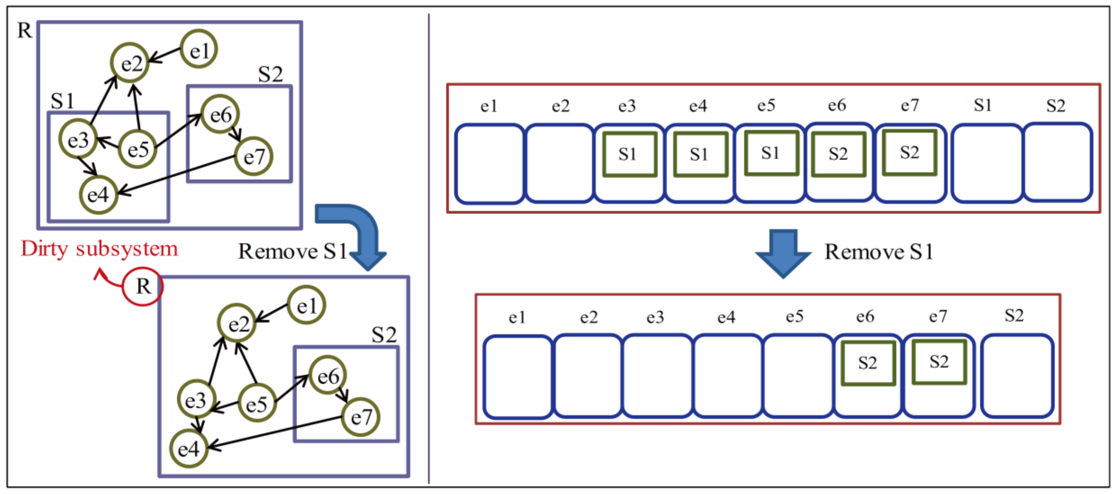
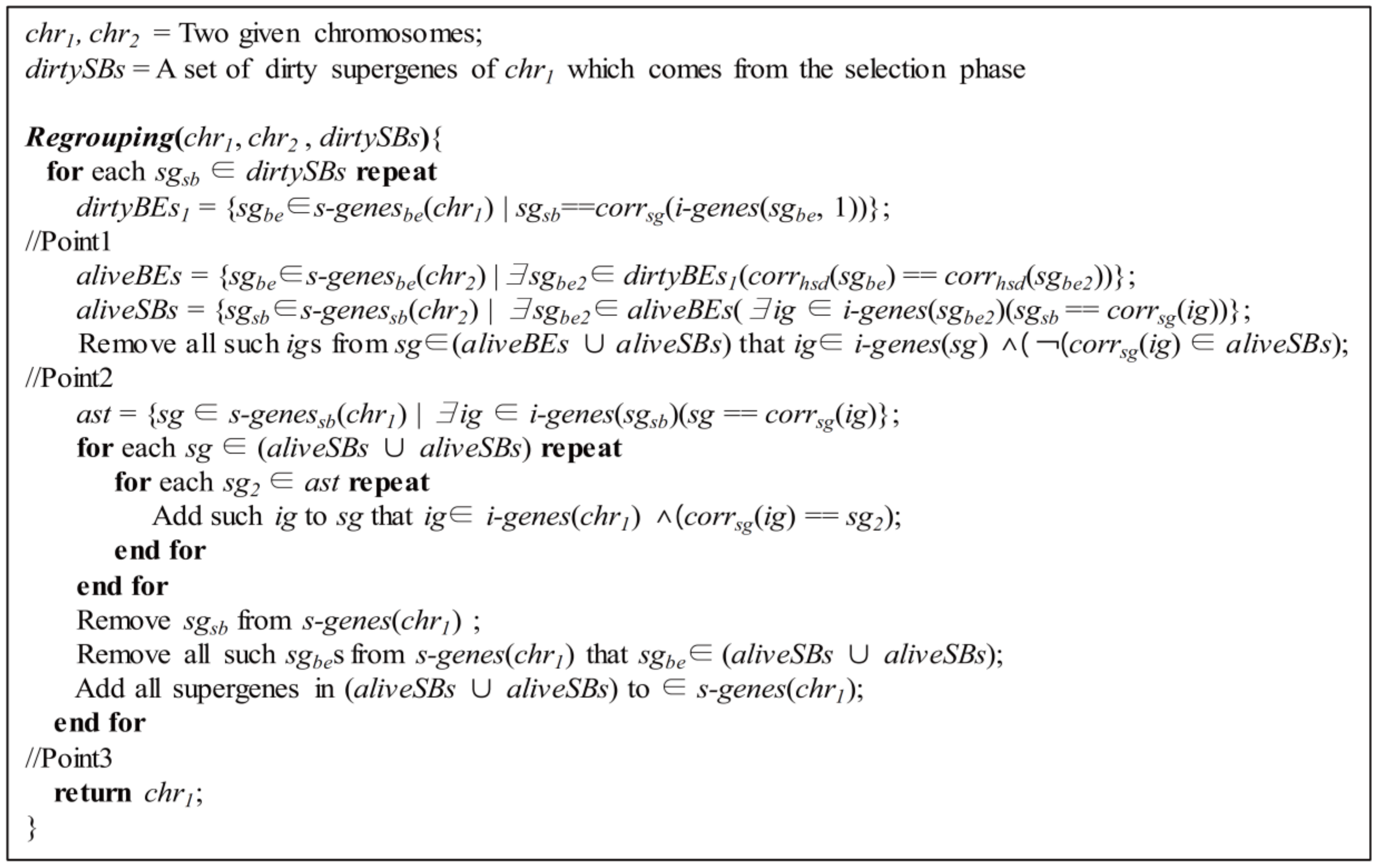
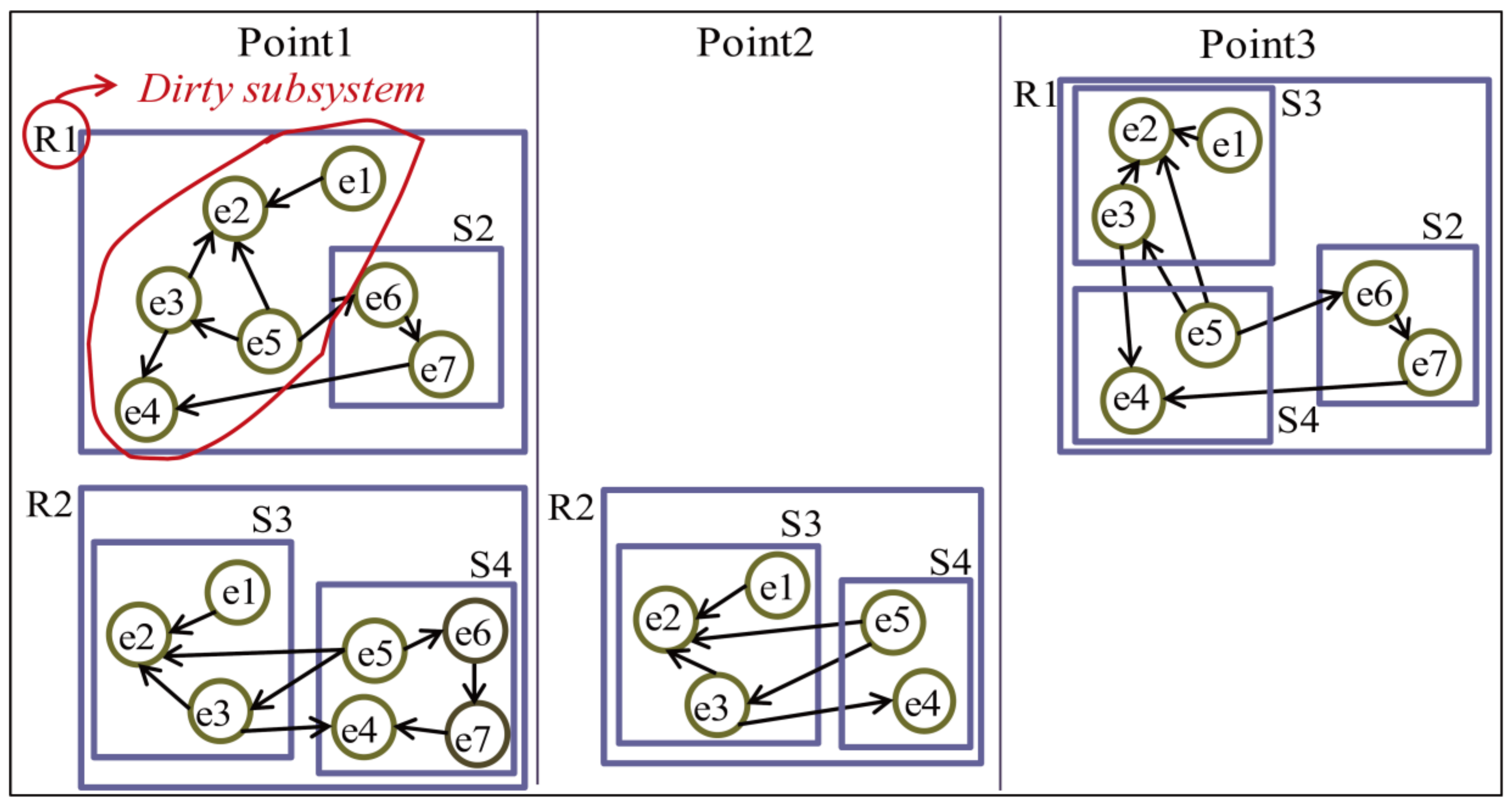
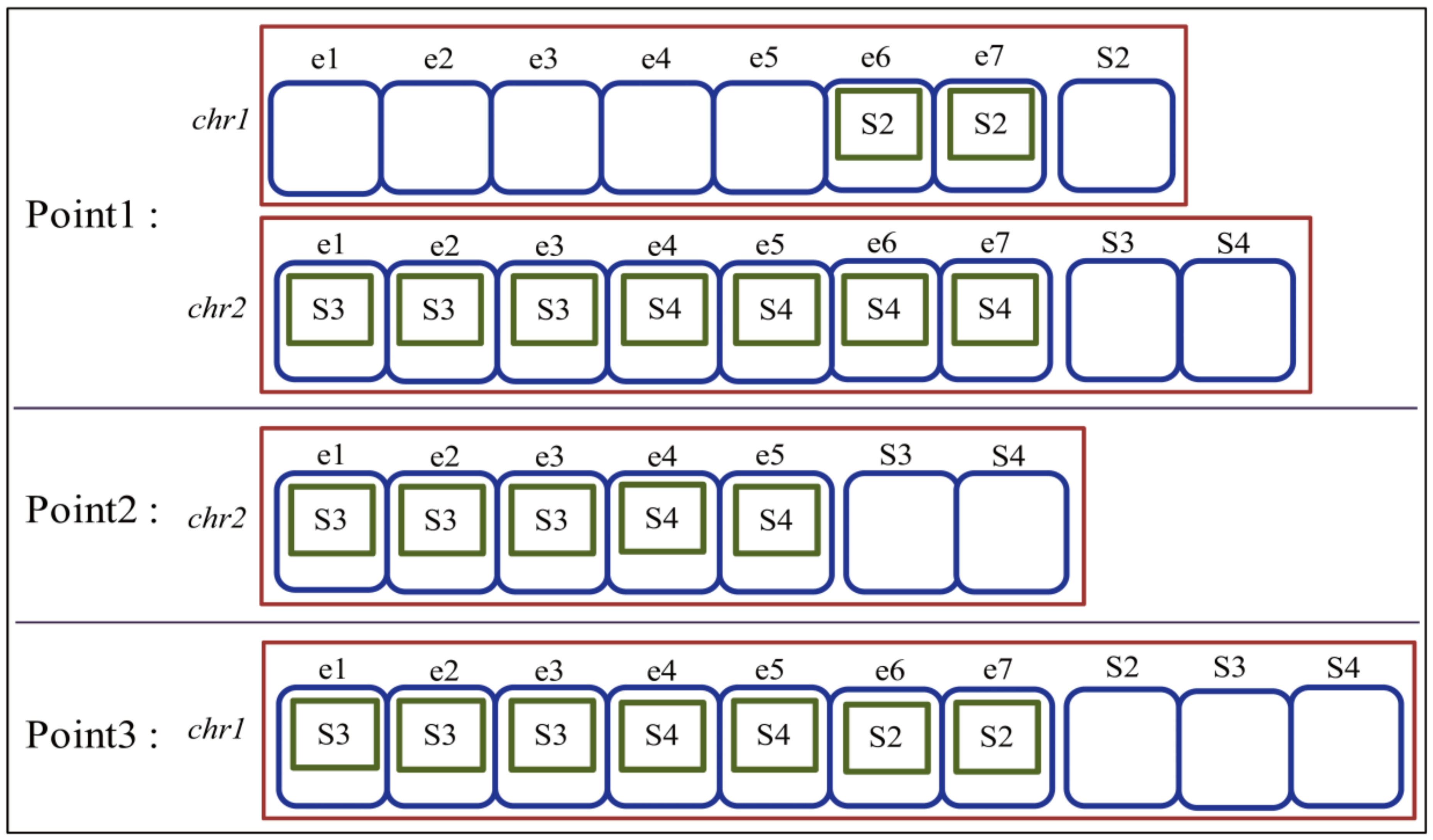
Next, regrouping regroups each chromosome’s basic entities that lose their grouping and part-of relationships based on those of the other chromosomes. After the regrouping of two given chromosomes, two new chromosomes inheriting the grouping and part-of relationships of their parents are created. Figure 7 shows the pseudocode of the grouping algorithm. Figure 8 and Figure 9 present an example of regrouping in the HSD and chromosome versions. The example shows the status of the target HSDs and chromosomes at three points of Figure 7. The first point shows the status of two given chromosomes before regrouping progresses. At point 2, part of a chromosome is created by removing the basic entities of a dirty subsystem. In addition, point 3 shows the result of regrouping after replacing the basic entities of a dirty subsystem of a chromosome with part of the other chromosome created at point 2.
3.2.2. Mutation
The method with its execution flow of mutation is proposed based on the concept and notations defined for HSD in Section 2, which is represented in a figure to present them clearly.
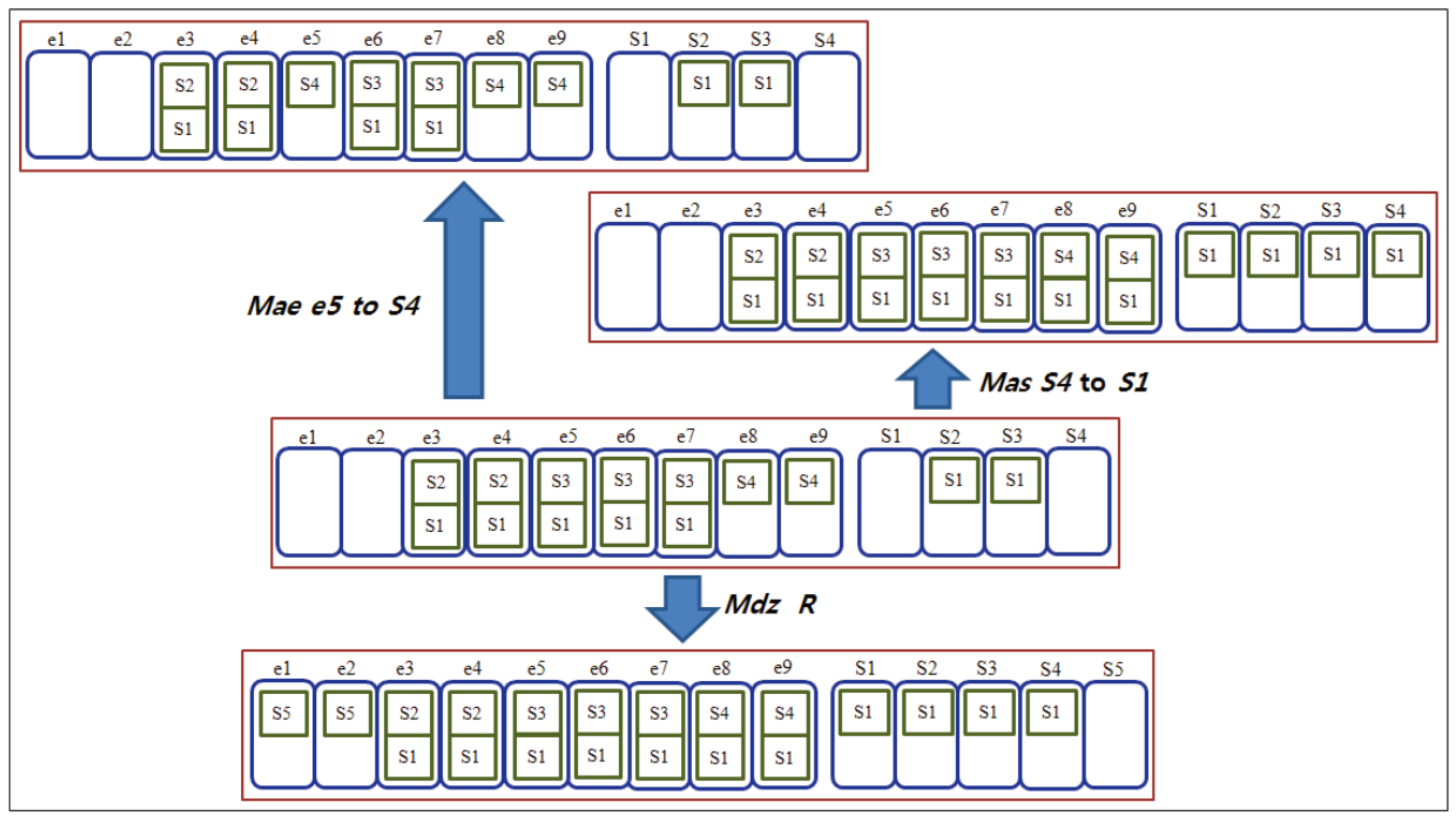
We define three mutation operators that cause small change to HSDs: (1) moving an entity (Mae), (2) moving a subsystem (Mas), and (3) modularizing (Mdz). The Mae mutation operator moves basic entities from one subsystem into another subsystem. The Mas mutation operator moves a subsystem into another subsystem. The Mdz mutation operator creates a new child of a subsystem by grouping basic entities belonging to the subsystem directly. Figure 10 shows examples of the mutation operators.
When a mutation operator is applied to an HSD during search by the GA in our approach, an operator is selected stochastically based on the number of feasible cases.
3.2.3. Fitness Function
The fitness function is proposed by using the notations for cohesion and coupling for HSD introduced in Section 2.
We define two fitness functions for experimental purposes: FF1 and FF2. They are on the structural properties, and their metrics are introduced in Section 2.2. The first fitness function, FF1, is given by Equation (12):
The higher FF1 is, the higher the quality of a given HSD. We use FF1, which is designed to produce HSDs having similar structures with dendrograms produced by hierarchical clustering algorithms for architecture recovery [5,8]. According to the formula of Coh1, FF1 is high when an HSD has many subsystems that are highly cohesive. Since a subsystem has a small number of basic entities, it commonly becomes highly cohesive.
As shown in Equation (13), FF2 is the aggregation of three structural properties: complexity, cohesion, and coupling.
This fitness function is designed to search HSDs with low complexity, high cohesion, and low coupling. A high value of FF2 means that HSD has high quality. The weight variables w1, w2, and w3 can be used to emphasize some properties among them or balance them. The change of weight values would change the objectives of a search. Therefore, a recovered HSD would have different structural characteristics according to the weight values.
If complexity is emphasized more than the others, the size of a subsystem would be reduced by decreasing the number of its basic entities by moving some basic entities to other subsystems or creating new subsystems consisting of such. If there are too many offspring in a subsystem, the offspring would also be reduced.
More weight on cohesion would lead to a rich hierarchy, similar to an HSD by FF1. Unlike Coh1 of FF1, Coh2 with ρ gives more weight to higher-level subsystems of a hierarchy. That makes FF2 with more weight on cohesion prefer wide hierarchies than deep ones because the Coh2 of low-level subsystems is highly likely to be reduced by ρ.
If coupling is emphasized, an HSD would have a relatively small number of subsystems. This is because a large subsystem can encapsulate a large number of interactions between basic entities. On the other hand, the number of offspring of a subsystem is reduced because a large number of offspring can cause a large number of interactions between them as well as high coupling. Cpl with ρ prefers deep hierarchies for the same reason as the Coh2 mentioned above.
4. Evaluation
In this section, we evaluate our approach to show how well it performs in finding an HSD intended by the given criteria with limited cost. First, we introduce our tool, HireGA (Hierarchical subsystem decomposition recovery by GA), which implements our approach. Then, we present the overview of the evaluation process, and the result of evaluation is finally described.
4.1. HireGA Tool
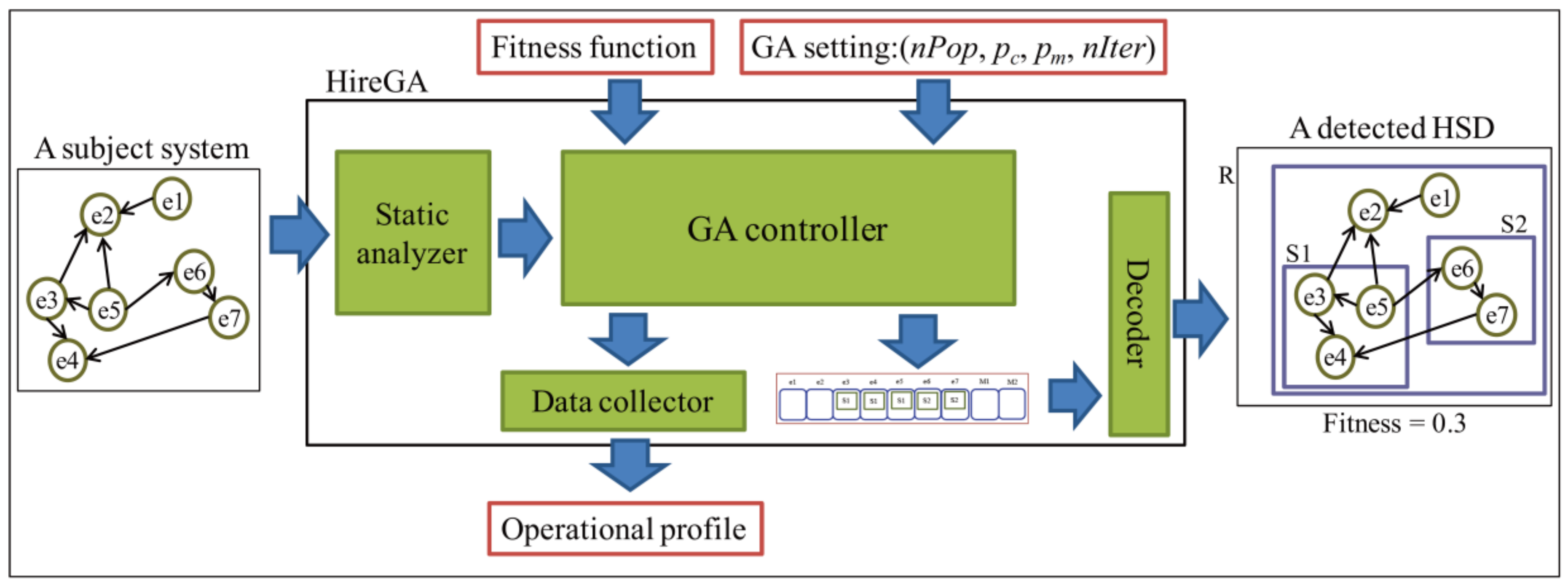
HireGA supports our approach to recovering HSDs of a system written in Java. Figure 11 depicts the overview of HireGA. The tool takes the source code of a subject system and a configuration as input. The configuration consists of fitness function and parameters related to a GA setting. The parameters consist of npop, pc, pm, and nIter, which are introduced in Section 2.1.
HireGA consists of four parts: static analyzer, GA controller, data collector, and decoder. The static analyzer conducts static analysis on the source code to figure out the basic entities and dependencies among them. The GA controller creates the initial population based on the results of analysis by the static analyzer and explores the search space in order to find an optimal HSD. The decoder decodes the chromosome detected by the GA controller into an HSD. The given fitness function evaluates chromosomes (i.e., HSDs) during the search. The data collector outputs an operational profile on crossover and mutation describing how much and how frequently they give improvement to chromosomes. The profile consists of two kinds of data: success rates and improvement degrees. They are given by Equations (14) and (15):
4.2. Overview of the Evaluation Process
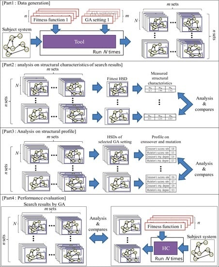
In Figure 12, we present the overview of our evaluation process, which consists of 4 parts: data generation, analysis of the structural characteristics of search results, analysis of operational profile, and performance evaluation.
In the data generation part, we replicate N times HSD recoveries for a subject system and a configuration. The two subsystems used in this evaluation, JMSN and DNSJava, are presented in Table 1 together with the number of basic entities and their description. For each subject system, we use 98 configurations, 7 fitness functions, and 14 GA settings, as presented in Table 2 and Table 3. As a result, N detected HSDs, and their operational profiles are produced for each subsystem and configuration. The fitness functions in Table 2 have different objectives from each other. For example, fitness functions 5, 6, and 7 in Table 2 target loosely coupled subsystems; the others, fitness functions 1, 2, 3, and 4, target highly cohesive ones. In this experiment, we run HireGA on a limited cost. We regard the number of fitness computations as the cost of a search because the computations take the most time in a search. As shown in Table 3, the limitation is achieved by keeping nPop · nIter = 10,000 for all GA settings.
In part 2, we evaluate the ability of our approach to detect an HSD that reflects the objectives of a given fitness function. If our approach has such ability, it will detect HSDs having different structural characteristics led by different fitness functions. We analyze and compare the structural characteristics of the detected HSDs for each subject system and its 7 fitness functions in part 1. As the target configuration of analysis, the best-performing GA setting is selected for each fitness function among the 14 settings in Table 3. The performance of searches using a given configuration is determined by the average fitness values of N detected HSDs for the configuration. The N detected HSDs for the selected 7 configurations are analyzed by the 12 analysis metrics in Table 4. The first 5 metrics are structural metrics that show the structure of a given HSD, such as the number of subsystems. The remaining 7 metrics are quality metrics that show the complexity, cohesion, and coupling of a given HSD in various ways.
In part 3, the crossover operator in our approach is evaluated. The crossover operator is the most significant operator contributing to the performance of a GA. Thus, the efficiency of crossover in search is important to guarantee the performance of our approach. To evaluate our crossover operator, we analyze operational profiles to figure out the contribution of our crossover and mutation operators to the search ability of our approach. We select 7 configurations for a subject system: 7 fitness functions in Table 2 and a GA setting for each fitness function. For the 7 configurations, we analyze the operational profiles collected in part 1. This analysis would also give clues to decide which values for a GA setting, nPop, pc, pm, and nIter, are more suitable for our approach.
In part 4, we evaluate the search ability of our approach by comparing it with that of an approach using a Hill-Climbing algorithm (HC) implemented by our mutation operators. For each fitness function in Table 2, we produce N detected HSDs by the HC. Then, the search results are compared with the search results obtained by our approach in part 1. If our GA has better performance than the HC, we can conclude that the search concept of a GA, i.e., exploring population by crossover and mutation, is more efficient than an HC’s search concept of exploring from random solution(s) only with mutation.
4.3. Analysis Results on the Structural Characteristics
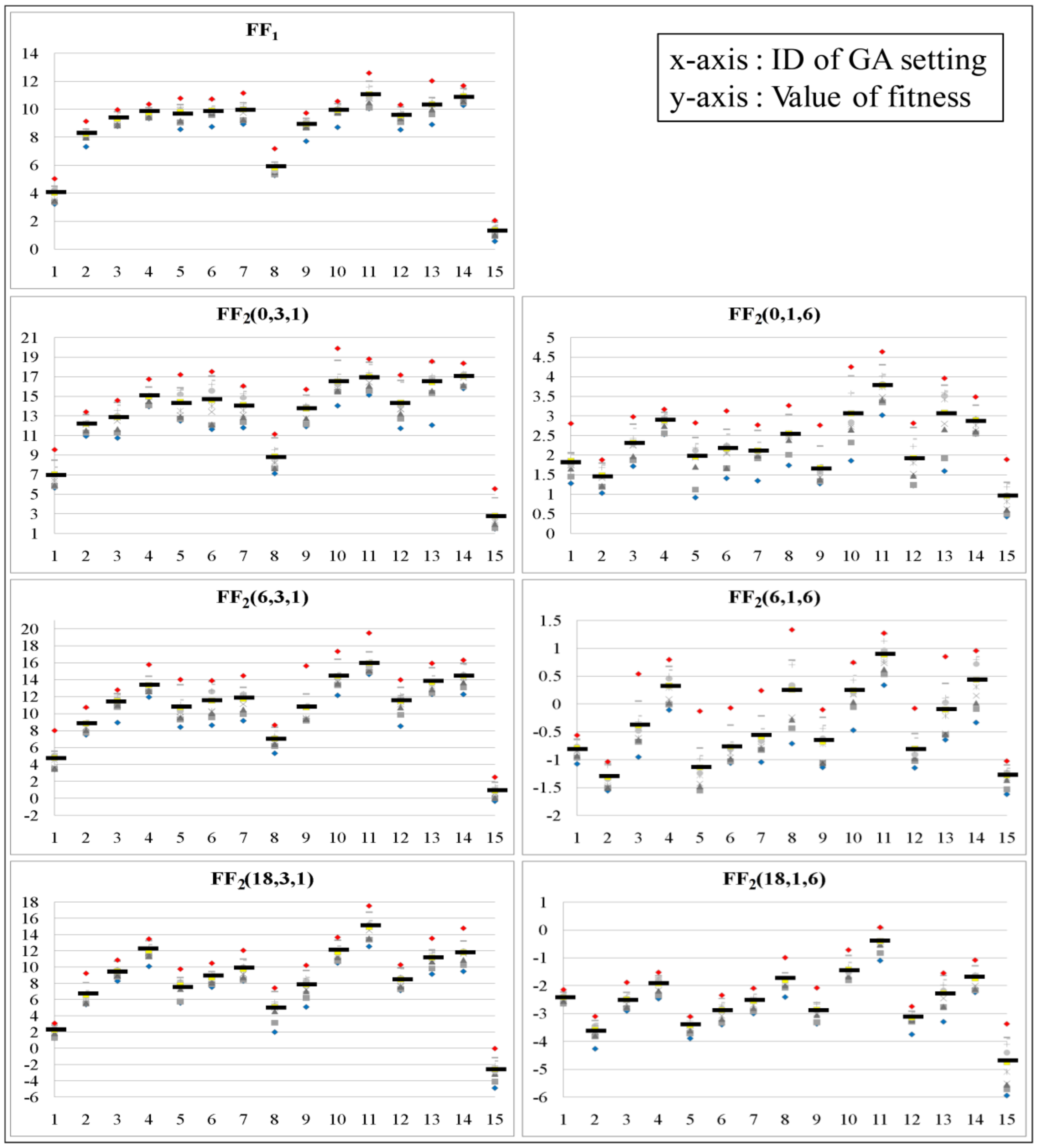
The results of searches for the fitness functions in Table 2 are shown in Figure 13 and Figure 14. In Figure 13 and Figure 14, 1 to 14 of the x-axis represent the IDs of the GA settings in Table 3. In addition, point 15 of the x-axis represents the ID of an HC. The y-axis represents the fitness values measured by fitness functions denoted on the top of each chart. The average of fitness values for each GA setting is indicated by a horizontal bar. The GA settings that give the highest average fitness for each fitness function are presented in Table 5 and Table 6. For the GA settings, the measured values of analysis metrics in Table 4 are presented in Table 7 and Table 8 for JMSN and in Table 9 and Table 10 for DNSJava.
The GAs in Table 5 and Table 6 are grouped into three in order to analyze the influence of changes of fitness functions on the structural characteristics of the detected HSDs. A change in the fitness function used means a change in the objectives of a search. The grouping allows us to fix some objectives and analyze the influence of the changes of other objectives. The three groups are as follows: GAs having different cohesion and coupling (GA1, GA3, GA6), GAs having different complexity with high cohesion (GA2, GA3, GA4), and GAs having different complexity with low coupling (GA5, GA6, GA7).
4.3.1. GAs Having Different Cohesion and Coupling
In Table 5 and Table 6, GA1 uses only the cohesion measure as fitness function FF1. GA3 and GA6 use fitness function FF2, which aggregates complexity, cohesion, and coupling. Cohesion is more emphasized in GA3, and coupling is more emphasized in GA6. So, the degree of emphasizing coupling increases from setting GA1 to GA6.
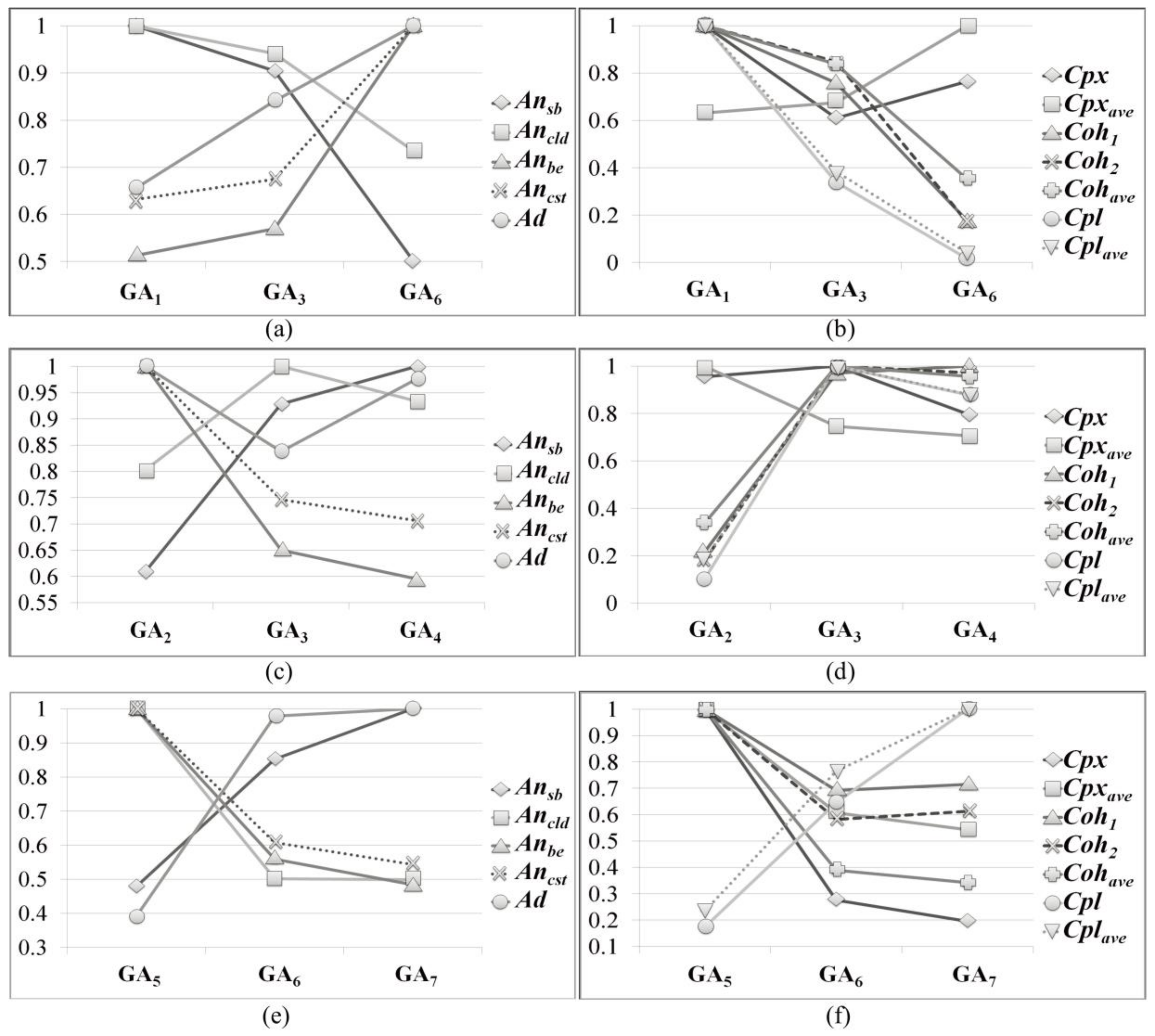
The three values of each analysis metric for GA1, GA3, and GA6 are normalized by the largest value among the three values. For example, in Figure 15b, the max value of Cpx is 0.3 of GA1, and the normalized value of Cpx of GA6 is (0.229/0.3) ≈ 0.763. The normalized values for GA1, GA3, and GA6 are presented in Figure 15a,b. This way of normalization is consistently used throughout our evaluation.
In Figure 15a, the HSDs by GA1 have relatively wide and rich hierarchies. As the coupling is emphasized, the number of subsystems and their offspring decreases. Such change coincides with the characteristics of fitness functions described in Section 3.2.3.
In Figure 15b, most of the cohesion metrics decrease, and most of the coupling metrics increase through GA1 to GA6. This coincides with the change of their fitness functions. GA2 has the lowest Cpx because complexity and cohesion are emphasized together. Cpxave tends toward high values, which is probably due to the increase in the number of basic entities belonging to a subsystem directly by emphasizing coupling. The increase overwhelms the decrease of the number of offspring, and that causes the increase of Ancst and Cpxave.
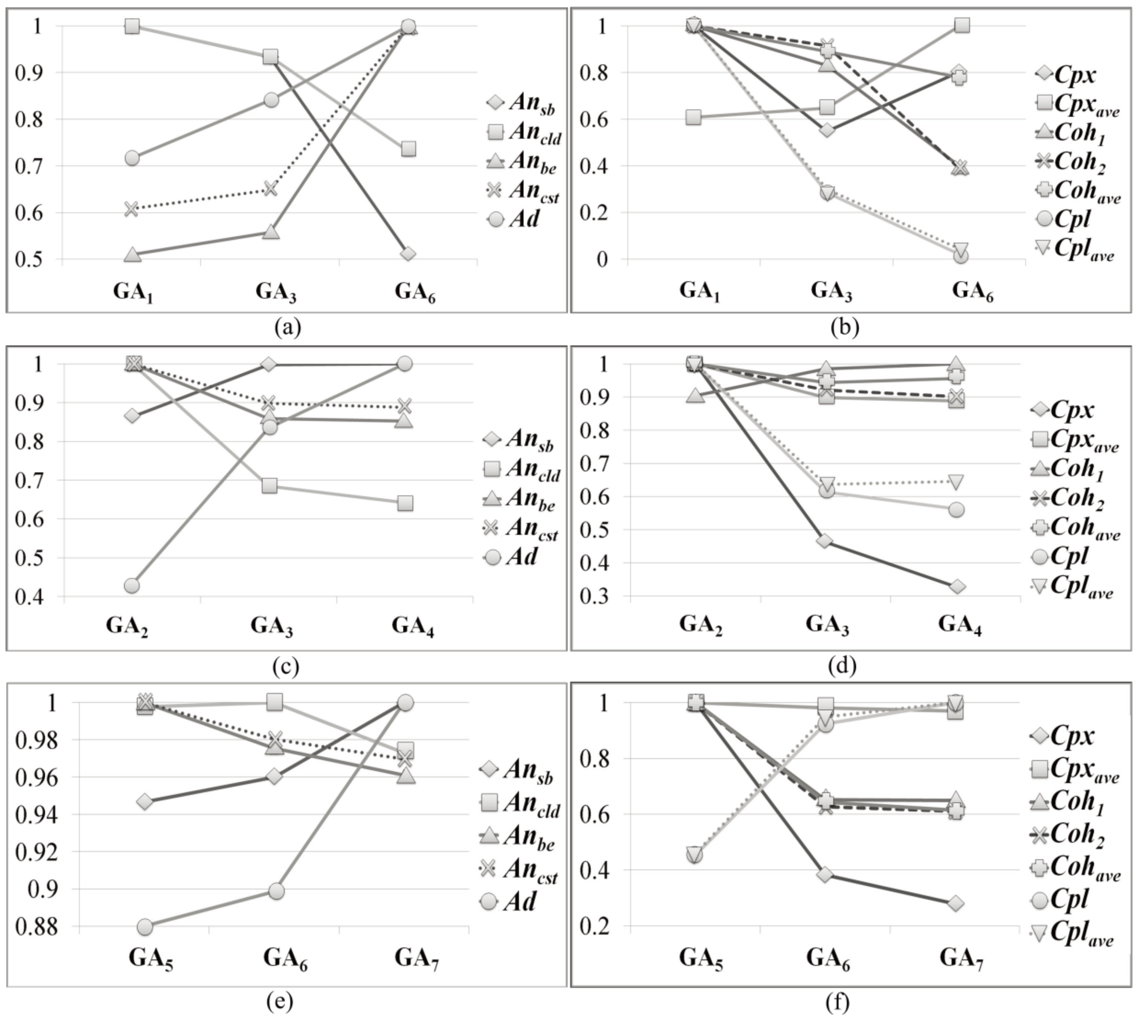
The analysis on DNSJava shows a very similar result to the result of JMSN. The measured structural and quality metrics of GA1, GA3, and GA6 for DNSJava are presented in Figure 16a,b.
4.3.2. GAs Having Different Complexity with High Cohesion
The measured structural and quality metrics of GA2, GA3, and GA4 for JMSN are presented in Figure 15c,d.
In Figure 15c, HSDs with more subsystems are detected as complexity is weighted. As w1 increases from 0 to 2, cohesion also increases by sacrificing complexity a bit in Figure 15d. Using complexity as part of a fitness function helps detect more cohesive HSDs than the ones detected by GA2. According to the definition of complexity, it forces the GA to explore HSDs with relatively rich subsystems having a small number of basic entities. So, the number of subsystems increases by making wide hierarchies. Such change can increase cohesion according to Section 3.2.3. On the other hand, coupling increases for the same reason.
When w1 increases from 2 to 6, the deep hierarchies become more preferable. A large number of offspring in subsystems cause high complexity and high coupling. Thus, the number of offspring is reduced by making deep hierarchies, and this in turn lowers not only complexity but also coupling and cohesion. The change coincides with the characteristics of fitness functions and the change of fitness functions.
The measured structural and quality metrics of GA2, GA3, and GA4 for DNSJava are presented in Figure 16c,d. According to Figure 16c, the decrease of complexity is accomplished by making the detected HSDs deep and rich. The number of offspring decreases by making deep hierarchy, and that can cause a decrease of coupling and cohesion as mentioned above.
4.3.3. GAs Having Different Complexity with Low Coupling
The measured structural and quality metrics of GA5, GA6, and GA7 for JMSN are presented in Figure 15e,f. Since coupling is emphasized, search without weight on complexity detects the HSDs having a relatively small number of subsystems. More weight on complexity, w1 = 2, makes the number of subsystems grow and the size of the subsystems shrink. Such causes high coupling according to the definition of Cpl. If coupling and cohesion are considered together, HSDs having subsystems with low coupling would be created instead of subsystems with high cohesion. So, complexity is decreased by not only increasing the number of subsystems but also making the hierarchy deeper to increase coupling as minimally as possible, but at the expense of cohesion. As a result, both cohesion and coupling deteriorate.
In the change of w1 from 2 to 6, complexity is decreased by increasing the number of subsystems in the detected HSDs. Unlike the change of w1 from 1 to 2, the depth and width of the hierarchies show little change. The increase in the number of subsystems causes an increase of coupling and cohesion. Nonetheless, cohesion shows little change because the cohesion values of the subsystems might be very low by emphasizing coupling.
The measured structural and quality metrics of GA5, GA6, and GA7 for DNSJava are presented in Figure 16e,f. The analysis on DNSJava shows very similar results to the result of JMSN, but the change of analysis metrics for DNSJava is less drastic. In our manual inspection of the resulting HSDs of GA5, they commonly have a large subsystem contributing to coupling. So, the increase of w1 decreases Cpx a lot by reducing the number of basic entities in the large subsystems. Such causes relatively small changes to the rest of the HSDs and the analysis metrics.
As we have shown in the analyses on structural characteristics for JMSN and DNSJava, the search results are varied according to fitness functions. Therefore, we can conclude that our approach can reflect different objectives of the fitness functions and produce HSDs that reflect the difference of objectives.
4.4. Analysis Results on the Operational Profile of Mutation and Crossover
As shown in Figure 13 and Figure 14, nPop = 50 and nIter = 200 always show better performance than nPop = 100 and nIter = 100, respectively. In most of the cases, the GA settings of pc = 0.5 and pm = 1.0 give the best performance. The performance of a GA is heavily dependent on its crossover and mutation operators. Likewise, the efficiencies of crossover and mutation contributing to finding a quality HSD affect the best-performing GA setting and vice versa. Therefore, in this analysis, we figure out the search efficiencies of crossover and mutation by analyzing the operational profiles of the detected HSDs by several GA settings. The analysis also leads us to the best GA settings based on the analysis result.
As the targets of the analysis, we choose the GA settings of pc = 0.5 and pm = 0.5 because they give equal chances of application to crossover and mutation. We only present the details of analysis on the results of recovery by our approach for DNSJava and the GA settings having nPop = 50 and nIter = 200. That is because the analysis on JMSN or the other GA settings gives a similar result to the presented analysis and in consideration of space.
4.4.1. Analysis on nPop and nIter
The average success rates for 10 runs with the fitness function in Table 2 are shown in Table 11. We divide a running of GA in 3 phases by dividing 200 iterations into 3 and record the success rates of crossover and mutation for each phase separately. The numbers on the top of Table 11 represent the IDs of the fitness functions in Table 2. In Figure 17a, we present charts of the normalized values of data in Table 11. In addition, Table 12 and Figure 17b show how much the fitness values are improved by applying operators.
In these charts, the success rates and improvement degrees of crossover are relatively high in phase 1 but decrease sharply through phases 2 and 3 for all cases. The mutation rates also decrease, but relatively gradually compared with crossover. Therefore, crossover plays the role of improving the quality of HSDs in the early phase of search. On the other hand, mutation plays the role of rendering relatively small changes during search.
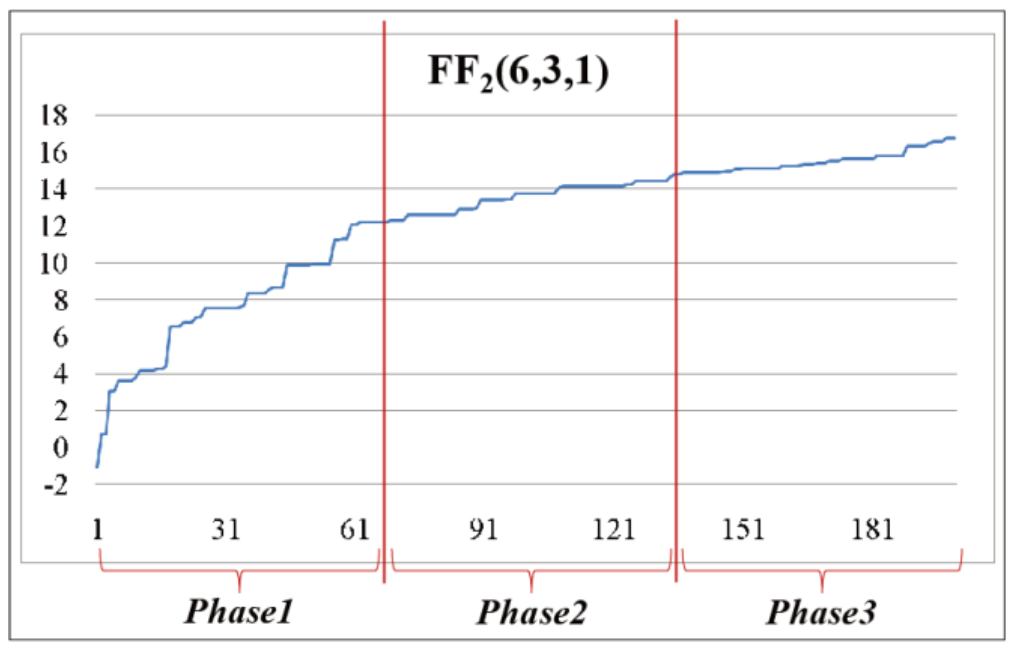
Regardless of nPop = 50 or 100, the limited number of genetic traits in the population is “consumed” by crossover, and new chromosomes with “good” traits and high quality are created rapidly in the early phase of search as shown in Figure 18, which depicts the change of fitness of the fittest HSD of each iteration. After the early phase, the fitness increases relatively slowly, and mutation contributes to the increase with higher efficiency than crossover. Thus, if the limit of cost is not expanded, it is better to increase the chances of mutation improving the chromosomes by creating new good traits. In other words, a larger number of iterations show better performance.
4.4.2. Analysis on pc and pm
In the analysis in Section 4.4.1, the efficiency of crossover is considerably reduced in the early phase of search. In the GA of Figure 1, mutation is applied after crossover is applied or skipped. Thus, the mutation could be affected by the low efficiency of a GA in the late phase of search.
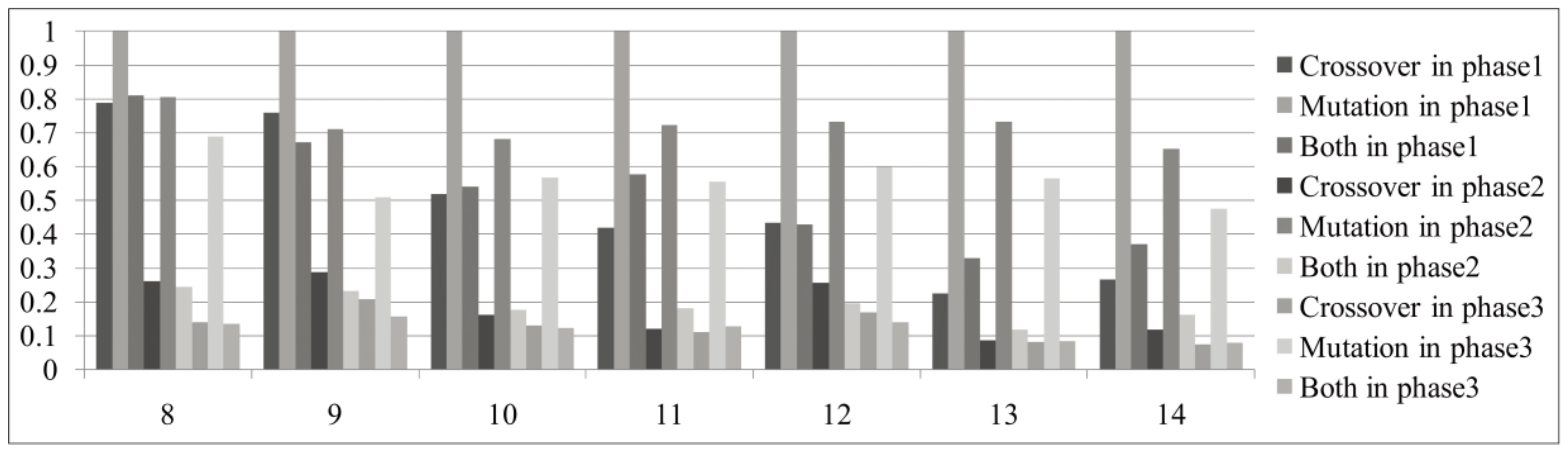
Table 13 presents the success rates of combinations of operators for GAs whose setting is nPop = 50, pc = 0.5, pm = 0.5, and nIter = 200 for the fitness functions in Table 2. There are three combinations: crossover-only, mutation-only, and both. Crossover-only occurs when crossover is applied to an HSD but mutation is skipped. Mutation-only is the opposite. The combination “both” is a case wherein crossover and mutation are applied to an HSD. The normalized values of the data in Table 13 are drawn as a chart in Figure 19.
In Figure 19, the success rates applying both crossover and mutation decrease drastically as the search proceeds, along with those of crossover-only, but mutation-only maintains relatively high success rates. We can conclude that applying mutation after applying crossover is inefficient in the late phase of search because of the low success rate of crossover. Nonetheless, applying both crossover and mutation and crossover-only is relatively efficient in the early phase. In the analysis in Section 4.4.1, the efficiency of crossover is also relatively high in the early phase. So, it is important to set pc properly to balance its efficiency in the early phase and its inefficiency in the late phase of search.
In the same perspective, mutation can also offset the improvement by crossover with poor operation. Still, it can be easily inferred that the effect of failure of mutation is far smaller than the improvement degree by crossover in the early phase based on Figure 17b. In the late phase of search, mutation plays a refining role, as analyzed in Section 4.4.1. Therefore, it is better to keep pm high during search.
The values that we used for pc and pm are (0.0, 0.5, 1.0) and (0.1, 0.5, 1.0). Among the settings, 0.5 for pc and 1.0 for pm are the most suitable values according to our analysis.
4.5. Performance Evaluation by Comparing Our Approach with Search by HC
An HC starts its search from a point of a search space and terminates when it reaches the (local) optimal solution or a given termination condition is met. To compare with our GA fairly, the HC used in this evaluation is implemented by the mutation operators of our approach to exploring neighbors. Likewise, the number of evaluations of HSDs by fitness functions is given as a termination condition for the HC. The HC is (re)started at random positions when one run of the HC is terminated before the termination condition is met. We maintain nPop • nIter = 10,000 throughout all the GA settings. This restricts the cost for a run to 10,100 evaluations at most, 10,000 for a search, and 100 for initializing a population of 100 chromosomes. When the number of evaluations by the HC reaches 10,100 during the search, the search is finished. Then, the fittest HSD is taken as an optimal solution among the detected HSDs by multiple runs of the HC.
We apply the HC to JMSN and DNSJava with the fitness functions in Table 2. The search results for the systems are presented in Figure 13 and Figure 14 together with the search results of our GA. The 15th datum in each chart represents a search result by the HC.
The performance of the HC in DNSJava is much worse than that in JMSN. As the size of a target system grows, the number of neighbors of an HSD also grows. So, the larger a system is, the higher the cost incurred by the HC to find a fitter HSD among neighbors than a given one. Such reduces the search space that can be covered by the HC at a given cost. In addition, the impact of change to an HSD by mutation in a large system is weaker than that in a small system. Therefore, the efficiency of mutation becomes lower as the size of a system grows, whereas the efficiency of our crossover becomes relatively higher.
During our experiment, we realized that HC cannot finish just one run of an HC in DNSJava. This means that an HC starts from only one point in the search space and searches as “deep” as possible. In contrast to this search strategy, an HC can (re)start multiple points to search “widely” but relatively “shallowly.” Therefore, the higher performance of GA than HC is likely caused by poor search strategy as well as the efficiency of crossover.
Thus, we take the strategy with various numbers of restarts and run the HC with them. We choose seven numbers for restarts: 1, 2, 5, 18, 20, 50, and 100. Figure 20 presets the search results of GAs in Table 3. The data of 15 to 21 represent HCs with the seven restart numbers, as presented in Table 14. Among the results of the HC with the fitness functions in Table 2, we present only the result of FF2 (6, 1, 6) because it shows relatively high or similar performance among all results and relatively high efficiency of mutation during our evaluation.
Despite the changes of the restart number for the HC, the GA in our approach always shows better performance than the HC. We conclude that the search strategy of a GA is more adequate for recovering HSDs than HCs. Our crossover operator also contributes to the outcome. Especially, as a software system for recovery expands, HC is expected to require much more resources (i.e., time) to perform similarly to GA.
The architecture of an extensive software system can be often interpreted by employing a technique Hierarchical Subsystem Decomposition (HSD), but as it is possible that the contents obtained from such a task have not been managed properly, they would not reflect the current picture. Constant update or revision can cause many changes in the software so that recovering or regenerating HSD contents is not an easy task.
This paper proposes an approach that can work through the past contents and reproduce an optimal solution that suits the design criteria well. As the objectives of such a task can be domain/system-specific or depend on the environmental conditions, the proposed approach focuses on complying with each objective effectively by utilizing a genetic algorithm creating a fitness function to work through all across search areas to deliver an optimal HSD form. The approach was subjected to the tests for evaluation where two open-source software systems having a set of 14 fitness functions in the algorithm. The architectural characteristics of the HSD types recovered by using the proposed approach varied depending on the objective given, and the result showed that the crossover type was more effective during the early search stage and the mutation enhanced the performance a little throughout the entire search process. The performance of the genetic algorithm used for the approach was analyzed in comparison with the Hill-Climbing algorithm and produced a better result in quality-wise even considering that it was in the early stage of development. The same result was expected for the proposed approach when compared with other existing approaches.
5. Related Work
5.1. Recovery Approaches for Subsystem Decomposition
There have been several studies published regarding the recovery of subsystem decomposition from the design or source code of a system.
Mitchell et al. [33] proposed a famous bunch tool for architecture recovery. The bunch tool transforms a system into a directed Module Dependency Graph (MDG) consisting of nodes representing basic entities and edges representing dependencies between entities. In addition, it decomposes MDG into several MDG partitions using a hill-climbing or simulated annealing algorithm. The bunch tool uses Modularization Quality (MQ) as a fitness function that represents the balance between the internal and external edges of MDG partitions. The MDG partitions present a flat subsystem decomposition that consists of disjoint partitions of basic entities and no part-of relationships between its subsystems.
Seng et al. [34] proposed an approach to improving subsystem decomposition. They adopted the grouping genetic algorithm (GGA) [35], which is a specialized genetic algorithm designed to solve a grouping problem with GA. They used the aggregation of five structural metrics as a fitness function: cohesion, coupling, complexity, cycles, and bottlenecks. GGA searches only the flat subsystem decomposition that fits the given fitness function. An issue with this approach, and other existing approaches, is that they cannot provide the advantages of hierarchy, which is useful for understanding a system, especially when it is large and complex [8].
Jeet et al. [36] proposed an approach that is based on a combination of a nature-inspired black-hole algorithm and a genetic algorithm, which is named the Genetic Black Hole Algorithm (GBH). The combination of evolutionary algorithms tested on various software systems and resulted in better solutions.
The studies detailed in [5,29,30] adopted hierarchical clustering algorithms, which apply a greedy strategy to cluster similar basic entities. They used hierarchical clustering algorithms to produce a dendrogram presenting similarities among basic entities. Dendrograms can be used to recover the hierarchical structure diagrams HSDs by clustering basic entities in various levels of similarity.
The authors in [9,10] proposed recovering subsystem decompositions using concept analysis. Concept analysis represents several attributes of basic entities, such as global variables in use and interacting basic entities, to build a concept lattice, which consists of partially ordered sets of concepts. Basic entities are clustered as subsystems at a proper level of the concept lattice. A concept lattice represents “part-of-relationships” between sets of basic entities sharing the same attributes.
The studies detailed in [5,9,10,29,30] are similar to our approach in that they can be used for recovering HSDs; however, they use technique-dependent forms of criteria to find high-quality HSDs. When there are criteria provided by an expert, the criteria should be transformed to specific forms suited to their techniques. This makes the approaches inflexible for recovering HSDs using various (different) forms of criteria, because the transformation is highly difficult to perform. This is especially true when complex criteria are given. In practice, hierarchical clustering algorithms require measures defining similarities between basic entities. Concept analysis is also needed to represent the relationships among basic entities as concepts. However, when the criteria are complex, such as the multi-modal criteria used in Seng et al.’s work [34], transforming the criteria to a similarity measure or to concepts is almost impossible to accomplish.
Although the existing studies are helpful in performing subsystem decomposition, they cannot provide the advantages of hierarchy that is crucial for understanding a system, especially when it is large and complex.
5.2. GA Approaches Based on Tree Representation in Other Domains
In Koza’s work [37], GA is used to create a LISP (List Processor: high-level programming language) expression, which for example is a minimal-length-expression used to fulfill a given task. The author represented a LISP expression as a tree structure, which is referred to as a syntax tree, and uses the tree structure as the individual for the GA instead of a chromosome, and crossover and mutation operators that are specific to the domain are provided. The crossover takes two syntax trees as parents, and a subtree from each tree is inherited by their children. Subsequently, the parents exchange their subtrees by each removing a subtree and attaching the subtree to the other parent in place of the removed one. As an example of syntax trees (i.e., expressions) of LISP:
T1: (OR (NOT D1)(ANDD0 D1))
T2: (OR (OR D1 (NOT D0))(AND (NOT D0))(NOT D1))
S1: (NOT D1)
S2: (AND (NOT D0))(NOT D1)).
T1 and T2 are given as the targets for crossover, and the subtrees (i.e., sub-expressions) in two syntax trees, S1 and S2, are selected for crossover. Crossover between T1 and T2 results in two new legal syntax trees:
T1’: (OR (AND (NOT D0))(NOT D1)(AND D0 D1))
T2’: (OR (OR D1 (NOT D0)) (NOT D1)).
In contrast, a mutation is performed to produce a small change in a syntax tree. There are three mutation operators and they are highly specific to the domain. For example, the editing operator simplifies an expression based on editing rules such as
(AND X X) → X.
A tree structure is one of several feasible forms used to represent a hierarchical structure. An HSD can be represented by a tree structure: nodes for subsystems and basic entities, and edges representing where subsystems and basic entities belong. Therefore, the GA is the easiest alternative considered for use in recovering HSDs [38]. In R. Lutz’s work [39], a complexity metric based on information theory was proposed, and a GA was applied to validate the metric without guarantee of the adaptability of the GA to the recovery of HSDs. To address this issue, crossover is adapted to resolve discrepancies between syntax trees and HSDs, and mutation operators suited to HSDs are applied [37].
However, the GA studied in [37,39] did not adapt well to the task of exploring HSDs because it does not consider the characteristics of each HSD, which should be considered to produce quality HSDs. First, the characteristics of an HSD are far different when using a syntax tree. The hierarchy of syntax trees represents the order of processing of sub-expressions. In an HSD, grouping relationships of basic entities (i.e., which entities are grouped together in which subsystem level, and part-of relationships among subsystems) are the most important characteristics. Second, in contrast with syntax trees, there are dependencies between the nodes of tree structures in HSDs. A node representing a basic entity should appear in a tree at least once, but only once. This means that there should be nodes representing all basic entities and that the grouping relationships between basic entities should be unique. Therefore, in the crossover for syntax trees, attaching a sub-tree to another syntax tree is equivalent to adding a sub-expression to an expression, and the result of the attachment is considered to be a legal expression. However, applying crossover to HSDs can produce illegal HSDs, which have duplicate and/or missing nodes representing basic entities. The gap between the GA and the characteristics of the HSD recovery problem requires a repair procedure after crossover [38].
The inconsistency between the GA proposed in [37,39] and the characteristics of the problem (recovering HSDs) causes a serious issue in that the actual effect of the crossover performed on HSDs is highly difficult to grasp [38]. This makes it challenging to apply the GA to HSD recovery in various circumstances. For example, when a very large-scale system requires architecture recovery, scalability can be a problem. In this case, other information, such as the change history of the system, can be used to reduce the search space by reducing the arbitrary elements in the GA and by guiding the operators to proceed in an indicated and more efficient search. In some cases, the system expert can modify several elements of GA, such as the initialization of the algorithm, and crossover and mutation operations, to fit them to a specific problem. Therefore, to apply GA in various circumstances, the GA should be developed by analyzing the characteristics of the HSD, and these characteristics should be reflected to the elements of the GA. This was one of the primary reasons why we began this study, which was to develop such a GA.
6. Threats to Validity
(Implementation of a GA) In several studies, various approaches to implement a GA are proposed [11,34,39,40]. Among all feasible implementations, we selected one of the simplest implementations (provided by [11]) to avoid distortions associated with using a more complex and advanced GA.
(Weights of FF2) During our experiment, we used more values for the weight variables of FF2 than we presented in the evaluation. Although we did not present the analysis on all weights because of space considerations, the conclusions for the omitted weights were the same as those reached in the analysis presented.
(Decrease of crossover efficiency in the late stages of a search) The decrease in efficiency results from two causes: a small population size or the inherent convergence problem of GAs [11]. The former can be resolved by increasing the population size, but this increases the cost of a search. Regarding the convergence problem, several techniques have been proposed to resolve it. For example, a GA can use a selection strategy to compose a new generation during the search, and this new generation is one of the most influential elements toward achieving GA convergence. Our approach can adapt other selection strategies, such as roulette wheel selection [11], instead of the greedy selection strategy that we actually used in this study.
(Implementation of HC) We use the simplest implementation of HC, the first-ascent HC, which moves the search to the first discovered neighbor with higher quality [40] for the same reason that we use a simple implementation of a GA. There could be other implementations of HC that provide higher performance in recovering an HSD. If there is such an implementation, it would be worth using, because HC is simpler to understand and implement than GA. A study on various implementations of an HC algorithm for HSD recovery is one of our planned future studies.
7. Conclusions
In this paper, we have proposed an approach to recovering an HSD, which provided an architecture-level understanding of a software system. A method of understanding the software system at the architecture level was provided in this study along with an HSD scheme useful for reducing the possibility of software erosions. When an HSD of a software system is recovered, the objectives of recovery are given by experts. The objectives of recovery may be domain-specific or system-specific. They may also vary according to the purpose and circumstances of recovery. Thus, an approach to recovering an HSD of a software system should be able to adopt various objectives of recovery. To achieve this, we have proposed a recovery approach using GA, which is able to adopt various objectives easily as a fitness function and find a quality HSD in a vast search space.
To apply a GA in our approach, we provided a chromosome representation that represents grouping relationships among basic entities and part-of relationships among subsystems as the characteristics of an HSD affecting its quality. The initialization algorithm was designed to create arbitrary HSDs for initializing the population of a GA. Crossover was proposed to create new HSDs inheriting the grouping and part-of relationships from existing HSDs in the population. Mutation operators were provided to create a new HSD by rendering a small change to the grouping and the part-of relationships of an HSD in the population. In addition, fitness functions were designed to have different objectives, which were presented by the structural properties of an HSD and metrics assessing the properties.
In our evaluation, we evaluated the ability of our approach to recover different HSDs according to different objectives of recovery. We applied our approach to two open source software systems with fitness functions having different objectives of recovery. Then, we analyzed the search result to figure out whether our approach could find different HSDs according to the various fitness functions. As a result, our approach recovered HSDs having different structural characteristics intended by the fitness functions and their objectives of recovery.
Afterward, we evaluated how much our crossover operator contributed to the search efficiency of our approach, since crossover is a key feature significantly influencing the performance of a GA. We analyzed the contributions of our crossover and mutation operators to the search efficiency of the GA. We also compared our approach with an approach using an HC. As a result, crossover provided great efficiency to a search by contributing to the early-phase search, whereas mutation played the role of refinement throughout the entire search. On the other hand, the comparison of our approach and an approach using an HC showed us that the GA was the better strategy for the recovery. According to the analysis and comparison, our crossover operator had a significant role during the search. The performance of our GA was attributed to the efficiency of our crossover operator.
Our approach can be applied to recover an HSD intended by various objectives given as fitness functions. The change history or design specification of a system could be used for the establishment of the objectives of recovery by experts. For example, the change history of a software system could be used for establishing an objective to recover an HSD with low change impact among subsystems. In different objectives, our approach may show different behavior and require different calibration. Therefore, we plan to repeat the evaluation of our approach in various objectives.
Author Contributions
Conceptualization, J.H. and Y.-S.S.; Data curation, J.-H.H., J.H. and Y.-S.S.; Formal analysis, J.H.; Funding acquisition, J.-H.H. and Y.-S.S.; Investigation, Y.-S.S.; Methodology, J.-H.H., J.H. and Y.-S.S.; Project administration, Y.-S.S.; Resources, J.H.; Software, J.H.; Supervision, Y.-S.S.; Validation, J.-H.H., J.H. and Y.-S.S.; Visualization, J.-H.H. and J.H.; Writing—original draft, J.-H.H., J.H. and Y.-S.S.; Writing—review and editing, J.-H.H., J.H. and Y.-S.S. All authors have read and agreed to the published version of the manuscript.
Funding
This work was supported by the National Research Foundation of Korea (NRF) grant funded by the Korea government (MSIT) (No. NRF-2017R1C1B5018295). In addition, this research was supported by Energy Cloud R&D Program through the National Research Foundation of Korea (NRF) funded by the Ministry of Science, ICT (NRF-2019M3F2A1073385).
Acknowledgments
The part of this paper [41] was presented at The 11th International Conference on Computer Science and its Applications (CSA 2019) Dec 18–20, 2019, University of Macau, People’s Republic of China. An early version of this paper was presented at CSA 2019, proposing a basic idea of using a genetic algorithm for hierarchical system decomposition (HSD) briefly and evaluating the performance of idea from a single perspective in terms of complexity, cohesion, and coupling measures. By contrast, this paper presents a specific notation for utilizing the genetic algorithm for HSD along with the concrete concepts for those three aspects followed by a new proposal for the crossover and mutation methods, which are considered to be the key to genetic algorithms, within the framework of HSD. In addition, for the performance evaluation, an additional target system was used in the experiment for verification compared to the conference proceeding paper in which only one target system was used. Further, the reliability of the verification method was enhanced by describing the changing process of fitness functions and quality metrics in detail. Meanwhile, the level of completeness and quality of the paper has been largely increased by supplementing the related study section and analyzing possible threats to validity.
Conflicts of Interest
The authors declare no conflict of interest.
Abbreviations
| HSD | Hierarchical Subsystem Decomposition |
| GA | genetic algorithm |
| HC | Hill-Climbing algorithm |
| FSC | Future Sustainability Computing |
References
- Gharbi, M.; Koschel, A.; Rausch, A. Software Architecture Fundamentals: A Study Guide for the Certified Professional for Software Architecture—Foundation Level iSAQB Compliant; Rocky Nook: San Rafael, CA, USA, 2019; pp. 20–131. [Google Scholar]
- Cervantes, H.; Kazman, R. Designing Software Architectures: A Practical Approach, 1st ed.; Addison-Wesley Professional: Boston, MA, USA, 2016; pp. 1–41. [Google Scholar]
- Bass, L.; Clements, P.; Kazman, R. Software Architecture in Practice, 3rd ed.; Addison-Wesley Professional: Boston, MA, USA, 2012; pp. 3–60. [Google Scholar]
- Faitelson, D.; Heinrich, R.; Tyszberowicz, S. Functional Decomposition for Software Architecture Evolution. In Proceedings of the 5th International Conference on Model-Driven Engineering and Software Development CCIS, Porto, Portugal, 19–21 February 2017; Volume 880, pp. 377–400. [Google Scholar]
- Maqbool, O.; Babri, H. Hierarchical clustering for software architecture recovery. IEEE Trans. Softw. Eng. 2007, 33, 759–780. [Google Scholar] [CrossRef]
- Lee, K.S.; Hong, B.W.; Kim, Y.; Ahn, J.; Lee, C.G. Split-Jaccard Distance of Hierarchical Decompositions for Software Architecture. IEICE Trans. Inf. Syst. 2015, E98-D, 712–716. [Google Scholar] [CrossRef] [Green Version]
- Chhabra, J.K. Improving modular structure of software system using structural and lexical dependency. Inf. Softw. Technol. 2017, 82, 96–120. [Google Scholar] [CrossRef]
- Andreopoulos, B.; An, A.; Tzerpos, V.; Wang, X. Clustering large software systems at multiple layers. Inf. Softw. Technol. 2007, 49, 244–254. [Google Scholar] [CrossRef] [Green Version]
- Kim, H.; Bae, D.-H. Object-oriented concept analysis for software modularization. IET Softw. 2008, 2, 134–148. [Google Scholar] [CrossRef]
- Lindig, C.; Snelting, G. Assessing modular structure of legacy code based on mathematical concept analysis. In Proceedings of the 19th International Conference on Software Engineering, Boston, MA, USA, 17–23 May 1997; pp. 349–359. [Google Scholar]
- Reeves, C.R.; Rowe, J.E. Genetic Algorithms: Principles and Perspectives: A Guide to GA Theory; Springer Science+Business Media: New York, NY, USA, 2013. [Google Scholar]
- Harman, M.; Mansouri, A. Search Based Software Engineering: Introduction to the Special Issue of the IEEE Transactions on Software Engineering. IEEE Trans. Softw. Eng. 2010, 36, 737–741. [Google Scholar] [CrossRef]
- Ghrabat, M.J.J.; Ma, G.; Maolood, I.Y.; Alresheedi, S.S.; Abduljabbar, Z.A. An effective image retrieval based on optimized genetic algorithm utilized a novel SVM-based convolutional neural network classifier. Hum. Cent. Comput. Inf. Sci. (HCIS) 2019, 9, 1–29. [Google Scholar] [CrossRef]
- Zhang, F.; Wu, T.; Pan, J.; Ding, G.; Li, Z. Human motion recognition based on SVM in VR art media interaction environment. Hum. Cent. Comput. Inf. Sci. (HCIS) 2019, 9, 1–15. [Google Scholar] [CrossRef]
- Bhatnagar, A.; Gambhir, V.; Thakur, M.K. A New Perspective to Stable Marriage Problem in Profit Maximization of Matrimonial Websites. J. Inf. Process. Syst. JIPS 2018, 14, 961–979. [Google Scholar]
- Hai, X.; Zhao, C. Optimization of Train Working Plan based on Multiobjective Bi-level Programming Model. J. Inf. Process. Syst. JIPS 2018, 14, 487–498. [Google Scholar]
- Haladuick, S.; Dann, M.R. Genetic Algorithm for Inspection and Maintenance Planning of Deteriorating Structural Systems: Application to Pressure Vessels. Infrastructures 2018, 3, 32. [Google Scholar] [CrossRef] [Green Version]
- Duan, K.; Fong, S.; Siu, S.W.I.; Song, W.; Guan, S.S.-U. Adaptive Incremental Genetic Algorithm for Task Scheduling in Cloud Environments. Symmetry 2018, 10, 168. [Google Scholar] [CrossRef] [Green Version]
- Wang, Z.-J.; Zhan, Z.-H.; Zhang, J. Solving the Energy Efficient Coverage Problem in Wireless Sensor Networks: A Distributed Genetic Algorithm Approach with Hierarchical Fitness Evaluation. Energies 2018, 11, 3526. [Google Scholar] [CrossRef] [Green Version]
- Huh, J.-H. Server operation and virtualization to save energy and cost in future sustainable computing. Sustainability 2018, 10, 1919. [Google Scholar] [CrossRef] [Green Version]
- Huh, J.-H.; Seo, Y.-S. Understanding Edge Computing: Engineering Evolution with Artificial Intelligence. IEEE Access 2019, 7, 164229–164245. [Google Scholar] [CrossRef]
- Banzhaf, W.; Nordin, P.; Keller, R.E.; Francone, F.D. Genetic Programming: An Introduction; Morgan Kaufmann: Burlington, MA, USA, 1997; pp. 23–67. [Google Scholar]
- Buontempo, F. Genetic Algorithms and Machine Learning for Programmers: Create AI Models and Evolve Solutions; Pragmatic Bookshelf: Raleigh, NC, USA, 2019; pp. 6–12. [Google Scholar]
- Chidamber, S.; Kemerer, C. A metrics suite for object oriented design. IEEE Trans. Softw. Eng. 1994, 20, 476–493. [Google Scholar] [CrossRef] [Green Version]
- Bansiya, J.; Davis, C. A hierarchical model for object-oriented design quality assessment. IEEE Trans. Softw. Eng. 2002, 28, 4–17. [Google Scholar] [CrossRef]
- Sarkar, S.; Rama, G.M.; Kak, A.C. Api-based and information-theoretic metrics for measuring the quality of software modularization. IEEE Trans. Softw. Eng. 2007, 33, 14–32. [Google Scholar] [CrossRef] [Green Version]
- Sarkar, S.; Kak, A.C.; Rama, G.M. Metrics for measuring the quality of modularization of large-scale object-oriented software. IEEE Trans. Softw. Eng. 2008, 34, 700–720. [Google Scholar] [CrossRef]
- Harrison, R.; Counsell, S.; Nithi, R. An evaluation of the MOOD set of object-oriented software metrics. IEEE Trans. Softw. Eng. 1998, 24, 491–496. [Google Scholar] [CrossRef] [Green Version]
- Andritsos, P.; Tzerpos, V. Information-theoretic software clustering. IEEE Trans. Softw. Eng. 2005, 31, 150–165. [Google Scholar] [CrossRef]
- Lung, C.H.; Zaman, M.; Nandi, A. Applications of clustering techniques to software partitioning, recovery and restructuring. J. Syst. Softw. 2004, 73, 227–244. [Google Scholar] [CrossRef]
- Sommerville, I. Software Engineering, 10th ed.; Pearson: London, UK, 2015; pp. 15–42. [Google Scholar]
- Ghezzi, C.; Jazayeri, M.; Mandrioli, D. Fundamentals of Software Engineering, 2nd ed.; Prentice Hall: Upper Saddle River, NJ, USA, 2015; pp. 45–58. [Google Scholar]
- Mitchell, B.S.; Mancoridis, S. On the automatic modularization of software systems using the Bunch tool. IEEE Trans. Softw. Eng. 2006, 32, 193–208. [Google Scholar] [CrossRef] [Green Version]
- Seng, O.; Bauer, M.; Biehl, M.; Pache, G. Search-based improvement of subsystem decompositions. In Proceedings of the 7th Annual Conference on Genetic and evolutionary computation, Washington, DC, USA, 25–29 June 2005; pp. 1045–1051. [Google Scholar]
- Mutingi, M.; Mbohwa, C. Grouping Genetic Algorithms: Advances and Applications; Springer: Cham, Switzerland, 2016; pp. 45–65. [Google Scholar]
- Jeet, K.; Dhir, R. Software Architecture Recovery using Genetic Black Hole Algorithm. ACM Sigsoft Softw. Eng. Notes 2015, 40, 1–5. [Google Scholar] [CrossRef]
- Koza, J.R. Genetic Programming: On the Programming of Computers by Means of Natural Selection; The MIT Press: Cambridge, MA, USA, 1992; pp. 63–79. [Google Scholar]
- Räihä, O. A survey on search-based software design. Comput. Sci. Rev. 2010, 4, 203–249. [Google Scholar] [CrossRef] [Green Version]
- Lutz, R. Evolving good hierarchical decompositions of complex systems. J. Syst. Archit. 2001, 47, 613–634. [Google Scholar] [CrossRef]
- O’Keeffe, M.; Cinnéide, M. Search-based refactoring: An empirical study. J. Softw. Maint. Evol. Res. Pract. 2008, 20, 345–364. [Google Scholar] [CrossRef]
- Seo, Y.-S.; Huh, J.-H. An Approach to Automating Structure Decomposition in Large Scale System. In Proceedings of the 11th International Conference on Computer Science and its Applications (CSA 2019), Macau, China, 18–20 December 2019; pp. 1–6. [Google Scholar]
Figure 1.
Pseudocode of the genetic algorithm (GA) used in this study.

Figure 2.
Example of Hierarchical Subsystem Decomposition (HSD).

Figure 3.
Example of a chromosome.

Figure 4.
Pseudocode of the crossover operator.

Figure 5.
Pseudocode of the selection algorithm.

Figure 6.
Example of the selection.

Figure 7.
Pseudocode of the regrouping algorithm.

Figure 8.
Example of regrouping: chromosome version.

Figure 9.
Example of regrouping: HSD version.

Figure 10.
Examples of mutation operators.

Figure 11.
Overview of HireGA.

Figure 12.
Overview of our evaluation process.

Figure 13.
Fitness values of the detected HSDs by GAs in Table 3 for JMSN.
Figure 13.
Fitness values of the detected HSDs by GAs in Table 3 for JMSN.

Figure 14.
Fitness values of the detected HSDs by GAs in Table 3 for DNSJava.
Figure 14.
Fitness values of the detected HSDs by GAs in Table 3 for DNSJava.

Figure 15.
Normalized values of analysis metrics of GAs in Table 5 for JMSN.
Figure 15.
Normalized values of analysis metrics of GAs in Table 5 for JMSN.

Figure 16.
Normalized values of analysis metrics of GAs in Table 6 for DNSJava.
Figure 16.
Normalized values of analysis metrics of GAs in Table 6 for DNSJava.


Figure 18.
Change of the highest fitness value during search in nPop = 50 and nIter = 200 for FF2 (6, 3, 1) of DNSJava.
Figure 18.
Change of the highest fitness value during search in nPop = 50 and nIter = 200 for FF2 (6, 3, 1) of DNSJava.

Figure 19.
Normalized success rates in Table 13.
Figure 19.
Normalized success rates in Table 13.

Figure 20.
Fitness values of detected HSDs of DNSJava by GAs in Table 3 and HCs with various restart numbers.
Figure 20.
Fitness values of detected HSDs of DNSJava by GAs in Table 3 and HCs with various restart numbers.


Table 1.
Subject systems used in the evaluation.
| System | # of Basic Entity | Description |
|---|---|---|
| JMSN 1.2.2 | 33 | A pure Java Microsoft MSN clone |
| DNSJava 1.5.0 | 93 | An implementation of DNS in Java |
Table 2.
Fitness functions used in the evaluation.
| ID | Target System | FF | w1 | w2 | w3 |
|---|---|---|---|---|---|
| 1 | JMSN | FF1 | - | - | - |
| 2 | JMSN | FF2 | 0 | 3 | 1 |
| 3 | JMSN | FF2 | 2 | 3 | 1 |
| 4 | JMSN | FF2 | 6 | 3 | 1 |
| 5 | JMSN | FF2 | 0 | 1 | 6 |
| 6 | JMSN | FF2 | 2 | 1 | 6 |
| 7 | JMSN | FF2 | 6 | 1 | 6 |
| 8 | DNSJava | FF1 | - | - | - |
| 9 | DNSJava | FF2 | 0 | 3 | 1 |
| 10 | DNSJava | FF2 | 6 | 3 | 1 |
| 11 | DNSJava | FF2 | 18 | 3 | 1 |
| 12 | DNSJava | FF2 | 0 | 1 | 6 |
| 13 | DNSJava | FF2 | 6 | 1 | 6 |
| 14 | DNSJava | FF2 | 18 | 1 | 6 |
Table 3.
GA settings used in the evaluation.
| ID | nPop | pc | pm | nIter |
|---|---|---|---|---|
| 1 | 100 | 0.0 | 1.0 | 100 |
| 2 | 100 | 0.5 | 0.1 | 100 |
| 3 | 100 | 0.5 | 0.5 | 100 |
| 4 | 100 | 0.5 | 1.0 | 100 |
| 5 | 100 | 0.9 | 0.1 | 100 |
| 6 | 100 | 0.9 | 0.5 | 100 |
| 7 | 100 | 0.9 | 1.0 | 100 |
| 8 | 50 | 0.0 | 1.0 | 200 |
| 9 | 50 | 0.5 | 0.1 | 200 |
| 10 | 50 | 0.5 | 0.5 | 200 |
| 11 | 50 | 0.5 | 1.0 | 200 |
| 12 | 50 | 0.9 | 0.1 | 200 |
| 13 | 50 | 0.9 | 0.5 | 200 |
| 14 | 50 | 0.9 | 1.0 | 200 |
Table 4.
Analysis metrics to analyze the structural characteristics of a detected HSD.
| Metrics | Description |
|---|---|
| Ansb | The number of subsystem in a given HSD |
| Ancld | |
| Anbe | |
| Ancst | Ancld+Anbe |
| Ad | The average depth of the leaves of S |
| Cpx | Cpx in Section 2.2 |
| Cpxave | |
| Coh1 | Coh1 in Section 2.2 |
| Coh2 | Coh2 in Section 2.2 |
| Cohave | |
| Cpl | Cpl in Section 2.2 |
| Cplave |
Table 5.
GA settings with the highest average for JMSN.
| GAID | FF(w1, w2, w3) | nPop, pc, pm, nIter |
|---|---|---|
| GA1 | FF1 | 50, 0.5, 1.0, 200 |
| GA2 | FF2(0, 3, 1) | 50, 0.9, 1.0, 200 |
| GA3 | FF2(2, 3, 1) | 50, 0.5, 1.0, 200 |
| GA4 | FF2(6, 3, 1) | 50, 0.5, 1.0, 200 |
| GA5 | FF2(0, 1, 6) | 50, 0.5, 0.5, 200 |
| GA6 | FF2(2, 1, 6) | 50, 0.5, 1.0, 200 |
| GA7 | FF2(6, 1, 6) | 50, 0.5, 1.0, 200 |
Table 6.
GA settings with the highest average for DNSJava.
| ID | FF(w1, w2, w3) | nPop, pc, pm, nIter |
|---|---|---|
| GA1 | FF1 | 50, 0.5, 1.0, 200 |
| GA2 | FF2(0, 3, 1) | 50, 0.9, 1.0, 200 |
| GA3 | FF2(6, 3, 1) | 50, 0.5, 1.0, 200 |
| GA4 | FF2(18, 3, 1) | 50, 0.5, 1.0, 200 |
| GA5 | FF2(0, 1, 6) | 50, 0.5, 1.0, 200 |
| GA6 | FF2(6, 1, 6) | 50, 0.5, 1.0, 200 |
| GA7 | FF2(18, 1, 6) | 50, 0.5, 1.0, 200 |
Table 7.
Values of structural metrics of GAs in Table 5 for JMSN.
Table 7.
Values of structural metrics of GAs in Table 5 for JMSN.
| GAID | Ansb | Ancld | Anbe | Bncst | Ad |
|---|---|---|---|---|---|
| GA1 | 19.533 | 1.934 | 1.668 | 2.622 | 2.500 |
| GA2 | 11.600 | 1.462 | 2.846 | 3.749 | 3.824 |
| GA3 | 17.667 | 1.821 | 1.850 | 2.799 | 3.204 |
| GA4 | 19.033 | 1.700 | 1.695 | 2.647 | 3.735 |
| GA5 | 5.500 | 2.834 | 5.817 | 6.830 | 1.524 |
| GA6 | 9.800 | 1.421 | 3.249 | 4.148 | 3.811 |
| GA7 | 11.500 | 1.412 | 2.813 | 3.710 | 3.895 |
Table 8.
Values of quality metrics of GAs in Table 5 for JMSN.
Table 8.
Values of quality metrics of GAs in Table 5 for JMSN.
| GAID | Cpx | Cpxave | Coh1 | Coh2 | Cohave | Cpl | Cplave |
|---|---|---|---|---|---|---|---|
| GA1 | 0.300 | 0.079 | 4.681 | 2.905 | 0.240 | 2.981 | 0.217 |
| GA2 | 0.175 | 0.114 | 0.782 | 0.437 | 0.067 | 0.100 | 0.015 |
| GA3 | 0.183 | 0.085 | 3.546 | 2.462 | 0.201 | 1.011 | 0.083 |
| GA4 | 0.145 | 0.080 | 3.653 | 2.393 | 0.192 | 0.888 | 0.073 |
| GA5 | 0.833 | 0.207 | 1.195 | 0.849 | 0.217 | 0.013 | 0.003 |
| GA6 | 0.229 | 0.126 | 0.827 | 0.494 | 0.084 | 0.048 | 0.008 |
| GA7 | 0.163 | 0.112 | 0.854 | 0.520 | 0.074 | 0.074 | 0.011 |
Table 9.
Values of structural metrics of GAs in Table 6 for DNSJava.
Table 9.
Values of structural metrics of GAs in Table 6 for DNSJava.
| GAID | Ansb | Ancld | Anbe | Bncst | Ad |
|---|---|---|---|---|---|
| GA1 | 42.3 | 1.986 | 2.162 | 3.157 | 3.683 |
| GA2 | 34.2 | 2.711 | 2.749 | 3.748 | 2.241 |
| GA3 | 39.5 | 1.855 | 2.362 | 3.367 | 4.322 |
| GA4 | 39.6 | 1.741 | 2.343 | 3.328 | 5.177 |
| GA5 | 21.3 | 1.449 | 4.348 | 5.300 | 5.038 |
| GA6 | 21.6 | 1.452 | 4.241 | 5.196 | 5.143 |
| GA7 | 22.5 | 1.413 | 4.179 | 5.139 | 5.724 |
Table 10.
Values of quality metrics of GAs in Table 6 for DNSJava.
Table 10.
Values of quality metrics of GAs in Table 6 for DNSJava.
| GAID | Cpx | Cpxave | Coh1 | Coh2 | Cohave | Cpl | Cplave |
|---|---|---|---|---|---|---|---|
| GA1 | 0.202 | 0.033 | 11.218 | 6.700 | 0.265 | 6.271 | 0.242 |
| GA2 | 0.240 | 0.040 | 8.550 | 6.657 | 0.250 | 2.908 | 0.114 |
| GA3 | 0.111 | 0.036 | 9.323 | 6.134 | 0.236 | 1.785 | 0.072 |
| GA4 | 0.078 | 0.036 | 9.461 | 5.999 | 0.239 | 1.636 | 0.074 |
| GA5 | 0.425 | 0.057 | 6.852 | 4.147 | 0.322 | 0.060 | 0.005 |
| GA6 | 0.162 | 0.056 | 4.467 | 2.600 | 0.207 | 0.123 | 0.012 |
| GA7 | 0.118 | 0.055 | 4.451 | 2.533 | 0.198 | 0.133 | 0.011 |
Table 11.
Success rates of operators in nPop = 50 and nIter = 200 for fitness functions in Table 2 of DNSJava.
Table 11.
Success rates of operators in nPop = 50 and nIter = 200 for fitness functions in Table 2 of DNSJava.
| Operators | 8 | 9 | 10 | 11 | 12 | 13 | 14 |
|---|---|---|---|---|---|---|---|
| Crossover in phase 1 | 0.301 | 0.253 | 0.220 | 0.208 | 0.118 | 0.112 | 0.137 |
| Mutation in phase 1 | 0.392 | 0.341 | 0.442 | 0.474 | 0.288 | 0.466 | 0.482 |
| Crossover in phase 2 | 0.110 | 0.106 | 0.080 | 0.063 | 0.077 | 0.046 | 0.066 |
| Mutation in phase 2 | 0.285 | 0.226 | 0.297 | 0.325 | 0.212 | 0.341 | 0.334 |
| Crossover in phase 3 | 0.062 | 0.081 | 0.062 | 0.057 | 0.052 | 0.043 | 0.041 |
| Mutation in phase 3 | 0.247 | 0.179 | 0.242 | 0.268 | 0.188 | 0.277 | 0.277 |
Table 12.
Improvement degrees of operators in nPop = 50 and nIter = 200 for fitness functions in Table 2 of DNSJava.
Table 12.
Improvement degrees of operators in nPop = 50 and nIter = 200 for fitness functions in Table 2 of DNSJava.
| Operators | 8 | 9 | 10 | 11 | 12 | 13 | 14 |
|---|---|---|---|---|---|---|---|
| Crossover in phase 1 | 0.285 | 0.424 | 0.535 | 0.864 | 0.292 | 0.422 | 0.689 |
| Mutation in phase 1 | 0.047 | 0.148 | 0.175 | 0.221 | 0.132 | 0.153 | 0.267 |
| Crossover in phase 2 | 0.154 | 0.340 | 0.278 | 0.303 | 0.116 | 0.077 | 0.147 |
| Mutation in phase 2 | 0.059 | 0.159 | 0.178 | 0.207 | 0.152 | 0.136 | 0.180 |
| Crossover in phase 3 | 0.134 | 0.312 | 0.273 | 0.292 | 0.126 | 0.093 | 0.093 |
| Mutation in phase 3 | 0.059 | 0.152 | 0.153 | 0.172 | 0.139 | 0.148 | 0.175 |
Table 13.
Success rates of the combination of operators in nPop = 50 and nIter = 200 for fitness functions in Table 2 of DNSJava.
Table 13.
Success rates of the combination of operators in nPop = 50 and nIter = 200 for fitness functions in Table 2 of DNSJava.
| Combination of Operators | 8 | 9 | 10 | 11 | 12 | 13 | 14 |
|---|---|---|---|---|---|---|---|
| Crossover in phase 1 | 0.181 | 0.151 | 0.137 | 0.122 | 0.069 | 0.061 | 0.078 |
| Mutation in phase 1 | 0.230 | 0.199 | 0.264 | 0.290 | 0.158 | 0.272 | 0.294 |
| Both in phase 1 | 0.186 | 0.134 | 0.143 | 0.167 | 0.068 | 0.089 | 0.109 |
| Crossover in phase 2 | 0.060 | 0.057 | 0.043 | 0.035 | 0.041 | 0.023 | 0.035 |
| Mutation in phase 2 | 0.185 | 0.142 | 0.180 | 0.210 | 0.116 | 0.200 | 0.192 |
| Both in phase 2 | 0.056 | 0.046 | 0.046 | 0.053 | 0.031 | 0.032 | 0.047 |
| Crossover in phase 3 | 0.032 | 0.042 | 0.034 | 0.032 | 0.027 | 0.022 | 0.022 |
| Mutation in phase 3 | 0.158 | 0.101 | 0.150 | 0.161 | 0.095 | 0.153 | 0.140 |
| Both in phase 3 | 0.031 | 0.031 | 0.033 | 0.037 | 0.022 | 0.023 | 0.024 |
Table 14.
Number of restarts in a run of Hill-Climbing algorithm (HC).
| ID | # of Restart |
|---|---|
| 15 | 1 |
| 16 | 2 |
| 17 | 5 |
| 18 | 10 |
| 19 | 20 |
| 20 | 50 |
| 21 | 100 |
© 2020 by the authors. Licensee MDPI, Basel, Switzerland. This article is an open access article distributed under the terms and conditions of the Creative Commons Attribution (CC BY) license (http://creativecommons.org/licenses/by/4.0/).
Share and Cite
MDPI and ACS Style
Huh, J.-H.; Hwa, J.; Seo, Y.-S. Hierarchical System Decomposition Using Genetic Algorithm for Future Sustainable Computing. Sustainability 2020, 12, 2177. https://doi.org/10.3390/su12062177
AMA Style
Huh J-H, Hwa J, Seo Y-S. Hierarchical System Decomposition Using Genetic Algorithm for Future Sustainable Computing. Sustainability. 2020; 12(6):2177. https://doi.org/10.3390/su12062177
Chicago/Turabian StyleHuh, Jun-Ho, Jimin Hwa, and Yeong-Seok Seo. 2020. "Hierarchical System Decomposition Using Genetic Algorithm for Future Sustainable Computing" Sustainability 12, no. 6: 2177. https://doi.org/10.3390/su12062177
Note that from the first issue of 2016, this journal uses article numbers instead of page numbers. See further details here.