Review

A Comparative Assessment of Analytical Fate and Transport Models of Organic Contaminants in Unsaturated Soils

by
Maria Grazia Stoppiello
1,
Giusy Lofrano
2,3,*,
Maurizio Carotenuto
2,
Giacomo Viccione
1,
Claudio Guarnaccia
1 and
Leonardo Cascini
1
1
Department of Civil Engineering, University of Salerno, via Giovanni Paolo II 132, 84084 Fisciano (SA), Italy
2
Department of Chemical and Biology, University of Salerno, via Giovanni Paolo II 132, 84084 Fisciano (SA), Italy
3
Centro Servizi Metrologici e Tecnologici Avanzati (CeSMA), University of Naples “Federico II”, via Cinthia ed. 7, 80126 Naples, Italy
*
Author to whom correspondence should be addressed.
Sustainability 2020, 12(7), 2949; https://doi.org/10.3390/su12072949
Submission received: 12 February 2020 / Revised: 20 March 2020 / Accepted: 3 April 2020 / Published: 7 April 2020
(This article belongs to the Special Issue Assessment of Industrial and Man-Made Hazards Due to Chemicals)

Abstract

:
Analytical models for the simulation of contaminants’ fate and transport in the unsaturated zone are used in many engineering applications concerning groundwater resource management and risk assessment. As a consequence, several scientific studies dealing with the development and application of analytical solutions have been carried out. Six models have been selected and compared based on common characteristics to identify pros and cons as well as to highlight any difference in the final output. The analyzed models have been clustered into three groups according to the assumptions on contaminant source and physico-chemical mechanisms occurring during the transport. Comparative simulations were carried out with five target contaminants (Benzene, Benzo(a)pyrene, Vinyl Chloride, Trichloroethylene and Aldrin) with different decay’s coefficient, three types of soil (sand, loam and clay) and three different thicknesses of the contaminant source. The calculated concentration at a given depth in the soil for the same contamination scenario varied greatly among the models. A significant variability of the concentrations was shown due to the variation of contaminant and soil characteristics. As a general finding, the more advanced is the model, the lower the predicted concentrations; thus, models that are too simplified could lead to outcomes of some orders of magnitude greater than the advanced one.

Graphical Abstract

1. Introduction

The release of organic contaminants into the environment represents a growing threat for groundwater and human health, as evidenced by the concentrations measured in several groundwater bodies [1,2,3,4,5]. Groundwater contamination is a significant environmental issue because it can damage potable water supply, endangering human health [6,7], and can affect aquatic ecosystems [8,9]. Organic contaminants moving in groundwater come from both point sources (solid waste tips, landfills, leaking storage tanks and leaking sewers) and diffuse sources (agricultural activities and farmyard drainage) [10]. Most of the fate and transport processes take place into the unsaturated zone [11], commonly known as vadose zone, posing a great concern in terms of environmental preservation and protection [12].
Due to the increasing interest in groundwater protection, models for simulating contaminants fate and transport in the unsaturated zone are a valuable and useful tool in many scientific and engineering applications [13,14,15,16,17]. They allow to evaluate the concentration of the chemicals at the point of exposure on the basis of source concentration [18] or they are useful in the assessment of the best technical solution in remediation practices [19,20,21,22,23].
The modelling of transport processes in the vadose zone is a challenging task [24], more complex than the modelling of fate and transport of contaminants in water bodies [25]. On one hand, a wide range of chemicals with variable physical-chemical properties can migrate through the unsaturated zone and interact between them and with soil; on the other hand, different transport mechanisms (advection; dispersion-diffusion) and reaction processes (sorption; abiotic transformation; biodegradation) can act simultaneously in two coupled phases (air and water) [26,27]. Several modelling approaches are available in the scientific literature, ranging from models that solve a single equation (solute transport) [28,29,30] to more complex models that solve a set of governing equations (e.g., groundwater flow, solute transport, heat movement, etc.) [31,32]. Models can be classified as analytical or numerical [33]. Numerical models allow simulating contaminant transport for both steady-state and transient groundwater flow, in three-dimensional, heterogeneous and anisotropic media with complex initial and boundary conditions, for multi-contaminant systems with different types of reactions. However, this high complexity requires a large number of input parameters, which may affect the reliability and accuracy of the prediction. This makes them unsuitable for many applications [34]. Analytical models are based on closed form solutions of governing equations; thus, they require a high level of simplification of the hydrogeological setting. Usually, they assume homogeneous soils, simple geometries, constant or highly simplified initial and boundary conditions and the transport of a single component [35]. Hence, they are characterized by ease of use and a limited number of input parameters. These peculiarities make them especially suitable for Tier II risk assessment [34,36].
Different reviews discussing many aspects of organic contaminant fate and transport models in unsaturated zone are presented in literature. In [37] models dealing with solute transport in heterogeneous media are discussed, by presenting their theoretical aspects and related applications. Vanclooster and co-workers [38] focus upon solute transport mechanisms at core scale and field scale and describe some modelling approaches. In [26] and [39] the authors analyze fate and transport of volatile organic compounds (VOCs), with experimental and modelling studies [39], providing a wide list of models [26]. Šimůnek [40] describes several models reproducing mechanisms of preferential and non-equilibrium flow and transport. Finally, Nolan and co-workers [41] tested seven transport models for pesticides with the data sets of two test sites.
None of the existing reviews focus exclusively on a comparison of analytical models. Furthermore, in the available reviews, analytical models are often described in qualitative terms neglecting their comparison in terms of numerical outputs. In order to fill this gap, a review of analytical models from a quantitative point of view is proposed in this paper. Pros and cons as well as differences in the outcomes of the different models are finally reported as result of this comparison. Six models have been selected among several unsaturated zone models existing in the scientific literature. They are presented in ASTM [42], Troldborg and co-workers (2009) [43] and (2008) [44], Verginelli and Baciocchi [45], Enfield and co-workers [46], Spence and Walden [47] and later discussed in Section 2. They model the fate and transport of organic contaminants dissolved in the aqueous phase from unsaturated zone to groundwater, assuming steady-state flow and constant parameters over the time. Comparative simulations have been carried out by using five target contaminants (Benzene, Benzo(a)pyrene, Vinyl Chloride, Trichloroethylene, Aldrin) widespread in contaminated sites and characterized by different physico-chemical properties (e.g., density, solubility, biodegradation rates), three types of soils (sand, loam and clay) and three different thickness L1 of the contaminant source, as discussed in Section 3.

2. Models Description

Analytical solutions of the selected models, named as I, II, III, IV, V and VI are listed in Table 1.
They share the following common features: (i) the assessment of the concentration of a single contaminant dissolved in aqueous phase that moves from a source located in the unsaturated zone to the water table; (ii) the negligible effect related to the movement of substances in the non-aqueous phase; (iii) the small number of geometrical, hydrogeological and chemical input data; (iv) the use of a set of simplifying assumptions that allows to obtain analytical solutions. These characteristics make them straightforward tools in many applications such as the analysis of groundwater vulnerability to pesticides contamination as well as the risk assessment of contaminated sites [48,49,50,51]. They differ mainly in their assumptions on the source and in the physico-chemical mechanisms as highlighted in Table 2.
The reference spatial domain assumed by the models is depicted in Figure 1. It consists of an unsaturated layer, lower bounded by an aquifer. The contaminant source, located in the upper region, is a parallelepiped shape with edges L1 (thickness), X and Y. Upper and lower positions of the source along the z-axis are given by Lf and L2, respectively, with reference to the water table and by Ld with reference to the ground surface. The unsaturated zone is characterized by fixed homogeneous and isotropic hydrogeological properties θ, θw, θa, ρb, Ksat, foc, Ieff, according to the hypotheses of the models. The physical-chemical characteristics of the contaminants are indicated by H, Da0, Dw0, S, Koc. The selected models, except Model I, consider the degradation processes of the contaminant in water phase using a first-order kinetic formulation, where λ is the degradation constant.
The total concentration of the contaminant is expressed by Equation (1):
C tot = M tot ρ b   V ,
whereas the concentration of the contaminant in the different phases (water; solid and air) is expressed by Equation (2):
C w = M w θ w V
The mass of the contaminant sorbed by the soil fraction upon the mass of the affected soil Cs and the mass of contaminant in vapor phase upon the volume of pore air Ca are given by Equations (3) and (4), respectively:
C s = M s ρ b   V ,
C a = M a θ a V .
In all models, the partitioning of the chemicals among these three different phases is expressed by instantaneous linear equilibrium.
When low solute concentration occurs, a linear adsorption isotherm can be assumed [52]. Thus, the ratio between Cs and Cw is constant and equal to Kd:
C s = K d · C w ,
where
K d = f oc · K oc
The liquid-vapor partition is evaluated through Henry’s Law:
C a = H · C w
On the basis of Equation (7), the dissolved concentration in pore water Cw can be evaluated from Ctot:
C w = K SW · C tot
where Ksw is expressed by Equation (9)
K SW = ρ b θ W + ρ b K d + H θ a ,
representing the dissolution of soil contaminants into infiltrating rainwater, according to the hypothesis of instantaneous and linear equilibrium.
The maximum value of Cw is the solubility (S) of the contaminant. Therefore, taking into account air, water and solid phases, the maximum Ctot is
C tot ; sat = S K SW .
Some of the selected models (Models III, IV, VI; Table 1) take into account the presence of a residual NAPL (Non-Aqueous Phase Liquid) in the source. This allows to consider an initial Ctot higher than Ctot;sat. For these models, when the measured Ctot is higher than Ctot;sat it is possible to consider Ctot as a sum of two components:
C tot = C tot ; sat + C NAPL
where CNAPL is the concentration of the contaminant in non-aqueous phase.
The initial dissolved concentration in pore water at the source Cw0 can be evaluated as follows:
C w 0 = K SW · C tot   in   case   of   C tot < C tot ; sat
C w 0   = S   otherwise
In all the analyses here developed, Ctot is assumed less than Ctot;sat in order to use the same initial Ctot for all the simulations.
Based on the common characteristics, the models were organized into three groups. The first group is composed by models with a continuous source (Models I and II), leading to a constant concentration after a certain period of time. The second group considers a decaying source. In this case, the transport equation is not solved (Models III), or it is solved for a steady state condition (Model IV). Finally, the third group considers a decaying source and a solution of the transport equation in transient conditions (Models V and VI). Specific features of the models will be carefully described in the following sections.

2.1. Model I

Model I was developed by ASTM (American Society for Testing and Materials) and described in Appendix 3 of the Standard Guide for Risk-Based Corrective Action [42]. It provides a very basic approach to estimate the dissolved concentration of contaminant in the water table. The model is based on the determination of the contaminant LF, which represents the steady ratio between the contaminant concentration in the soil source and the resultant concentration in groundwater. This approach may be applied both to organic and inorganic contaminants and it is adopted by various software for risk assessment, e.g., Risk-Based Corrective Action (RBCA) Tool Kit for Chemical Releases [53]. Its widespread use is related to its simplicity and a limited number of input parameters. The source is assumed uniform and constant, the only considered transport mechanism is the steady leaching from the source to the groundwater table.
The LF is composed by three coefficients: KSW (see Equation (9)) SAM and LDF. SAM, introduced by [53], represents the attenuation of contaminant concentration caused by its sorption related to the leaching through the clean soil. This coefficient is derived from the principle of mass conservation and it depends only on the geometry of the scheme. In fact, it is defined as the source thickness L1 and the distance between the top of the source and the water table L2, ratio. Thus, it is possible to obtain Cw at the water table as reported in Table 1-Model I. LDF evaluates the uniform dilution of the contaminant in groundwater, but this mechanism has not been taken into account.

2.2. Model II

Model II differs from the others as it considers combined gas and water phase diffusion in three dimensions [43]. For this reason, the model is particularly suitable to be applied when gas phase transport may be prevalent as for VOCs. It assumes mono-dimensional advection in water phase and three-dimensional diffusion in gas and water phases. In addition, it considers uniform and constant concentration of the contaminant in the source, neglecting the attenuation processes. Furthermore, soil sorption and first-order degradation take place in the unsaturated zone.
The starting point of the transport equations for water and gas phases is
{ R θ w C w t = [ · ( θ w D w ) ] · C w I eff C w z λ θ w C w θ a C a t = [ · ( θ a D a ) ] · C a
where R is assumed as follows:
R = 1 + ρ B θ w K d .
Troldborg and co-workers [44] obtained the following Equation (16)
C w t + v C w z D · C w + λ C w = 0 .
where
v = I eff R
D = ( D x 0 0 0 D y 0 0 0 D z )
λ = θ w λ R
where
R = R θ w + H θ a .
The dispersion coefficients of the diagonal tensor D’, appearing in the matrix representation (18), are given by
D x = D y = θ w D w e + θ w α t v + H θ a D a e R ,
D z = θ w D w e + θ w α 1 v + H θ a D a e R ,
where Dwe and Dae are estimated according to [54] whereas v is calculated by means of the following equation:
v = I eff θ w  
The set of initial and boundary conditions is shown in Table 1-Model II. The solution of Equation (16) was developed by Sagar [55] and Wexler [56] and has been reported in Table 1-Model II as well.
Troldborg [43] pointed out that the evaluation of the contaminant dilution in groundwater is more difficult using a three-dimensional model because the contaminated area at the water table is bigger than the source area. Therefore, the water dilution volume has to be evaluated since the concentrations are not spatially constant within this area.

2.3. Model III

Model III consists of a subset module of a large model named CatchRisk [44]. This model evaluates the contaminant transport from a point source to the groundwater. In Model III, the unsaturated zone is designed like a reactor where the mass flux is governed only by water advection and the other transport mechanisms are neglected; the transport equation is not solved as in the Model I. On the contrary, Model III assumes that the dissolved concentration is constant along the depth.
The decay of the source concentration is taken into account. The mass of contaminant within the compartment decreases due to both leaching through the unsaturated zone and degradation of the contaminant in water phase. The dissolved concentration over the time can be obtained solving a mass balance. The variation of the chemical mass over the time is equal to the rate of mass depletion due to leaching and degradation. The solution of this mass balance is shown in Table 1-Model III.
Furthermore, the model considers the residual non-aqueous phase concentration in the source. If the mass of contaminant is higher than the equilibrium mass, a separate phase is present. At the initial time, Ctot and Cw0 are described by Equations (11) and (13), respectively, and the total contaminant mass is equal to
M tot = C tot   ρ b   V  
The mass flux J, Equation (25), leaving the unsaturated zone is constant on time until the contaminant mass is equal to the mass equivalent to the saturation conditions Msat, Equation (26);
J = S   X   Y   I eff ,
M sat = S K sw   ρ b V .
When Mtot is equal to Msat, Cw can be calculated through the solution shown in Table 1-Model III.

2.4. Model IV

Model IV is composed of three terms: αdep(t), αleach and LDF [45]. αdep(t) considers the source depletion caused by leaching and biodegradation. αleach describes the transport phenomena taking into account the mechanisms of advection, dispersion-diffusion, sorption and biodegradation. LDF evaluates the dilution of the contaminant in groundwater; however, this mechanism has not been taken into account.
The term αdep(t) is defined by an exponential law, obtained from a mass balance that includes the mass losses caused by leaching and biodegradation, reported in Table 1-Model IV.
Furthermore, the model includes the presence of a residual phase in the source. In this case, the dissolved concentration in the source over the time is equal to
C w ( t ) = { C w 0   α dep ( t ) for   t * 0 S   α dep ( t ) for   t * > 0
where
α dep ( t ) = { exp ( μ 2   t ) for   t * 0   exp ( μ 2 ( t t * ) )   t * > 0 ;   for   t >   t * 1   t * > 0 ;   for   0 < t   t *  
and t* is the time when the initial source concentration reaches the saturation conditions, defined as
t * = C tot C tot ; sat C tot ;   sat   μ 2   .
The term αleach is obtained solving the advection-diffusion differential equation for the steady state:
D z d 2 C w d 2 z v leach dC w dz λ θ w C w = 0 .
The dispersion-diffusion coefficient Dz is calculated as
D z = α l v leach + D w e
where Dwe is calculated as:
D w e = D w 0 θ w 10 / 3 θ 2 .
Unlike other models, the seepage velocity is not obtained from the effective infiltration, but from the time required by the contaminant to reach the underlying water table tleach. The latter is calculated as a linear function of the time required to the infiltrating water to reach the water table tw, by means of the retardation coefficient of the contaminant R:
t leach = R   t w
R is calculated according to the following equation:
R = 1 + ρ b K sw θ .
The time tw is calculated using the Green and Ampt equation [57]:
t w = θ a K sat [ L f ( H w h cr ) ln ( H w + L f h cr H w h cr ) ]
where Hw is the ponding depth of water surface and hcr the wetting front suction head.
The set of initial and boundary conditions to be given to the differential equation (30) is reported in Table 1-Model IV.

2.5. Model V

PESTAN (PESTicide ANalytical) is a software developed by the U.S. EPA (Environmental Protection Agency of United States) to assess the transport of organic contaminants, mainly pesticides [58]. The theoretical model underlying the software PESTAN was published in [46]. It differs from the others mainly due to the conceptualization of the source. The source is considered a mass of granular solid contaminant located on the ground surface which dissolves in a “slug” of contaminated water infiltrating into the soil. The thickness of the slug z0 is the equivalent depth of the pore water required to dissolve the total mass of the solid chemical in water.
In order to compare the model with the others, the reference scheme presented above was adopted and z0 was assumed equal to the equivalent depth of the pore water contained in the source (Equation (36)).
z 0 = θ w   L 1
The differential equation underlying the model (Equation (37)) takes into account the following mechanisms: advection and dispersion in the vertical dimension, sorption and biochemical degradation described according to a first order kinetic.
R C w t = D 2 C w z 2 v C w z λ C w
where R is given in Equation (34). The term D is evaluated through the relationship of Biggar and Nielsen [59]
D = D w e + 2.93 v 1.11
where D and Dwe are expressed in cm2 day−1 and v in cm day−1.
The initial and boundary condition for the Equation (37) and the proposed analytical solution are given in Table 1-Model V.

2.6. Model VI

Model VI was first implemented in the risk assessment software RISC4 [47], then upgraded to the newer version RISC5, which incorporates the approach developed in [60]. In this model, the source depletes with time due to the simultaneous effect of leaching and volatilization of VOCs. Unlike the previous model, biological degradation is neglected. The presence of a residual phase in the source is considered as described above.
The leachate concentration in the source decays exponentially with time. The exponential law is obtained from a mass balance where the variation over the time of the contaminant mass is equal to the rate of mass depletion due to leaching and volatilization. The source depletion law is
C w ( t ) = C w 0 exp ( μ 3 t ) .
The coefficient μ3 is described by the following equation:
μ 3 = I eff K sw L 1 ρ b + D eff H ρ b L 1 L d
where Deff is the effective diffusion coefficient in soil estimated using the Millington–Quirk relationships [61]
D eff = D w 0 ( θ w 10 / 3 θ 2 ) + D a 0 1 H ( θ a 10 / 3 θ 2 )
and Ld is the distance from the ground surface to the center of the source. Model VI is ruled by the same differential equation of Model V (Equation (37)). The dispersion coefficient is assumed as a linear function of the seepage velocity (Equation (42)) because the mechanism of molecular diffusion is neglected,
D z = α l v
where αl is calculated using the Gelhar relationship [62]:
ln α l = 4.933 + 3.811 lnz m     in   case   of     z m 2
ln α l = 2.727 + 0.584 ln z m     otherwise
being zm the distance from the source to the observation location.
The set of initial and boundary condition and the solution to be given are reported in Table 1-Model VI.

3. Methodology

The analysis has been carried out by comparing the solutions of the models with reference to the same scenario (Figure 1) and varying soils, contaminants and thickness of the source L1. As one can expect, the models do not respond the same way to the variation of the parameters because of the different assumptions about the source and transport mechanisms.
The values of the geometrical parameters are reported in Table 3.
Three types of soils, differing mainly in water content and hydraulic conductivity, have been chosen: sand, loam and clay. Furthermore, five organic contaminants have been selected according to their different mobility and biodegradability characteristics in order to explore a wide range of fate and transport mechanisms.
The soil parameter values are derived from [63,64] and listed in Table 4.
Chemical properties of the contaminants have been derived by USEPA 1996 [65], except for the first order degradation constant λ, taken from the handbook of Howard [66]. The Cw0 has been chosen according to the literature focusing on contaminated sites [43,67,68,69,70]. The physico-chemical properties of the selected contaminants are reported in Table 5.

4. Results and Discussion

4.1. Predicted Concentration over the Time According to the Different Models

In order to evaluate the differences among the solutions of Models I-VI, the dimensionless concentrations Cw/C
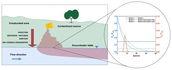
w0 have been calculated at a certain spatial location (z = 5 m) as a function of time, fixing a single contaminant, Trichloroethylene (TCE), soil type (sand), source thickness (L1 = 2 m). The results of the ratio between Cw/Cw0 are sketched in Figure 2.
As shown in Figure 2, the value of the initial dimensionless concentration and the shape of the curve are influenced by source hypotheses and transport mechanisms. According to these results, models belonging to group 1 (Model I and II) show a constant concentration over the time (with the exception of an initial transient phase for Model II); models belonging to group 2 (Model III and IV) show a decreasing exponential trend whereas models belonging to group 3 (Model V and VI) exhibit a temporal trend represented by a bell-shaped curve.
Model I is the most basic, as it neglects fate and transport mechanisms over time. Therefore, the dimensionless concentration Cw/Cw0 is constant. Conversely, Model II solves the transport equation, and it considers a constant source; therefore, at the initial time t = 0 the value of Cw/Cw0 is zero and after a transient phase reaches a constant value. Although both models showed a similar trend over the time, Model II depends on the spatial coordinates x, y, and z. The models belonging to group 1 can be used when the reduction processes of the source, like leaching and volatilization losses or biodegradation, are negligible, so the source can be modelled as constant. Pascuzzi et al. [71] used the model I for evaluating the risk for human health assuming a steady redeposition on the soil of pollutants in the selected site. The CW/CW0 was equal to 3.33 × 10⁻², while according to our results the CW/CW0 calculated through the application of the SAM coefficient ranges between 0.167 and 0.444. These different values are related to the differences in the adopted reference schemes, which cause a stronger attenuation process in the scheme presented by Pascuzzi et al. They consider a source thickness L1 of 0.2 m and a distance between the bottom of the source and the water table Lf equal to 6m, while in our case L1 ranges between 1 m and 4 m and Lf is 5 m.
Di Gianfilippo et al. [51] used Model I to reproduce the transport of leaching substances from alkaline waste material assuming a constant source. They carried out a Monte Carlo analysis to evaluate a wide range of scenario conditions, varying the input parameters within selected intervals. The SAM value was estimated using a value of L1 varying from 0.1 m to 1 m and a value of Lf from 5 to 10 m, thus obtaining a value of CW/CW0 ranging between 9.9 × 10⁻³ and 0.167. These concentrations are slightly lower than those calculated in this work because of the different geometrical conditions, as in the previous case.
The solutions of the group 2 consist of exponential laws, describing the depletion processes of the source. Model III assumes instantaneous mixing in the unsaturated zone, and it does not consider transport mechanisms. Therefore, Cw/Cw0 is spatially constant along the vertical axis, and it decreases over time. In Model IV the exponential law is multiplied by αleach. In this scenario, the value of αleach is approximately equal to 1, because of the selected type of soil and the contaminant. In consequence, the exponential part is dominant. The depletion coefficients μ1 and μ2 are equal to 3.469 × 10⁻⁹ s−1 and 4.800 × 10⁻⁹ s−1, respectively. They are indicators of the depletion rate of the contaminant and differ only for the retardation coefficient. Therefore, in these conditions, the results of the two models are very similar. For group 2, the source depletion processes (bio-chemical degradation and leaching losses) are predominant, while the transport mechanisms are less relevant.
Models V and VI can be considered as the more advanced ones as they consider both the source depletion and a transient transport equation. This causes the distinctive bell-shape, yielding a dimensionless concentration peak lower than the other models I-IV. The solutions contain two parts: a time-dependent exponential law and the space- and time-dependent solution of the transport equation. For Model V the first part takes into account only the biochemical degradation, while for Model VI, it considers leaching and volatilization losses. The second part of the solution is different due to the initial and boundary conditions of the transport equation. For these reasons, the peaks of the solutions differ between the Models V and VI. In this scenario, for Model V the maximum of the normalized concentration is 4.338 × 10⁻² at 8.17 y, while in Model VI, the maximum of the normalized concentration corresponds to 4.920 × 10⁻² at 8.08 y. These models allow to describe the fate and transport mechanisms more thoroughly than the other models. In this case, the predicted concentrations are approximately an order of magnitude lower than those obtained by using the other models.
For these reasons, in some applications, the models of these groups are preferable. Di Sante et al. [72] used Model VI to assess the sanitary and environmental risk of a disused industrial plant contaminated with polycyclic aromatic hydrocarbons, heavy hydrocarbons and polychlorinated biphenyls. Although the Italian guidelines [73] consider adequate a steady-state model to reproduce leaching phenomena, the authors suggest the use of a transient model for contaminants with high experimental leaching value, because they are more suitable to reproduce real conditions. They evaluated concentrations of aromatic fraction of heavy hydrocarbons and benzo(a)pyrene after 20 years roughly equal to 0.40 mg/L e 1 × 10⁻⁶ mg/L, respectively. Their results consider not only the leaching process but also the uniform dilution in groundwater, which is not considered by this paper. Furthermore, their results cannot be expressed as a dimensionless quantity. For these reasons, a direct comparison with the results of this work is not possible.
The different output concentrations of the models lead to different amounts of contaminant reaching the water table. In order to determine and compare the mass value reaching the groundwater for the different models, the mass flux (J) from unsaturated zone to groundwater is integrated over the time. J is governed only by water phase advection, and it is evaluated as suggested in [43]:
J = C w   A uz-gw   v leach
where Auz-gw is the exchange area between the two zones.
For all the models but Model II, Auz-gw is equal to A, and the dissolved concentration Cw is constant over the area. In the paper describing Model II [43], Auz-gw is bigger than A, and the concentration is variable in space; hence, it is necessary to integrate C(x,y,t) over space and time.
For the considered contaminant, soil type and source thickness, the mass reaching the water table, considering a period of twenty years and forty years, has been calculated starting from an initial source concentration Cw0 (100 μg/dm3); see Table 6. As can be noted, the third group of models returns a lower contaminant mass than the others. After 20 years, the exponential models belonging to group 2 exhibit the highest values, while extending the period of time to 40 years Model I exhibits the maximum value of J.

4.2. Predicted Concentration of Different Contaminants over Time

The physico-chemical characteristics of the contaminant, e.g., the volatility and the degradation rate [52,74], strongly affect its mobility through the unsaturated zone as well as its fate in time. The selected models are solved using the contaminants properties listed in Table 5, fixing the thickness of the source L1 = 2 m and a sand soil.
The transport time ranges between some orders of magnitude according to the contaminant mobility. Hence, in order to overcome this discrepancy and compare the results consistently, the dimensionless concentration has been plotted versus a dimensionless time τ, calculated as the ratio between the physical time and a reference time tref. This criterion has not been used for Model I because the results are not depended by time and contaminant properties. In this case, tref has not been considered, and the dimensionless concentration is plotted versus physical time. The value of the tref cannot be evaluated the same way for all the models. For models belonging to the groups 2 and 3, the dimensionless concentration goes to zero after a certain period of time, depending on contaminants and medium properties. Therefore, the value of tref has been set equal to the time when Cw/Cw0 reaches the residual value of 0.1%. For model II, the value of tref has been calculated with a different criterion, as in this case Cw/Cw0 tends to a horizontal asymptote: It is set equal to the time when the variation of the concentration is negligible (<0.01 μg/dm3). As one can perceive, in this case the value of tref depends on the temporal discretization, which has been set equal to 1 month for Benzene, Vinyl chloride and Trichloroethylene and 1 year for Benzo(a)pyrene and Aldrin.
The values of tref are listed in Table 7. It can be observed that Model III has the highest tref for all the contaminants. More generally, the models belonging to group 2 exhibit a higher tref than the other models for the contaminants characterized by a greater mobility (Benzene, Vinyl Chloride, and Trichloroethylene). For Benzo(a)pyrene and Aldrin, the reference time tref of Model V is not reported because Cw is negligible.
For the Model II (Figure 3b), it is possible to observe a marked distinction in the trend concentration between contaminants characterized by a less mobility (Benzo(a)pyrene and Aldrin) and the others (Benzene, Vinyl chloride, Trichloroethylene). The first group of contaminants reaches a steady-state concentration higher than the others: the Cw/Cw0 ratio is equal to 0.443 for Benzo(a)pyrene and 0.358 for Aldrin. The second group reaches lower values, the Cw/Cw0 ratio is about equal to 0.090 for the three contaminants. These results are in accordance with the application of the model presented by Locatelli et al. [75], considering the different hydrogeological setting of the simulated site. Locatelli et al. [75] used the model II to simulate leaching of benzene and toluene in a simulated contamination scenario; at 5 meters, they obtain a Cw/Cw0 ratio corresponding to 0.01 for benzene and 0.04 for toluene. The lower value compared to the obtained value in this paper can be attributed to the different hydrogeological setting and the different assessment of some parameters, like the degradation constant.
The Cw/Cw0 ratios for Benzo(a)pyrene and Aldrin in the Model II are higher than in Model I (Cw/Cw0 = 0.286). This proves that in some circumstances, the Model I is not the most conservative approach, as it is typically considered (ASTM, 2000). This result can be related to the fact that in Model I the SAM is assumed simplistically constant for all the contaminants.
In Model III, as can be seen from Figure 3c, the results collapse on the same curve as consequence of the use of the dimensionless time τ. This occurs in Model IV to some extent. In fact, as previously explained, Model IV consists of two terms: αdep and αleach. The former is characterized by scale invariance while the latter is approximately equal to one for all the contaminants. The minimum value of αleach corresponding to 0.930 has been obtained for Benzo(a)pyrene.
In Model V the concentrations of contaminants with low mobility (Benzo(a)pyrene and Aldrin) is closed to zero during the whole considered range of time (104–105 years) because of the exponential part of the solution. Therefore, the results of this model (Figure 3e) are shown only for the three contaminants Benzene, Vinyl Chloride and Trichloroethylene. In Figure 3f. sketching the results of Model VI, it is possible to identify two groups of contaminants, characterized by low and high mobility, respectively. The concentration of contaminants belonging to the first group reach a maximum value earlier than the second group.

Comparison between Different Degradation Constants

The contaminant degradation into the environment, λ, simulated through a first order kinetics, takes into account both chemical mechanisms (hydrolysis, redox reductions and photodegradations) and biodegradation. Several mechanisms are involved, and each of them can be affected by many environmental variables, making the assessments of these coefficients highly uncertain [76,77]. The λ values can vary by more than one order of magnitude for each contaminant in a natural porous media [15,78]. For these reasons, a sensitivity analysis based on the variation of λ has been carried out. The comparison is developed with respect to the Trichloroethylene compound, in the same conditions of the previous sections: depth equal to z = 5 m, source thickness L1 equal to 2 m and the unsaturated zone composed by sand. In Howard [66], the values of λ for Trichloroethylene in groundwater range from 4.852 × 10⁻⁹ s−1 to 2.499 × 10⁻⁸ s−1. Three values have then been chosen for the comparison: the first λ1 is the minimum value (4.852 × 10⁻⁹ s−1), the second λ2 is the mean of logarithms of the two extremes (1.101 × 10⁻⁹ s−1), and the third λ3 is the maximum value (2.499 × 10⁻⁸ s−1). The results of the comparison are shown in Figure 4.
As already highlighted, Model I is independent of contaminant properties; therefore, the ratio Cw/Cw0 is constant, equal to 0.286 for all the values of λ. In Model II (Figure 4b), little differences related to the decay coefficients can be noted. The obtained Cw/Cw0, equal to 0.0901, 0.0884 and 0.0848 for λ1, λ2 and λ3, respectively, present similar values, reaching the steady state conditions in a small period of time.
In the Models III and IV (Figure 4c,d), the λ coefficients play the same role, affecting the depletion coefficients μ1 and μ2, see Table 1.
The variation of λ affects Model V more than Model VI (Figure 4e,f). In particular, it influences the Cw/Cw0 peak (maximum concentration) as well as the time when it occurs. In both models, the higher is the value of λ, the earlier and lower is the peak. In Model V, Cw/Cw0 peaks correspond to 0.0438 at 8 y, 0.0094 at 7.83 y, 0.00033 at 7.42 y for the three values of λ considered, respectively, whereas in Model VI the Cw/Cw0 are equal to 0.0492 at 8.08 y, 0.0247 at 7.92 y and 0.0053 at 7.83 y.

4.3. Comparison between Different Soils

The physical properties of soil represent a further element that influences the fate and transport mechanisms of the contaminants. Simulations with three different soils (sand, loam, clay) have been carried out, in order to evaluate the corresponding differences in the models. Again, the comparison has been developed with respect to the Trichloroethylene compound in the same conditions depicted in the previous section. The three types of soils are characterized by the same organic carbon fraction, whereas they differ in grain size, water content, hydraulic conductivity and infiltration rate. The soil parameters values are listed in Table 4.
It is worth noting that the analyzed models consider the sorption process only through the soil-water partition coefficient, which is a synthetic parameter considering the characteristics of the soil, the contaminant and their interaction. This parameter should be assessed experimentally with reference to the specific soil-contaminant complex. In this analysis, it has been chosen to evaluate the partition coefficient referring only to the contaminant characteristics. For this reason, the obtained results for the different types of soils are affected only by the difference between hydrological characteristics of the soils, while the differences related to the sorption capacity are neglected. This assumption has resulted in a lower partition coefficient value of the clays than the experimental values in these soils and, consequently, a higher value of the simulated contaminant concentration. Clay soils have, in fact, a higher sorption behavior than the other soils because of the high surface area and negative charged sites of the soils particles.
As previously seen, Model I is independent by the soil parameters (Figure 5a). Model II (Figure 5b) shows a similar behavior for sand and loam, reaching the steady state Cw/Cw0 ratios corresponding to 0.0902 and 0.0836, at 1.67 y and 2.42 y respectively. A lower mobility could be observed for clay. In this case the steady concentration, Cw/Cw0 equal to 0.0538, is reached at t = 7.67 y. Hence, the leaching velocity has a greater impact compared to the sorption capacity.
Model III and IV give similar trends as shown in Figure 5c,d, respectively. In Model III, the time needed to reach the 0.1% of the initial concentration, is equal to 63.17 y, 72.67 y, 69.83 y whereas, in Model IV the time needed to reach the 0.1% of the initial concentration is equal to 45.67 y, 63.00 y and 68.58 y for sand, clay and loam, respectively.
Models V and VI are most influenced by soil parameters, which affect both the time at which the maximum concentration occurs at z = 5 m and the related values. The transport mechanism lasts very long when Model V is applied for clay. Hence the concentration is so extremely low and therefore undetectable. The Cw/Cw0 peaks are equal to 4.380 × 10⁻² at 8 y and 8.651 × 10⁻³ at 18.67 y in sand and loam, respectively. In Model VI the peaks are of the same order of magnitude for sand and loam, whereas it is negligible for clay. In this case, the Cw/Cw0 ratios are equal to 4.920 × 10⁻² at 8.08 y and 1.509 × 10⁻² at 19.75 y for sand and loam, respectively.

4.4. Comparison between Different Source Thickness

As can be seen in Table 1, the thickness of the source L1 determines the soil attenuation of the contaminant in the Model I, and the time needed to deplete the source in the models composed of an exponential part (Models III to VI). Model II is not influenced by the change of source thickness because it does not take into account the source depletion and soil attenuation. The simulations have been carried out taking into account the scheme depicted in Figure 1, with three different source depths: L1 = 1 m, 2 m and 4 m, using sand as type of soil and Trichloroethylene as contaminant. Again, the dimensionless concentration Cw/Cw0 has been calculated at the depth z = 5 m. The concentrations calculated with Model I (Figure 6a) shows a significant variation in relation to the source thickness, being equal to 0.167, 0.286 and 0.444, for L1 equal to 1 m, 2 m, 4 m respectively.
In the exponential Models III and IV (Figure 6c,d), the source thickness has a different effect. The depletion coefficients μ1 and μ2 (Table 1) may be used as indicators of the contaminant depletion velocity. The time needed to reach the 0.1% of the initial concentration increases with thickness, reaching the values of 58, 64 and 73 years in the Model III. In Model IV the time needed to reach the 0.1% of the initial concentration is equal to 27, 46 and 70 years for the three values of L1.
In the Model V, an increased thickness of the source determines delayed and higher peaks. The Cw/Cw0 ratios are 2.25 × 10⁻² (t = 7.92 y), 4.38 × 10⁻² (t = 8.00 y) and 8.24 × 10⁻² (t = 8.25 y) for L1 equal to 1 m, 2 m, 4 m respectively.
In the Model VI, the increasing of the source thickness lead to higher but earlier peaks. The Cw/Cw0 ratios are equal to 3.19 × 10⁻² (t = 8.08 y), 4.92 × 10⁻² (t = 8.08 y) and 7.93 × 10⁻² (t = 8.00 y), for L1 equal to 1 m, 2 m, 4 m respectively.

5. Conclusions

The use of fate and transport models may give a considerable support to tackle with environmental problems involving chemical leaching in the vadose zone. Unlike numerical based approaches, analytical models are used especially in the risk assessment of contaminants due to their straightforward application and simplicity. Six analytical models, reproducing contaminant fate and transport from a source located in the unsaturated zone to the groundwater were described and compared with the aim of giving some insights about their use.
On the basis of their characteristics three groups were identified. The first one is suited for contamination scenarios where the source may be assumed constant, e.g. in the case of continuous chemicals leakage. The second group is particularly appropriate when the depletion processes are predominant and the travel distance of the chemical is low, e.g. a localized spill of biodegradable organic contaminant near the water table. The third group describes more comprehensively all the processes occurring during the transport.
Simulations being carried out, showed that models belonging to the third group yielded lowest values of contaminant concentration with respect to the other models, giving the less conservative results. When a more conservative approach is needed, Models I to IV should be preferred instead.
Future research could be addressed to either enhance the existing analytical models or to propose new advanced ones, while preserving their suitability for engineering applications, in order to obtain a more realistic representation of contaminant fate and transport in the unsaturated zone.

Author Contributions

Conceptualization, M.G.S., G.L., M.C., G.V., C.G., and L.C.; methodology, M.G.S., G.L. and M.C.; formal analysis, M.G.S., G.L. and M.C.; investigation, M.G.S., G.L., M.C., G.V. and C.G.; resources, G.V.; data curation, M.G.S.; writing—original draft preparation, M.G.S., G.L., M.C. and G.V.; visualization, M.G.S.; supervision, G.L., M.C., G.V., C.G., and L.C. All authors have read and agreed to the published version of the manuscript.

Funding

This research received no external funding.

Conflicts of Interest

The authors declare no conflict of interest.

Nomenclature

AHorizontal source area (m2)
Auz-gwExchange area between the unsaturated zone and the groundwater (m2)
CaSoil gas concentration (mg m−3)
CNAPLConcentration in non-aqueous phase (mg kg−1)
CsConcentration of the chemical sorbed by the soil (mg kg−1)
CtotTotal source concentration (mg kg−1)
Ctot;satTotal source concentration equivalent to saturation conditions (mg kg−1)
CwDissolved concentration in pore water (mg m−3)
Cw0Initial dissolved concentration in pore water at the source (mg m−3)
DDispersion tensor of Model II (m2 s−1)
D′xDispersion parameter of Model II in x-direction (m2 s−1)
D′yDispersion parameter of Model II in y-direction (m2 s−1)
D′zDispersion parameter of Model II in z-direction (m2 s−1)
DaDiffusion tensor in air (m2 s−1)
Da0Diffusion coefficient in air (m2 s−1)
DaePore diffusion coefficient in air (m2 s−1)
DeffEffective diffusion coefficient according Millington and Quirk relationship (m2 s−1)
DwDispersion tensor in (m2 s−1)
Dw0Diffusion coefficient in water (m2 s−1)
DwePore diffusion coefficient in water (m2 s−1)
DzDispersion-diffusion coefficient in water in z-direction (m2 s−1)
focOrganic carbon fraction
HDimensionless Henry’s constant
hcrWetting front suction head (m)
HwPonding depth of water surface (m)
IeffEffective infiltration (m s−1)
JMass flux from unsaturated zone to groundwater (m s−1)
KdSoil sorbed-water partition coefficient (m3 kg−1)
KocOrganic carbon-water partition coefficient (m3 kg−1)
KsatSaturated hydraulic conductivity (m s−1)
KswTotal soil-water partition coefficient (kg m−3)
L1Thickness of the contaminant source (m)
L2Distance between the top of the source and the water table (m)
LdDiffusion path length (m)
LDFLeachate-groundwater dilution factor
LfDistance between the bottom of the source and the water table (m)
LFLeachate factor
MaContaminant mass in vapour phase (kg)
MsContaminant mass sorbed by the soil fraction (kg)
MsatTotal contaminant mass equivalent to saturation conditions (kg)
MtotTotal contaminant mass (kg)
MwContaminant mass in water phase (kg)
RRetardation coefficient
RRetardation parameter of Model II
SSolubility (kg m−3)
SAMSoil attenuation model
t0Initial time (s)
t*Time when the initial source concentration reaches the saturation conditions in Model IV (s)
tleachTime required for the contaminant to reach the underlying water table in Model IV (s)
twTime required for infiltrating water to reach the water table in Model IV (s)
tPhysical time (approximation ±1month)
vVelocity parameter of Model II (m s−1)
vSeepage velocity (m s−1)
XLength of the contaminant source (m)
xHorizontal spatial coordinate-1 (m)
YWidth of the contaminant source (m)
yHorizontal spatial coordinate-2 (m)
zVertical spatial coordinate (m)
z0Thickness of slug in Model V (m)
zmDistance from the source to the observation location (m)
αdepSource depletion factor in Model IV
αlLongitudinal dispersivities in the water phase (m)
αleachLeaching factor in Model IV
αtTransverse dispersivities in the water phase (m)
λFirst order degradation constant (s−1)
λParameter of Model II (s−1)
μ1Depletion coefficient in Model III (s−1)
μ2Depletion coefficient in Model IV (s−1)
μ3Depletion coefficient in Model VI (s−1)
θPorosity
θaVolumetric air content
θwVolumetric water content
ρbSoil bulk density (kg m−3)
τDimensionless time

References

  1. Barnes, K.K.; Kolpin, D.W.; Furlong, E.T.; Zaugg, S.D.; Meyer, M.T.; Barber, L.B. A national reconnaissance of pharmaceuticals and other organic wastewater contaminants in the United States —I) Groundwater. Sci. Total Environ. 2008, 402, 192–200. [Google Scholar] [CrossRef] [PubMed]
  2. Focazio, M.J.; Kolpin, D.W.; Barnes, K.K.; Furlong, E.T.; Meyer, M.T.; Zaugg, S.D.; Barber, L.B.; Thurman, M.E. A national reconnaissance for pharmaceuticals and other organic wastewater contaminants in the United States—II) Untreated drinking water sources. Sci. Total Environ. 2008, 402, 201–216. [Google Scholar] [CrossRef] [PubMed]
  3. Postigo, C.; Barceló, D. Synthetic organic compounds and their transformation products in groundwater: Occurrence, fate and mitigation. Sci. Total Environ. 2015, 503, 32–47. [Google Scholar] [CrossRef] [PubMed]
  4. Yadav, I.C.; Devi, N.L.; Syed, J.H.; Cheng, Z.; Li, J.; Zhang, G.; Jones, K.C. Current status of persistent organic pesticides residues in air, water, and soil, and their possible effect on neighboring countries: A comprehensive review of India. Sci. Total Environ. 2015, 511, 123–137. [Google Scholar] [CrossRef] [PubMed]
  5. Lesser, L.E.; Mora, A.; Moreau, C.; Mahlknecht, J.; Hernández-Antonio, A.; Ramírez, A.I.; Barrios-Pina, H. Survey of 218 organic contaminants in groundwater derived from the world’s largest untreated wastewater irrigation system: Mezquital Valley, Mexico. Chemosphere 2018, 198, 510–521. [Google Scholar] [CrossRef] [PubMed]
  6. Graber, E.R.; Laor, Y.; Ronen, D. Aquifer contamination by chlorinated-VOCs: The case of an urban metropolis megasite overlying the Coastal Plain aquifer in Israel. Hydrogeol. J. 2008, 16, 1615–1623. [Google Scholar] [CrossRef]
  7. Schaider, L.A.; Rudel, R.A.; Ackerman, J.M.; Dunagan, S.C.; Brody, J.G. Pharmaceuticals, perfluorosurfactants, and other organic wastewater compounds in public drinking water wells in a shallow sand and gravel aquifer. Sci. Total Environ. 2014, 468, 384–393. [Google Scholar] [CrossRef] [Green Version]
  8. Lehosmaa, K.; Jyväsjärvi, J.; Ilmonen, J.; Rossi, P.M.; Paasivirta, L.; Muotka, T. Groundwater contamination and land drainage induce divergent responses in boreal spring ecosystems. Sci. Total Environ. 2018, 639, 100–109. [Google Scholar] [CrossRef] [PubMed]
  9. Wang, Q.; Kelly, B.C. Assessing bioaccumulation behaviour of hydrophobic organic contaminants in a tropical urban catchment. J. Hazard. Mater. 2018, 358, 366–375. [Google Scholar] [CrossRef] [PubMed]
  10. Foster, S.; Hirata, R.; Gomes, D.; D’Elia, M.; Paris, M. Groundwater Quality Protection: A Guide for Water Service Companies, Municipal Authorities and Environment Agencies; The World Bank: Washington, DC, USA, 2002. [Google Scholar] [CrossRef]
  11. Šimůnek, J.; van Genuchten, M.T. Contaminant transport in the unsaturated zone: Theory and modeling. In The Handbook of Groundwater Engineering, 3rd ed.; CRC Press: Boca Raton, FL, USA, 2016; pp. 221–254. ISBN 9781498703055. [Google Scholar]
  12. Praseeja, A.V.; Sajikumar, N. A review on the study of immiscible fluid flow in unsaturated porous media: Modeling and remediation. J. Porous Media 2019, 22, 889–922. [Google Scholar] [CrossRef]
  13. Luo, Y.; Gao, Q.; Yang, X. Dynamic modeling of chemical fate and transport in multimedia environments at watershed scale-I: Theoretical considerations and model implementation. J. Environ. Manag. 2007, 83, 44–55. [Google Scholar] [CrossRef] [PubMed]
  14. Swartjes, F.A.; Rutgers, M.; Lijzen, J.P.A.; Janssen, P.J.C.M.; Otte, P.F.; Wintersen, A.; Brand, E.; Posthuma, L. State of the art of contaminated site management in The Netherlands: Policy framework and risk assessment tools. Sci. Total Environ. 2012, 427, 1–10. [Google Scholar] [CrossRef] [PubMed]
  15. Nham, H.T.T.; Greskowiak, J.; Nödler, K.; Rahman, M.A.; Spachos, T.; Rusteberg, B.; Massmann, G.; Sauter, M.; Licha, T. Modeling the transport behavior of 16 emerging organic contaminants during soil aquifer treatment. Sci. Total Environ. 2015, 514, 450–458. [Google Scholar] [CrossRef] [PubMed]
  16. Pullan, S.P.; Whelan, M.J.; Rettino, J.; Filby, K.; Eyre, S.; Holman, I.P. Development and application of a catchment scale pesticide fate and transport model for use in drinking water risk assessment. Sci. Total Environ. 2016, 563, 434–447. [Google Scholar] [CrossRef] [Green Version]
  17. Mohanadhas, B.; Kumar, G.S. Numerical Experiments on Fate and Transport of Benzene with Biological Clogging in Vadoze Zone. Environ. Process. 2019, 6, 841–858. [Google Scholar] [CrossRef]
  18. Huan, H.; Wang, J.; Zhai, Y.; Xi, B.; Li, J.; Li, M. Quantitative evaluation of specific vulnerability to nitrate for groundwater resource protection based on process-based simulation model. Sci. Total Environ. 2016, 550, 768–784. [Google Scholar] [CrossRef]
  19. Trulli, E.; Morosini, C.; Rada, E.C.; Torretta, V. Remediation in Situ of Hydrocarbons by Combined Treatment in a Contaminated Alluvial Soil due to an Accidental Spill of LNAPL. Sustainability 2016, 8, 1086. [Google Scholar] [CrossRef] [Green Version]
  20. Alexander, A.C.; Ndambuki, J.M.; Salim, R.W.; Manda, A.K. Groundwater remediation optimization using Solving Constraint Integer Program (SCIP). Groundw. Sustain. Dev. 2018, 7, 176–184. [Google Scholar] [CrossRef]
  21. O’Brien, P.L.; DeSutter, T.M.; Casey, F.X.M.; Khan, E.; Wick, A.F. Thermal remediation alters soil properties–A review. J. Environ. Manag. 2018, 206, 826–835. [Google Scholar] [CrossRef]
  22. Tsakiroglou, C.D.; Sikinioti-Lock, A.; Terzi, K.; Theodoropoulou, M. A numerical model to simulate the NAPL source zone remediation by injecting zero-valent iron nanoparticles. Chem. Eng. Sci. 2018, 192, 391–413. [Google Scholar] [CrossRef]
  23. Falciglia, P.P.; Scandura, P.; Vagliasindi, F.G.A. Modelling and preliminary technical, energy and economic considerations for full-scale in situ remediation of low-dielectric hydrocarbon-polluted soils by microwave heating (MWH) technique. J. Soil Sediment 2018, 18, 2350–2360. [Google Scholar] [CrossRef]
  24. Singh, G.; Kaur, G.; Williard, K.; Schoonover, J.; Kang, J. Monitoring of water and solute transport in the vadose zone: A review. Vadose Zone J. 2018, 17, 160058. [Google Scholar] [CrossRef]
  25. Fiorentino, A.; De Luca, G.; Rizzo, L.; Viccione, G.; Lofrano, G.; Carotenuto, M. Simulating the fate of indigenous antibiotic resistant bacteria in a mild slope wastewater polluted stream. J. Environ. Sci. 2018, 69, 95–104. [Google Scholar] [CrossRef]
  26. Karapanagioti, H.K.; Gaganis, P.; Burganos, V.N. Modeling attenuation of volatile organic mixtures in the unsaturated zone: Codes and usage. Environ. Modell. Softw. 2003, 18, 329–337. [Google Scholar] [CrossRef]
  27. Dafny, E. TCE longevity in the vadose zone and loading to the groundwater—The case of episodic NAPL releases from near-surface source. Environ. Technol. Innov. 2017, 7, 128–140. [Google Scholar] [CrossRef]
  28. Sudicky, E.A.; Hwang, H.T.; Illman, W.A.; Wu, Y.S.; Kool, J.B.; Huyakorn, P. A semi-analytical solution for simulating contaminant transport subject to chain-decay reactions. J. Contam. Hydrol. 2013, 144, 20–45. [Google Scholar] [CrossRef]
  29. Guan, C.; Xie, H.J.; Wang, Y.Z.; Chen, Y.M.; Jiang, Y.S.; Tang, X.W. An analytical model for solute transport through a GCL-based two-layered liner considering biodegradation. Sci. Total Environ. 2014, 466, 221–231. [Google Scholar] [CrossRef] [PubMed]
  30. Moranda, A.; Cianci, R.; Paladino, O. Analytical Solutions of One-Dimensional Contaminant Transport in Soils with Source Production-Decay. Soil Syst. 2018, 2, 40. [Google Scholar] [CrossRef] [Green Version]
  31. Mao, X.; Prommer, H.; Barry, D.A.; Langevin, C.D.; Panteleit, B.; Li, L. Three-dimensional model for multi-component reactive transport with variable density groundwater flow. Environ. Model. Softw. 2006, 21, 615–628. [Google Scholar] [CrossRef]
  32. Wu, S.; Jeng, D.S. Numerical modeling of solute transport in deformable unsaturated layered soil. Water Sci. Eng. 2017, 10, 184–196. [Google Scholar] [CrossRef]
  33. Mohamed, A.M.O.; Paleologos, E.K.; Singh, D.N.; Rodrigues, V.S. Chapter 9-Subsurface Contaminant Transport. In Fundamentals of Geoenvironmental Engineering; Butterworth-Heinemann: Oxford, UK, 2017. [Google Scholar] [CrossRef]
  34. Paladino, O.; Moranda, A.; Massabò, M.; Robbins, G.A. Analytical Solutions of Three-Dimensional Contaminant Transport Models with Exponential Source Decay. Groundwater 2018, 56, 96–108. [Google Scholar] [CrossRef] [PubMed]
  35. Anderson, M.P.; Woessner, W.W.; Hunt, R.J. Applied Groundwater Modeling: Simulation of Flow and Advective Transport, 2nd ed.; Academic Press: Amsterdam, The Netherlands, 2015; ISBN 9780120581030. [Google Scholar]
  36. Mazzieri, F.; Di Sante, M.; Fratalocchi, E.; Pasqualini, E. Modeling contaminant leaching and transport to groundwater in Tier 2 risk assessment procedures of contaminated sites. Environ. Earth Sci. 2016, 75, 1247. [Google Scholar] [CrossRef]
  37. Feyen, J.; Jacques, D.; Timmerman, A.; Vanderborght, J. Modelling water flow and solute transport in heterogeneous soils: A review of recent approaches. J. Agric. Eng. Res. 1998, 70, 231–256. [Google Scholar] [CrossRef] [Green Version]
  38. Vanclooster, M.; Javaux, M.; Vanderborght, J. Solute Transport in Soil at the Core and Field Scale. Encycl. Hydrol. Sci. 2006. [Google Scholar] [CrossRef]
  39. Rivett, M.O.; Wealthall, G.P.; Dearden, R.A.; McAlary, T.A. Review of unsaturated-zone transport and attenuation of volatile organic compound (VOC) plumes leached from shallow source zones. J. Contam. Hydrol. 2011, 123, 130–156. [Google Scholar] [CrossRef]
  40. Šimůnek, J. Models of water flow and solute transport in the unsaturated zone. Encycl. Hydrol. Sci. 2006. [Google Scholar] [CrossRef]
  41. Nolan, B.T.; Bayless, E.R.; Green, C.T.; Garg, S.; Voss, F.D.; Lampe, D.C.; Barbash, J.E.; Capel, P.D.; Bekins, B.A. Evaluation of Unsaturated-zone Solute-Transport Models for Studies of Agricultural Chemicals; No. USGS-OFR-2005-1196; Geological Survey: Reston, VA, USA, 2005.
  42. ASTM. Standard Guide for Risk-Based Corrective Action; ASTM: West Conshocken, PA, USA, 2000. [Google Scholar]
  43. Troldborg, M.; Binning, P.J.; Nielsen, S.; Kjeldsen, P.; Christensen, A.G. Unsaturated zone leaching models for assessing risk to groundwater of contaminated sites. J. Contam. Hydrol. 2009, 105, 28–37. [Google Scholar] [CrossRef]
  44. Troldborg, M.; Lemming, G.; Binning, P.J.; Tuxen, N.; Bjerg, P.L. Risk assessment and prioritisation of contaminated sites on the catchment scale. J. Contam. Hydrol. 2008, 101, 14–28. [Google Scholar] [CrossRef] [PubMed]
  45. Verginelli, I.; Baciocchi, R. Role of natural attenuation in modeling the leaching of contaminants in the risk analysis framework. J. Environ. Manag. 2013, 114, 395–403. [Google Scholar] [CrossRef]
  46. Enfield, C.G.; Carsel, R.F.; Cohen, S.Z.; Phan, T.; Walters, D.M. Approximating Pollutant Transport to Ground Water. Groundwater 1982, 20, 711–722. [Google Scholar] [CrossRef]
  47. Spence, L.; Walden, T. Risk Integrated Software for Cleanups: RISC4 User’s Manual; Spence Engineering: Pleasant, CA, USA, 2001. [Google Scholar]
  48. Meza, J.C.S.; Perez, P.A.; Salin, M.B.; Salazar, V.F.P.; Lapoint, T. Inhibition of cholinesterase activity by soil extracts and predicted environmental concentrations (PEC) to select relevant pesticides in polluted soils. J. Environ. Sci. Health B 2010, 45, 214–221. [Google Scholar] [CrossRef] [PubMed]
  49. Jennings, A.A.; Li, Z. Scope of the worldwide effort to regulate pesticide contamination in surface soils. J. Environ. Manag. 2014, 146, 420–443. [Google Scholar] [CrossRef] [PubMed]
  50. Di Sante, M.; Mazzieri, F.; Fratalocchi, E.; Brianzoni, V.; Pasqualini, E. A possible approach for Tier 2 risk assessments of polluted sites: Framework, computer spreadsheet and application. Comput. Geotech. 2014, 56, 16–27. [Google Scholar] [CrossRef]
  51. Di Gianfilippo, M.; Verginelli, I.; Costa, G.; Spagnuolo, R.; Gavasci, R.; Lombardi, F. A risk-based approach for assessing the recycling potential of an alkaline waste material as road sub-base filler material. Waste Manag. 2018, 71, 440–453. [Google Scholar] [CrossRef] [PubMed]
  52. Mulligan, C.N.; Yong, R.N. Natural attenuation of contaminated soils. Environ. Int. 2004, 30, 587–601. [Google Scholar] [CrossRef] [PubMed]
  53. Connor, J.A.; Bowers, R.L.; McHugh, T.; Spexet, A. Software Guidance Manual RBCA Tool Kit for Chemical Releases; GSI Environmental Inc.: Houston, TX, USA, 2007; pp. 1–120. [Google Scholar]
  54. Moldrup, P.; Olesen, T.; Komatsu, T.; Schjønning, P.; Rolston, D.E. Tortuosity, diffusivity, and permeability in the soil liquid and gaseous phases. Soil Sci. Soc. Am. J. 2001, 65, 613–623. [Google Scholar] [CrossRef]
  55. Sagar, B. Dispersion in three dimensions: Approximate analytic solutions. J. Hydraul. Eng. Div. ASCE 1982, 108, 47–62. [Google Scholar]
  56. Wexler, E.J. Analytical Solutions for One-, Two-, and Three-Dimensional Solute Transport in Ground-Water Systems with Uniform Flow; USGS Numbered Series; US Government Printing Office: Washington, DC, USA, 1989; pp. 89–156. [CrossRef]
  57. Green, W.H.; Ampt, G.A. Studies on Soil Phyics. J. Agric. Sci. 1911, 4, 1–24. [Google Scholar] [CrossRef] [Green Version]
  58. Ravi, V.; Johnson, J.A. PESTAN: Pesticide Analytical Model Version 4.0 User’s Guide; U.S. Environmental Protection Agency (EPA): Washington, DC, USA, 1992.
  59. Biggar, J.W.; Nielsen, D.R. Spatial variability of the leaching characteristics of a field soil. Water Resour. Res. 1976, 12, 78–84. [Google Scholar] [CrossRef]
  60. Ünlü, K.; Kemblowski, M.W.; Parker, J.C.; Stevens, D.; Chong, P.K.; Kamil, I. A screening model for effects of land-disposed wastes on groundwater quality. J. Contam. Hydrol. 1992, 11, 27–49. [Google Scholar] [CrossRef]
  61. Millington, R.J.; Quirk, J.P. Permeability of porous solids. T. Faraday Soc. 1961, 57, 1200–1207. [Google Scholar] [CrossRef]
  62. Gelhar, L.W. A Review of Field-Scale Physical Solute Transport Processes in Saturated and Unsaturated Porous Media; EA-4190. Res. Proj. 2485-5; Electric Power Research Institute: Palo Alto, CA, USA, 1985. [Google Scholar]
  63. Carsel, R.F.; Parrish, R.S. Developing joint probability distributions of soil water retention characteristics. Water Resour. Res. 1988, 24, 755–769. [Google Scholar] [CrossRef] [Green Version]
  64. Connor, J.A.; Newell, C.J.; Malander, M.W. Parameter estimation guidelines for risk-based corrective action (RBCA) modeling. In Proceedings of the Petroleum Hydrocarbons and Organic Chemicals in Groundwater Conference, Houston, TX, USA, 13–15 November 1996; pp. 13–15. [Google Scholar]
  65. Soil Screening Guidance: Technical Background Document; Office of Solid Waste and Emergency Response, U.S. Environmental Protection Agency (EPA): Washington, DC, USA, 1996.
  66. Howard, P.H. Handbook of Environmental Degradation Rates; CRC Press: Boca Raton, FL, USA, 2017; ISBN 9780873713580. [Google Scholar]
  67. Hallberg, G.R. Pesticides pollution of groundwater in the humid United States. Agric. Ecosyst. Environ. 1989, 26, 299–367. [Google Scholar] [CrossRef]
  68. Schiefler, A.A.; Tobler, D.J.; Overheu, N.D.; Tuxen, N. Extent of natural attenuation of chlorinated ethenes at a contaminated site in Denmark. Energy Procedia 2018, 146, 188–193. [Google Scholar] [CrossRef]
  69. Shao, Y.; Wang, Y.; Xu, X.; Wu, X.; Jiang, Z.; He, S.; Qian, K. Occurrence and source apportionment of PAHs in highly vulnerable karst system. Sci. Total Environ. 2014, 490, 153–160. [Google Scholar] [CrossRef] [PubMed]
  70. Vanderborght, J.; Vereecken, H. Review of dispersivities for transport modeling in soils. Vadose Zone J. 2007, 6, 29–52. [Google Scholar] [CrossRef]
  71. Pascuzzi, S.; Russo, G.; Scarascia-Mugnozza, G.; Verdiani, G.; Lagattolla, G. Contamination of the Environmental Matrices in Agricultural Areas Produced by Industrial Discharges: The Case Study of the Land of the City of Statte (Taranto, Southern Italy). Procedia Environ. Sci. 2013, 19, 671–680. [Google Scholar] [CrossRef] [Green Version]
  72. Di Sante, M.; Mazzieri, F.; Pasqualini, E. Assessment of the sanitary and environmental risks posed by a contaminated industrial site. J. Hazard. Mater. 2009, 171, 524–534. [Google Scholar] [CrossRef]
  73. ISPRA. Criteri Metodologici per l’applicazione dell’analisi Assoluta di Rischio ai siti Contaminati. In ECOMONDO 2005; MAGGIOLI: Rome, Italy, 2008; Volume 2. (In Italian) [Google Scholar]
  74. Weber, W.J., Jr.; McGinley, P.M.; Katz, L.E. Sorption phenomena in subsurface systems: Concepts, models and effects on contaminant fate and transport. Water Res. 1991, 25, 499–528. [Google Scholar] [CrossRef] [Green Version]
  75. Locatelli, L.; Rosenberg, L.; Bjerg, P.L.; Binning, P.J. GrundRisk-Coupling of Vertical and Horizontal Transport Models; Ministery of Environment and Food of Denmark: København, Denmark, 2017.
  76. McLachlan, M.S.; Zou, H.; Gouin, T. Using Benchmarking To Strengthen the Assessment of Persistence. Environ. Sci. Technol. 2016, 51, 4–11. [Google Scholar] [CrossRef]
  77. Viccione, G.; Stoppiello, M.G.; Lauria, S.; Cascini, L. Numerical Modelling of Contaminant Fate and Transport in the Vadose Zone. MDPI Proceedings. Available online: https://www.mdpi.com/journal/proceedings (accessed on 10 March 2020).
  78. Greskowiak, J.; Hamann, E.; Burke, V.; Massmann, G. The uncertainty of biodegradation rate constants of emerging organic compounds in soil and groundwater–A compilation of literature values for 82 substances. Water Res. 2017, 126, 122–133. [Google Scholar] [CrossRef] [PubMed]
Figure 1. Reference scheme.
Sustainability 12 02949 g001
Figure 2. Predicted dimensionless concentration Cw/Cw0 of TCE at z = 5 m according to the selected properties and models versus time. Results of Model V and VI are scaled by making use of the secondary axis.
Sustainability 12 02949 g002
Figure 3. Predicted dimensionless concentration Cw/Cw0 versus dimensionless time τ, at z = 5, for different contaminants. (a) Model I, (b) Model II, (c) Model III, (d) Model IV, (e) Model V, (f) Model VI.
Sustainability 12 02949 g003
Figure 4. Predicted Dimensionless concentration Cw/Cw0 of TCE at z = 5, m for different decay coefficients λ. (a) Model I, (b) Model II, (c) Model III, (d) Model IV, (e) Model V, (f) Model VI.
Sustainability 12 02949 g004
Figure 5. Predicted dimensionless concentration Cw/Cw0 of TCE at z = 5 m, for different soils: (a) Model I, (b) Model II, (c) Model III, (d) Model IV, (e) Model V, (f) Model VI.
Sustainability 12 02949 g005
Figure 6. Predicted dimensionless concentration Cw/Cw0 of TCE at z = 5 m, for different source thickness L1. (a) Model I, (b) Model II, (c) Model III, (d) Model IV, (e) Model V, (f) Model VI.
Sustainability 12 02949 g006
Table 1. Analytical solutions of the selected models.
GroupModelBoundary and Initial ConditionsSolutionReference
1I(-) C w ( z = L f ) = S A M · C w 0
       S A M = L 1 L f + L 1
ASTM, 2000 [42]
II C w ( z , x , y , 0 ) = 0   
0 < z <   < x <   
< y <
C w ( 0 , x , y , t ) = { C w 0 X 2 < x < X 2 , Y 2 < y < Y 2 0 o t h e r w i s e
C w ( z , x , y , t ) = C w 0 8 τ = 0 τ = t f z ( z , τ ) f x ( x , τ ) f y ( y , τ ) d τ
f z ( z , τ ) = z π D z e x p ( v z 2 D z ) · e x p [ τ ( ( v ) 2 4 D z + λ ) z 2 4 D z τ ] · τ 3 2
f x ( x , τ ) = { e r f [ x + X 2 2 D x τ ] e r f [ x X 2 2 D x τ ] }
f y ( y , τ ) = { e r f [ y + Y 2 2 D y τ ] e r f [ y Y 2 2 D y τ ] }
Troldborg et al., 2009 [43]
2III(-) C w ( t ) = C w 0 exp ( μ 1 t )
μ 1 = θ W θ W + ρ b K d + H θ a ( I e f f L 2 θ W + λ )
Troldborg et al., 2008 [44]
IV C w ( z = 0 ) = C w 0
d 2 C w d z 2 ( z = L f ) = 0
C w ( z , t ) = C w 0 · α d e p ( t ) · α l e a c h
α d e p ( t ) = exp ( μ 2 · t )   
μ 2 = I e f f · K s w R · L 1 · ρ s + λ s o u r c e · θ w · K s w ρ s
      α l e a c h = σ · exp ( k · z ) k · sinh ( σ · z ) + σ · cosh ( σ · z )
    k = z 2 · D · t l e a c h     σ = k 2 + λ · θ w D
Verginelli and Baciocchi, 2013 [45]
3V C w ( z , t = 0 ) = { 0 < z < z 0 C w 0 z 0 < z < 0 0 0 < z <
lim z C w z = 0
C w ( z , t ) = C w 0 2 exp ( λ t ) { e r f [ z + z 0 v   t R 2 D t R ] e r f [ z v   t R 2 D t R ] } Enfield et al., 1982 [46]
VI C w ( z , 0 ) = 0
C w ( 0 , t ) = C w 0 exp ( μ 3 t )
C w z ( , t ) = 0
C w ( z , t ) = C w 0 exp ( μ 3 t ) 1 2 e x p [ ( v w ) z 2 D z ] e r f c [ z R w t 2 D z R t ] + 1 2 e x p [ ( v + w ) z 2 D z ] e r f c [ z R + w t 2 D z R t ]
w = v ¯ 1 + 4 D z R v 2 [ λ μ 3 ]
μ 3 = I e f f K s w L 1 ρ b + D e f f H ρ b L 1 L d
Spence & Walden, 2001 [47]
Table 2. Features of the selected models.
GroupModelSourceChemical-Physical Mechanisms during the TransportSolve Transport Equation
On Ground SurfaceInner DomainContinuousTime-VaryingResidual NAPL PhaseAdvectionDispersion-Diffusion in WaterDiffusion in GasSorptionDegradation
1I xx x x
II xx xx (3D)x (3D)xxx
2III x xxx
IV x xxxx (1D) xxx (steady state)
3Vx x xx (1D) xxx
VI x xxxx (1D) xxx
Table 3. Values of the geometrical parameters.
Parameter *Value
L11-2-4 m
X4 m
Y4 m
Lf5 m
* See nomenclature list.
Table 4. Soil parameters values.
Parameter *Measurement UnitSandLoamClay
ρbkg/m3170017001700
θ-0.3850.3520.312
θw-0.1300.2000.304
θa-0.3000.2300.076
hcrm−0.0164−0.178−0.269
Iefm/s5.708 × 10−92.854 × 10−95.708 × 10−10
Ksatm/s8.250 × 10−52.889 × 10−65.556 × 10−7
foc-0.0010.0010.001
* See nomenclature list.
Table 5. Physico-chemical properties values of the selected contaminants.
Parameter *Measurement UnitContaminant
BenzeneBenzo(a)pyreneVinyl ChlorideTrichloroethyleneAldrin
H-2.280 × 10−14.630 × 10−51.1104.220 × 10−16.970 × 10⁻³
Skg/m31.7501.620 × 10−62.7601.1001.800 × 10−4
Dam2/s8.800 × 10−64.300 × 10−61.060 × 10−57.900 × 10−61.320 × 10−4
Dwm2/s9.800 × 10−109.000 × 10−101.230 × 10−109.100 × 10−104.860 × 10⁻¹⁰
Kocm3/kg6.170 × 10−29.690 × 1021.860 × 10−29.430 × 10−24.870 × 101
λ1/s1.114 × 10−87.567 × 10−92.790 × 10−94.852 × 10−96.778 × 10−9
Cw0μg/dm3100110010010
* See nomenclature list.
Table 6. Mass of Trichloroethylene (TCE) at the water table in twenty and forty years.
GroupModelMw (kg) in 20 yearsMw (kg) in 40 years
1I1.272 × 10−22.534 × 10⁻²
II2.201 × 10−24.443 × 10⁻²
2III1.798 × 10−22.000 × 10⁻²
IV1.393 × 10−31.460 × 10⁻²
3V2.599 × 10−42.599 × 10⁻⁴
VI2.391 × 10−42.391 × 10⁻⁴
Table 7. Reference time evaluated for different contaminants and models.
GroupModeltref (year)
BenzeneBenzo(a)pyreneVinyl ChlorideTrichloroethyleneAldrin
1I-----
II1.757.001.171.671.00 × 101
2III2.93 × 1012.00 × 1059.19 × 1016.33 × 1011.07 × 104
IV2.18 × 1014.03 × 1046.72 × 1014.57 × 1012.29 × 103
3V8.67-6.831.16 × 101-
VI9.01.58 × 1055.751.09 × 1017.73 × 103

