Article

Spatial Analysis as a Tool for Plant Population Conservation: A Case Study of Tamarix chinensis in the Yellow River Delta, China

1
State Key Laboratory of Water Environment Simulation, School of Environment, Beijing Normal University, Beijing 100875, China
2
College of Environmental Science and Engineering, Nankai University, Tianjin 300350, China
*
Author to whom correspondence should be addressed.
Sustainability 2021, 13(15), 8291; https://doi.org/10.3390/su13158291
Submission received: 28 May 2021 / Revised: 22 July 2021 / Accepted: 22 July 2021 / Published: 24 July 2021
(This article belongs to the Special Issue Frontier Research on Sustainable Coastal Wetland Ecosystem)

Abstract

:
Saltcedar (Tamarix chinensis) is undergoing population declination and fragmentation due to climate change and human disturbance. The existing restoration strategies usually focus on improving the environmental conditions based on the environment–saltcedar relationship, while they ignore the role of spatial autocorrelation resulting from biological interaction and ecological processes. This oversight limits the efficiency and sustainability of the restoration. Here, we explored the spatial pattern of the saltcedar population in the Yellow River Delta, China, and its relationship with environmental factors, incorporating spatial autocorrelation. The plant and soil parameters were extracted by an airborne LiDAR system integrated with fixed soil environment measurements. The environment–saltcedar relationship incorporating spatial autocorrelation was evaluated with different regression models. Results showed that saltcedars aggregated at small scales (2–6 m), resulting from intraspecific facilitation and wind dispersal of seeds, while intraspecific competition was responsible for the random distribution at large scales (>10 m). The long-distance dispersal of seeds through water explained the significant positive spatial autocorrelation of saltcedars at distances up to 125 m. Consequently, resulting from intraspecific facilitation and seed dispersal, aggregation distribution and positive spatial autocorrelation within the saltcedar population improved the adaptability of saltcedar to environmental stress and thereby reduced the impact of environmental factors on the abundance of saltcedar.

1. Introduction

As the dominant shrubs in saltmarsh wetlands, saltcedar (Tamarix chinensis Lour.) populations make a valuable contribution in preventing seawater intrusion [1]. The spatial distribution and ecological processes of saltcedar populations are strongly influenced by soil moisture and salinity gradients in saltmarsh wetlands [2]. Due to the changeable hydrological regimes resulting from climate change and human disturbance, the soil physicochemical properties and their spatial distribution in coastal saltmarsh wetland have changed significantly [3]. The intensified soil salinization and changes in the soil salinity gradient cause serious degradation of saltcedars, including a reduction in abundance, population declination, as well as fragmentation of spatial distribution patterns [4,5]. The common methods to restore the saltcedar population include hydrological regulation, seedling transplantation, and propagule cuttage. These measures aim to provide suitable physicochemical environmental conditions for individual growth and population restoration, while ignoring the intrinsic biological interactions and ecological processes. As a result, some potential limitations are gradually emerging in the sustainable restoration efficiency [6]. Plant populations present different spatial patterns at different spatial scales under the influence of these biological interactions and ecological processes [7]. Therefore, the potential biological interactions and ecological process within saltcedar populations can be explored through spatial pattern analysis, which will provide theoretical guidance for saltcedar restoration [8,9,10].
At present, the existing studies on the spatial pattern and formation mechanism of saltcedar populations usually focus on the saltcedar individuals at different age stages [11,12] and the saltcedars in different environmental conditions (e.g., water depth, soil salinity) [13,14]. Due to the land–ocean interaction, many environmental factors (e.g., soil salinity, soil moisture, and elevation) in coastal saltmarsh wetlands present spatial gradient distribution [15]. Saltcedars usually gather to cope with unsuitable environmental conditions [16]. Closely spaced individuals reduce soil evaporation and soil salinity by providing shading or absorbing salt from the soil surrounding their roots [17]. This means that interdependent intraspecific facilitation exists among saltcedar individuals; that is, saltcedars are spatially autocorrelated. The existence of interdependence between saltcedars violates the assumption of variable independence in classical regression techniques or bivariate correlation analysis, resulting in overestimation of the role of environmental factors [18,19,20,21,22]. The efficiency and sustainability of restoration may be limited as a result if the restoration strategy is based on this bias. In summary, clarifying the spatial autocorrelation of saltcedar population and its role in the environment–saltcedar relationship is a key issue to guide the restoration and management of the saltcedar population.
Spatial autocorrelation refers to the potential interdependence of random variables in the same distribution area. Taking values of these variables at “neighboring” locations usually has more similarity in measures than expected for randomly associated pairs of observations [23,24,25]. Such similarity can increase (positive spatial autocorrelation) or decrease (negative spatial autocorrelation) with decreasing geographical distance [24,26]. One account of spatial autocorrelation within plant populations is due to the spatially structured and autocorrelated environmental variables (temperature, rainfall, soil conditions, etc.) related to plant distribution. Another part is due to the influence of biological processes, such as biological diffusion and species interaction [23]. Abiotic constraints, dispersal limitations, and biotic interactions interact together at different spatial scales and influence the spatial pattern of a plant population [27,28,29]. Therefore, it is important to integrate the spatial information into the environment–plant relationship. A common method to analyze the environment–plant relationship, incorporating the fine-scale spatial autocorrelation, is the use of spatial autoregressive models [30,31,32,33]. A spatial weight matrix is introduced into the spatial autoregressive models, which explain that patterns of response variables are related to the values in neighboring locations instead of the prediction of explanatory variables [20]. The spatial autoregressive models provide appropriate and reasonable results in explaining the influence of environmental factors on the abundance of species, and they show better fitness than ordinary least squares models, a common method for parameter estimation in linear regression [25,26,31]. Comparison of different regression analyses can clarify the role of spatial autocorrelation in the environment–saltcedar relationship and evaluate reasonably the impact of environmental factors on the spatial distribution of the saltcedar population.
Currently, very few studies report on the spatial scale and driving mechanism of the spatial autocorrelation of the saltcedar population. There are limited data for analyzing the environment–saltcedar relationship incorporating spatial autocorrelation. In this study, we aimed to delineate the spatial autocorrelation and its role in the spatial distribution of the saltcedar population in the Yellow River Delta, China. Plant parameters of saltcedars and topographic data of the study area were extracted from the unmanned aerial vehicles equipped with light detection and ranging (UAV-LiDAR) system. Soil moisture and salinity were measured manually to elucidate their contribution in explaining the spatial distribution of the saltcedar population. Firstly, spatial point pattern analysis and spatial autocorrelation analysis were both applied to characterize the spatial pattern of the saltcedar population. Then, combined with soil environmental factors, spatial autoregressive models were used to analyze the environment–saltcedar relationship incorporating the spatial autocorrelation of saltcedars. These results were jointly used to analyze the generation process and mechanisms driving the spatial patterns of the saltcedar population at different spatial scales. By understanding how saltcedars distribute at different spatial scales, it would be expected to guide the restoration of plant populations and biodiversity conservation in coastal saltmarsh wetlands.

2. Methodology

2.1. Study Area Description

Saltcedars are mainly distributed in the Yellow River Delta, China (117°31′–119°18′ E, 36°55′–38°16′ N). The delta is flat (<15 m above sea level) and covers a large area (>5400 km2). Saltcedars, together with other typical halophytes (e.g., Phragmites australis, Suaeda heteroptera, and Imperata cylindrica), form various community types. These communities are important in wind break, dike consolidation, climate regulation, biodiversity maintenance, and community succession in the delta areas.
Aerial surveys for areas where saltcedars were typically distributed were carried out to obtain DEM, orthophoto, geographic coordinates, and information about plant parameters (abundance, density, tree height, and crown diameter) during October 2018 using an UAV-LiDAR system (Figure 1). The grid dividing method was used to divide the entire area into 35 quadrats. Topsoil samples (~ −20 cm) were collected using a five-point sampling method in every quadrat to measure soil water and salt content. Soil samples were dried at 60 ℃ until a constant mass was reached in an oven. The samples were weighed before and after being dried. The difference in these values was used to calculate the soil moisture. Dried soil samples were ground and passed through a 35-mesh screen (Φ = 20 cm). The samples were then mixed within deionized water (mass ratio, soil:water = 1:5) in a 50 mL centrifugal tube. After shaking for 0.5 h, the supernatant was left to stand for 24 h. Salinity was then measured using an electronic meter (Bante 540-DH, Shanghai Bante Instruments Co., Ltd., Shanghai, China) [3].

2.2. Photogrammetry Workflow

A six-rotor-wing unmanned aerial vehicle (UAV, DJI Matrice 600 pro) equipped with a mini-LiDAR system (Genius V+Rfans, SureStar Laser Technology Co.Ltd., Beijing, China) and a Sony (A7R) compact digital camera with a 48-megapixel image sensor was used to collect point clouds and aerial photographs of the study area (Figure 1). The drone was flown in automated survey mode, whereby it followed a pre-programmed global positioning system (GPS) path in DJI GO application software, to avoid human piloting error and to achieve a consistent forward and side overlap of ≥80% between aerial images. The UAV was flown at 50 m altitude with a velocity of 4 m/s. In the meantime, the camera triggered a photo every 2 s. The aerial survey generated 1177 photographs and point clouds for the entire targeted area. We then recorded the centroid coordinates of each photograph as x, y, and z using a novel real-time kinematic-global positioning system (RTK-GPS) with centimeter-level relative positioning accuracy.
We checked for system error by conducting post-processing of data of position and orientation system (POS, including differential global positioning system (DGPS) and inertial measurement unit (IMU)) with POSPac UAV 8.2.1 software. The flight trajectories of UAV and exterior orientation elements of photographs were calculated as well. By combining trajectories and laser ranging data, the original point cloud data (.Las) were obtained with UI_v3.9.3_Rfans software. Throughout the entire process, the different coordinate systems (IMU coordinate system, laser scanning coordinate system, UAV coordinate system, navigation coordinate system, and geocentric coordinate system) were unified to the World Geodetic System-1984 (WGS-1984) coordinate system. The original point clouds were classified automatically by TerraSolid software (TerraScan and TerraModeler modules) to establish DEM and contour lines of the study area by separating ground points. This software was also used to separate different vegetation types based on tree height. Individual plant segmentation and identification was processed by PointCloudCatalyst software. By combining the original photos with the exterior orientation element of photos, a digital orthophoto map (DOM) of the study area was integrated with Pix4Dmapper 2.0 software after manually removing images during takeoff and landing.
The geographic coordinate information of saltcedars was extracted from individual plant segmentation and identification, and was manually checked to eliminate invalid points. Invalid points included obvious mismatches between coordinate points and plant position in DOM, or non-target plants. Finally, 3083 effective saltcedar trees were confirmed. To further analyze the relationship between environmental factors (soil moisture (%), soil salinity (ppt), and ground elevation (m)) and the spatial distribution pattern of the saltcedar population, the entire study area was split into 35 grids using ArcGIS 10.6 (see Section 2.1). For each grid, information on saltcedars was extracted, including abundance, density (trees per 100 m2), average tree height (m), and average crown diameter (m). The geographical coordinates of each grid had a one-to-one correlation with the coordinates of the soil sampling quadrats. After clipping the edge of the study area regularly, data of soil and saltcedar features obtained in the 33 quadrats were used in the following spatial analysis.
A single-sample Kolmogorov–Smirnov test was used to test the normality of raw data in SPSS Statistics 23.0. Logarithmic transformation was used to ensure that the data followed a normal distribution when raw data were not normally distributed. All data were expressed as mean ± standard error.

2.3. Spatial Data Analysis

2.3.1. Analysis of Spatial Distribution Patterns

Second-order statistics methods (Ripley’s K function and the pair-correlation function g(r)) were applied to analyze the spatial distribution pattern of the saltcedar population, based on the spatial geographical coordinates of every saltcedar tree (3083 trees in total). Ripley’s K and g(r) function were defined as:
K r = A n 2 i = 1 n j = 1 n I r u i j W i j i j
g r = K r 2 π r r 0
A heterogeneous Poisson process (HPP) was adopted as a null hypothesis model when calculating the g(r) function. Gaussian kernel function (bandwidth R = 30.00 m) was used to estimate the intensity, and to compare patterns. We performed 199 Monte Carlo simulations, and selected an estimate of 95% simulation envelopes. The maximum distance was half of the shortest side of the plot (400 m), and the step length was 1 m. If the function value calculated from the realistic population distribution data was above the envelope, it represented an aggregated distribution of saltcedar population; if the real data fell within the envelope, they represented a random distribution of saltcedar population; otherwise, they represented a regular distribution. Spatial point pattern analysis was conducted in Programita 2014 software [27,34].

2.3.2. Spatial Autocorrelation Analysis

The spatial autocorrelation index (Moran’s I) was used to evaluate the degree of spatial correlation of the saltcedar population and environmental factors. Moran’s I reflects the similarity of the attribute values of adjacent positions. The spatial weight matrix was constructed based on queen contiguity (order of contiguity = 1). Global spatial autocorrelation was used to determine whether aggregation features existed for plants in a targeted area; however, the type and location of the spatial pattern needed to be further analyzed by local indicators of spatial association (LISA). Global and local Moran’s I were measured and defined, respectively, as:
I = n i = 1 n j = 1 n ω i j × i = 1 n j = 1 n ω i j x i x ¯ x j x ¯ i = 1 n x i x ¯ 2
I i = n x i x ¯ j = 1 , j i n x j x ¯ 2 j = 1 , j i n ω i j x j x ¯ 2
I generally ranges between [−1 and 1]; I < 0 represents a negative autocorrelation, I = 0 represents no correlation, and I > 0 represents a positive autocorrelation. Usually, a significance test of Moran’s I is performed with a Z score to judge the significance of spatial autocorrelation. When the Zscore is greater than 1.96 or less than −1.96 (a = 0.05), it indicates a significant spatial autocorrelation; when the Zscore is in the interval [−1.96, 1.96], it indicates an independent random distribution. Global and local spatial autocorrelation of soil and saltcedar features in the study area were calculated with Geoda 1.16 software.
Autocorrelation coefficients were calculated separately against different distance classes and plotted as spatial correlograms [35]. These nondirectional correlograms indicated the degree of association between values of a variable at different spatial scales. The significance of Moran’s I coefficients in correlograms was calculated by comparing them with those obtained from the 199 Monte Carlo simulations. The significance of an entire correlogram was usually calculated using a Bonferroni correction [36]. Spatial correlograms of soil and saltcedar features were calculated in PASSaGE 2.0 (PASSaGE: Pattern Analysis, Spatial Statistics and Geographic Exegesis) [37].

2.4. Spatial Regression Analysis

The abundance of a plant is an important quantitative index to reflect the relationship between plant distribution and environmental factors [38]. We used the abundance of saltcedar as a dependent variable, while other variables (including soil moisture, soil salinity, elevation, tree density, crown diameter, and tree height of saltcedars) were used as explanatory variables. To eliminate the influence of dimensions and magnitude between variables, all variables were standardized as zero-mean normalization in SPSS Statistics 23.0 before the regression analysis. Data standardization was calculated as x = x x ¯ σ . x ¯ is the mean value of all sample data, and σ is the standard deviation of all sample data.
To compare the effectiveness in predicting the spatial distribution of the saltcedar population, two spatial autoregressive models (spatial lag model (SLM) and spatial error model (SEM)) and one classical multiple linear regression model (estimated by ordinary least square (OLS)) were selected. SLM assumes that the spatial autocorrelation of the response variable is caused by an inherent property, whereas SEM assumes that the autoregressive process is found only in the error term because of inherent or induced spatial autocorrelation [19]. The general forms of these regression models were defined as:
Y OLS = β X + η
Y SLM = β X + ρ w Y + η
Y SEM = β X + λ w ε + η
where w is the weighted matrices according to the contiguity of spatial elements, ρ and λ are the regression parameters to be estimated, β is the regression coefficient of explanatory variables, ε is the spatially dependent error term, η ~ N (0, σ2In), η is the random error term, σ2 is the variance of η, and I is the unit matrix. Spatial autocorrelation of the residuals of OLS, SLM, and SEM was also tested. The goodness of fit of the regression models was examined by R2, maximum likelihood logarithm (LIK), Akaike’s Information Criterion (AIC), and Schwartz index (SC). Higher R2 and LIK (or lower AIC and SC) indicated the strong explanatory ability of these models. It indicated a significant difference in the goodness of fit between two models if the AICs between the two models differed by more than three. Spatial regression analyses were calculated in Geoda 1.16.

3. Results

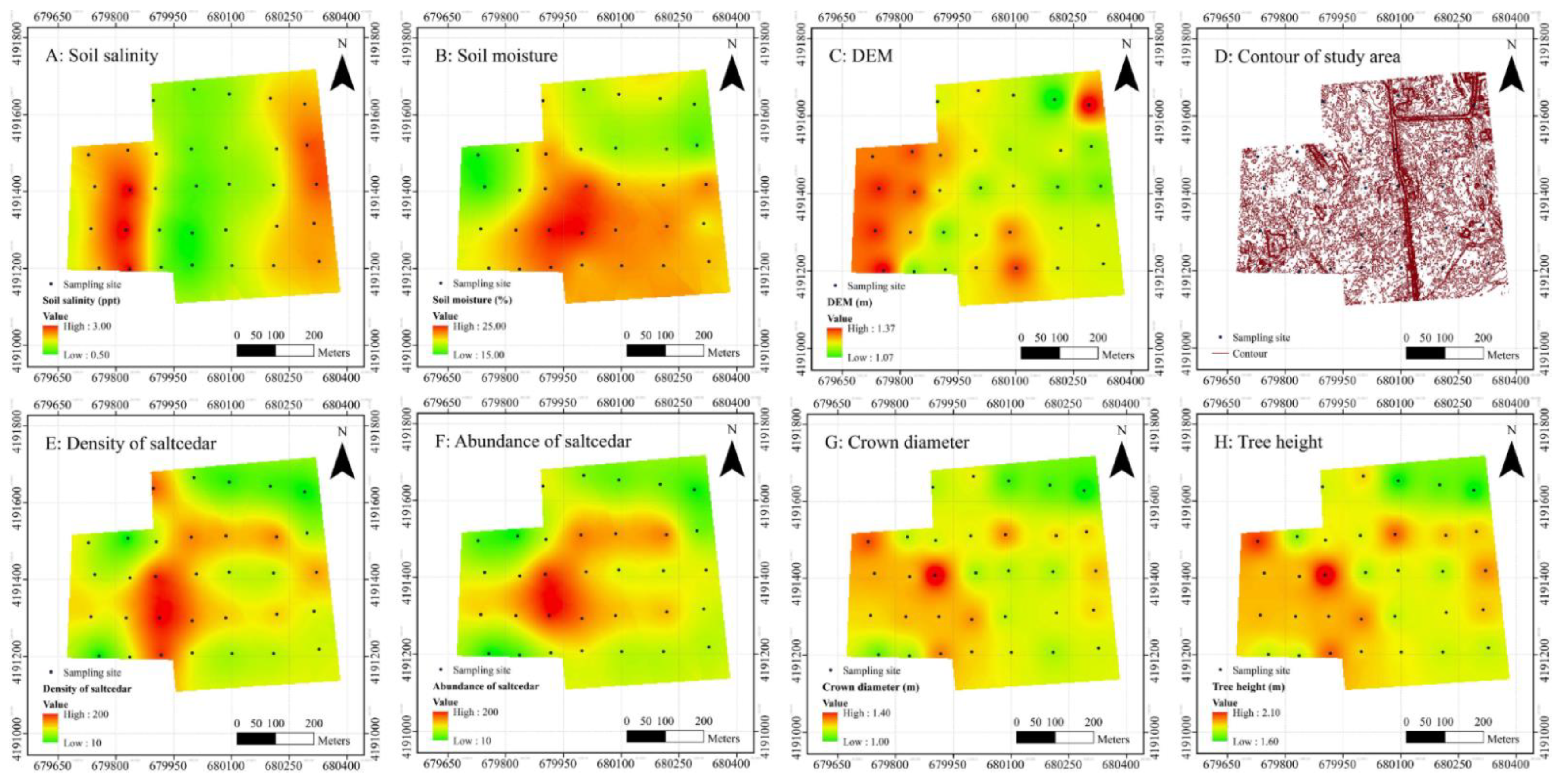
3.1. Descriptive Statistics and Spatial Distribution of Soil Properties and Saltcedar Features

3.1.1. Descriptive Statistics

The aerial survey covered an area of 33.17 ha, in which 3083 saltcedar trees were extracted through individual plant segmentation and identification with the point clouds obtained from the UAV-LiDAR system, with an average of 0.93 plants/100 m2. The spatial distributions of their tree height and crown diameter are demonstrated in Figure 2. Trees of low (<1.50 m), intermediate (1.50–2.00 m), and high (>2.00 m) height accounted for 20.82%, 50.44%, and 28.74% of all saltcedars, respectively. Trees with small (<1.00 m), intermediate (1.00–1.60 m), and large (>1.60 m) crown diameter accounted for 25.33%, 67.27%, and 7.40% of all saltcedars, respectively. For all 3083 trees, the average tree height and average crown diameter of saltcedars were 1.84 ± 0.01 m and 1.18 ± 0.01 m, respectively. Average soil salinity, average soil moisture, and average ground elevation were 1.87 ± 0.12 ppt, 21.19 ± 0.26%, and 1.23 m, respectively. Furthermore, the result of the Kolmogorov–Smirnov test showed that the original data (soil properties and saltcedar features) followed a normal distribution (p > 0.05). The coefficient of variation (CV) reflected the spatial variability of soil properties and saltcedar features. The CVs of soil salinity, density, and abundance of saltcedar (36%, 47%, and 36%, respectively) showed strong variability (CV > 30%). Maps of soil and saltcedar features based on the inverse distance weighting interpolation method also demonstrated a heterogeneous spatial distribution (Figure 3).

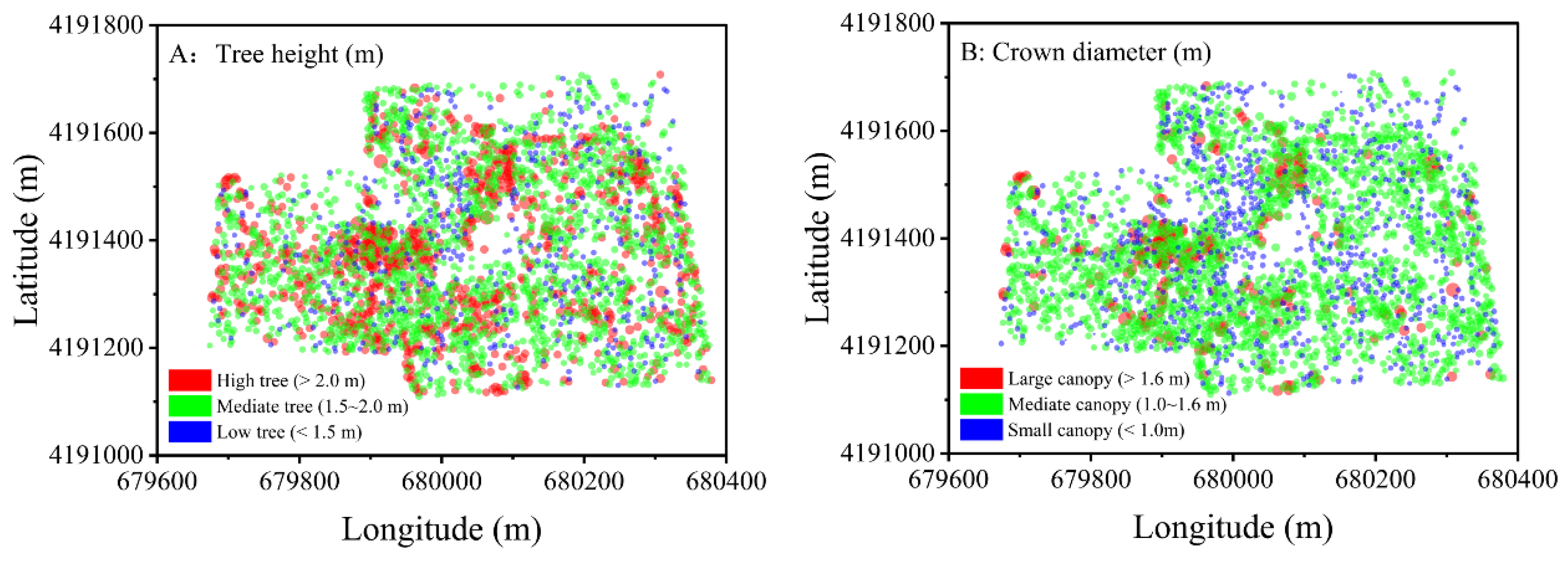
3.1.2. Spatial Distribution Patterns of Saltcedars

Second-order statistics showed that Ripley’s K function described a successive random–clustered–regular–random distribution with scale increasing. In comparison, the pair-correlation function g(r) showed a successive regular–clustered–random distribution (Figure 4). The spatial distribution pattern of the saltcedar population was clustered at a distance of 2–6 m and random above 10 m. The saltcedar population presented the strongest aggregation effect at the distance of 6 m.

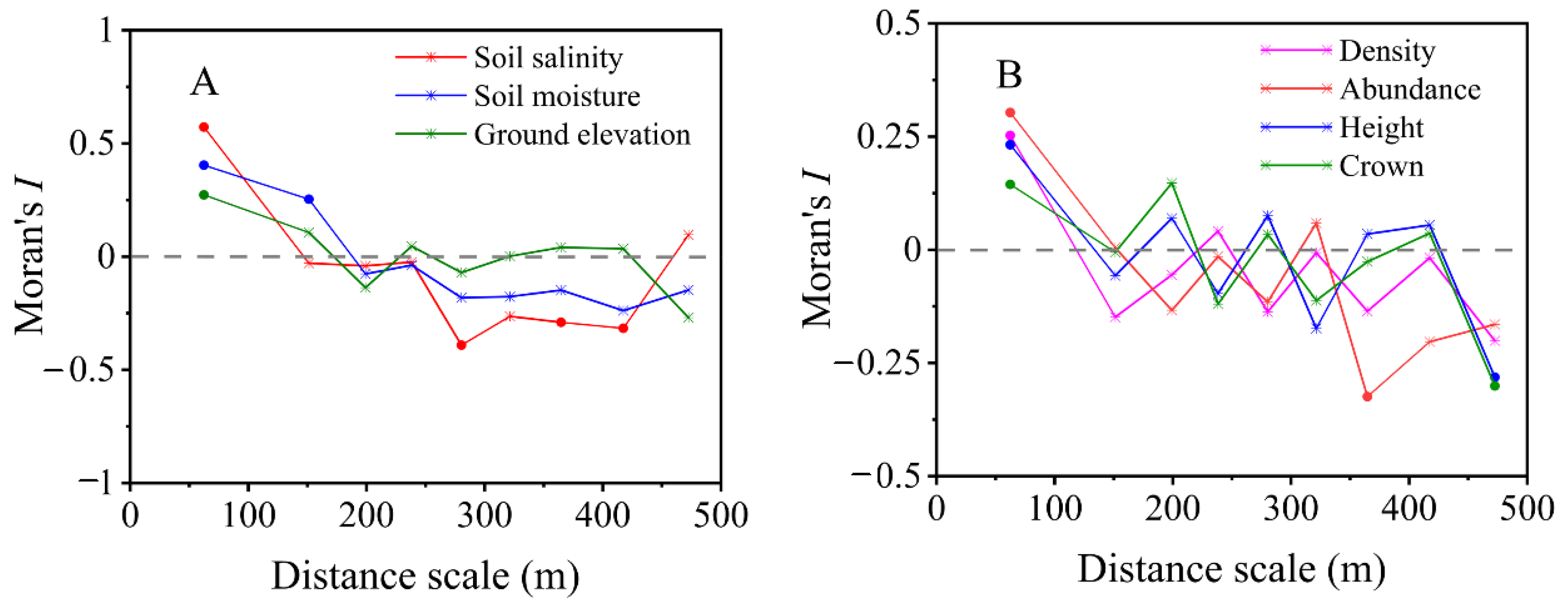
3.2. Spatial Autocorrelation Analysis of Soil and Saltcedar Variables

Both soil environmental factors and saltcedar features were significantly and positively spatially autocorrelated (Table 1). In this study, the longest boundary of the study area was 685 m and was divided into ten distance classes. The upper bound of each distance class was 125, 178, 221, 256, 305, 338, 391, 443, 502, and 685 m, successively. However, due to the large breadth of the class, the coefficients in the largest distance class were often unreliable [35]. After removing unreliable coefficients in the largest distance class, the correlograms of soil properties and saltcedar features at different distance scales showed that spatial autocorrelation decreased with the increasing distance (Figure 5). The spatial autocorrelation of elevation, soil salinity, and moisture all peaked in the 0–125 m distance class, indicating a significant positive spatial autocorrelation between closer points at 0–125 m. The spatial autocorrelation of the saltcedar population changed noticeably, especially for the abundance of saltcedar. Overall, soil properties and the saltcedar population showed a positive significant spatial autocorrelation up to 125 m.

3.3. Quantification of Factors Influencing the Distribution of Saltcedars

Stepwise regression was used to remove explanatory variables with high VIF values (>7.5) from the regression model. The OLS model between the abundance of saltcedars and explanatory variables was delineated as: YZabundance = −0.01 + 0.37 XZmoisture −0.26 XZsalinity + 0.57 XZcrown, (R2 = 0.52, p < 0.01). Using the same variables in the OLS, the environment–saltcedar relationship was also delineated through SLM and SEM (Table 2). The contribution of soil moisture and soil salinity to the abundance of saltcedar was reduced by 11.67% and 10.04% in the SLM and by 13.57% and 4.77% in the SEM, respectively. Pairs of predicted and observed values for the abundance of saltcedars in the three regression models were all discretely distributed around the 1:1 reference line (Figure 6). Spatial autocorrelation and correlograms of residuals showed no spatial autocorrelation in the residuals of OLS, SLM, and SEM (Figure 6). Thus, these models were suitable for evaluating environment–saltcedar relationships. Overall, there was no significant difference in the prediction performance of the three regression models for the abundance of saltcedar. However, comparison of the goodness of fit among three regression models indicated that R2 in SEM was greater than that in SLM and OLS. Furthermore, the AIC values of SEM were the lowest among the three regression models, in which a value of SEM differed by over three from the values in OLS and SLM (Table 2). The goodness of fit showed that, compared with OLS and SLM, SEM could better explain the variation in the abundance of saltcedars. Overall, SEM had more advantages in explaining the relationships between environmental factors and saltcedar population distribution in saltmarsh.

4. Discussion

4.1. Spatial Pattern of Saltcedar Population and Mechanisms Driving Its Formation

Our results showed that the saltcedar population exhibited an aggregated distribution at 2–6 m scales, and a random distribution at large scale (>10 m). Previous studies also reported a similar spatial distribution pattern of the saltcedar population [12,14,39,40]. The aggregation patterns of plant populations at small scales are often the result of intraspecific facilitation and local seed dispersal. Seeds of saltcedar are light and small, with hairs on the epidermis, making them highly suited to dispersal to different distances by wind or water. A previous study reported that saltcedar populations could disperse around 2.5 km yr−1 (approximately 6.85 m d−1) by wind and 11 km yr−1 (approximately 34.25 m d−1) along rivers and other waterways [41]. For wind-dispersed seeds, they usually germinate within 24 h in moist soil [42]. The intensive dispersal and germination in the short term resulted in aggregated distribution in small areas. Therefore, the aggregated distribution at 2–6 m might correspond to the distance at which the wind dispersal of seeds influenced the spatial distribution of saltcedar populations.
Biotic interaction is another important factor driving the spatial patterns of plant populations at different scales. Generally, the increasing abundance of plants at small scales promotes a balance between aboveground and underground biomass [43] or branch and leaf growth [44]. These balances contribute towards regulating the net photosynthetic and transpiration rates of plants, and benefiting their adaptation in the heterogeneous soil environments. Furthermore, the densely packed distribution of halophytes results in habitat amelioration (i.e., decline in soil salinity and increase in soil water content), enhancing seed germination and seedling growth [45,46]. As the intensity of environmental stress declines, the intraspecies facilitation weakens while intraspecific competition increases [47,48]. This phenomenon is the result of increased demand for resources by individual plants, which intensifies competition among individuals [49]. Moreover, with the increasing resistance of individual to soil environmental stresses, the interdependence among saltcedars declines. As a result of the reducing interdependence and increasing biotic competition, the plant population presents random or uniform distribution at a large scale [50]. Due to the transformation of these biological interactions, the spatial distribution pattern of the saltcedar population gradually changed from the aggregating pattern at small scales (2–6 m) to the random distribution at large scales (>10 m).

4.2. Origin of Spatial Autocorrelation in Saltcedar Population

Spatial autocorrelation is considered to be a general attribute of ecological variables and can be found at any scale in the ecosystem [24]. Spatial autocorrelation of plant populations is caused by the dependence of spatially autocorrelated environmental variables (induced or exogenous spatial autocorrelation) or by the inherent biological processes of the variable itself (inherent or endogenous spatial autocorrelation) [23,51]. In this study, results showed that soil environmental factors and saltcedar features both had positively significant spatial autocorrelation (Table 1). The saltcedar population had a positive spatial autocorrelation at distances up to 125 m (Figure 5). This indicated that saltcedar trees within a 125 m distance tended to have similar occupancy. For saltcedar populations, their spatial autocorrelation is not only caused by the spatially autocorrelated soil salinity and moisture, but also related to the ecological processes [23]. Dispersal is a major factor driving endogenous spatial autocorrelation [52]. A previous study reported that saltcedar seeds could germinate in water, even when afloat, and that seedlings could survive submerged for a few weeks [42]. Thus, the viability of the water-dispersed seeds of saltcedar could be maintained for long periods and at great distances. Even when germinating in water, seedlings could continue dispersing along rivers or other waterways until reaching suitable conditions for colonization, such as open sunny ground with low competition [42]. Therefore, the largest scale of saltcedars presenting a positively significant spatial autocorrelation (125 m) might correspond to the distance at which long-distance seed dispersal by water influenced population distributions.
The regression analysis in this study showed that the abundance of saltcedars was influenced significantly by soil salinity and moisture rather than elevation, which was consistent with previous studies [1,53]. However, only considering soil conditions could not fully explain the abundance of saltcedar. Crown diameter has a closely positive correlation with the abundance of saltcedars. This may be because the increasing crown diameter is conducive to maintaining soil moisture and providing a shading condition for the growth of seedlings, which can be regarded as intraspecific promotion [17]. These results reflected the existence of intraspecific facilitation within the saltcedar population. Moreover, it is noteworthy that the classical multiple linear regression model (OLS) in this study could not describe the environment–saltcedar relationship very well (R2 = 0.52). Two potential factors might have led to this result. One factor was that the OLS model ignored the spatial autocorrelation, which was an important factor in the spatial distribution of the saltcedar population. By comparison, SEM, which incorporated the spatial autocorrelation of saltcedars, presented a better explanatory ability in evaluating the relationship between soil environmental factors and plant spatial distribution. This was consistent with the result of other studies [25,26,31,54]. Another factor might be due to the accuracy of individual plant segmentation and identification. In this research, different vegetation types were separated based on tree height. Some young trees with low height might have been ignored or classified into other types. This might also have resulted in the unsatisfactory correlation coefficient. In the future, an aerial survey of vegetation types, and a combination of a UAV-LiDAR system with multispectral imaging technology or simultaneous localization and mapping (SLAM) technology, would promote the quality of point clouds and the accuracy of individual plant segmentation and identification [55]. Other effective measures include increasing the density of fixed monitoring sites, prolonging the monitoring time, and enriching the monitoring soil elements.
Overall, as a result of intraspecific facilitation and seed dispersal, the saltcedar population was aggregated at 2–6 m scales and presented a positive spatial autocorrelation at distances up to 125 m. The existence of positive spatial autocorrelation in the saltcedar population led to overestimation of environmental factors when analyzing the environment–saltcedar relationship by the traditional OLS method. This study highlighted the importance of spatial autocorrelation when analyzing the environment–saltcedar relationships. Future study should cautiously estimate the influence of soil environmental factors on the spatial distribution of saltcedar populations.

4.3. Implications for Ecological Management and Restoration of Saltcedar Population

Currently, saltcedar populations, as well as other halophytes in coastal saltmarsh, are undergoing increasingly serious degradation and fragmentation because of the multiple impacts of global climate change and human disturbance [4,5]. Generally, spatial pattern analysis plays an instructional role for the restoration and management of plant populations. Based on life history strategies and distribution patterns of species, different implementation approaches are adopted for population restoration. Previous studies suggest that restoration efforts would be more effective for trees in forests and corals with an r-selected life history if organisms were added to landscapes in uniform and gridded patterns [56,57]. Conversely, for the plants with a competitive disadvantage or inhabiting harsh environments, aggregated arrangement could be more effective in increasing flowering individuals and reproductive biomass, which would contribute to maintaining the plant population in the following generations [58].
In this study, the results suggested an aggregation distribution of the saltcedar population at small scales and a positive significant relationship between the abundance and crown diameter of saltcedars. Consistent with previous studies, these results implied that saltcedar individuals could be transplanted as patches with scopes of 2–6 m. Aggregation of saltcedar individuals would promote the survival rates and colonization ability after transplantation into a new habitat [39]. Some engineering measures in favor of hydrological connectivity are also recommended to restore the saltcedar population through assisting seed dispersal. For example, ditch excavation provides channels for seed spreading with water [59]. Modifying microtopography contributes to seed interception and provides a surface runoff channel for seed dispersal [60,61].
In addition, the UAV-LiDAR system shows good application prospects in topographic mapping, plant population monitoring, and pattern analysis in saltmarsh. As an emerging remote sensing technology, the UAV-LiDAR system allows the efficient survey of target areas at different spatial scales, especially local-scale monitoring [62]. UAV-LiDAR systems overcome the disadvantages of traditional remote sensing approaches, which are not able to meet the time frequency requirements in analyzing ecological processes and the required high spatial resolution in analyzing fine-scale information [63]. Future research on the spatial pattern analysis and restoration of plant populations in saltmarsh should be conducted over the long term and at broad scales, combining UAV-LiDAR systems with diverse monitoring methods, such as remote sensing technologies and multispectral or hyperspectral imaging techniques. Such information would assist in understanding the distribution patterns of plant populations at different spatiotemporal scales and guide theoretically their ecological management and restoration in saltmarsh.

5. Conclusions

This study extracted plant and soil parameters by integrating the UAV-LiDAR system with fixed soil environment measurements, and further analyzed the spatial pattern of the saltcedar population and the environment–saltcedar relationship, incorporating the fine-scale spatial autocorrelation. The results showed that saltcedars presented clustered distribution at small scales (2–6 m) due to intraspecific facilitation and wind dispersal of seeds. In comparison, intraspecific competition was responsible for the random distribution of saltcedars at large scale (>10 m). The saltcedar population had a positive significant spatial autocorrelation, with Moran’s I peaking at 0–125 m, which was related to water-dispersed seeds. After incorporating the spatial autocorrelation of saltcedars when analyzing the environment–saltcedar relationship, the interpretation ability of soil moisture and salinity for the abundance of saltcedars decreased by 11.67% and 10.04% in SLM, and by 13.57% and 4.77% in SEM, respectively. Meanwhile, there was a significant positive correlation between the abundance and crown diameter of saltcedars, which had a stronger effect on the abundance of saltcedar (>55%) than soil factors.
Consequently, these results suggested that due to intraspecific facilitation and seed dispersal, the saltcedar population was clustered and autocorrelated spatially at different scales. This spatial pattern improved the adaptability of saltcedars to environmental stress and thus reduced the impact of environmental factors on the abundance of saltcedar. Therefore, during the restoration of the saltcedar population in the future, biotic interactions and seed dispersal should be given more attention, in addition to the existing measures (e.g., improving environmental factors). Transplanting saltcedars as patches with appropriate size and constructing channels to facilitate seed dispersal are both recommended measures to restore and manage the saltcedar population in saltmarsh. These measures will profit the restoration and management of the saltcedar population as well as other halophytes in coastal saltmarsh.

Author Contributions

Conceptualization, L.J. and T.S.; Data curation, L.J. and T.S.; Formal analysis, L.J., T.S. and P.Z.; Funding acquisition, T.S.; Investigation, L.J. and Y.Z.; Methodology, L.J., Y.Z. and P.Z.; Project administration, T.S.; Resources, T.S.; Software, L.J. and Y.Z.; Supervision, T.S.; Validation, T.S.; Visualization, L.J.; Writing—original draft, L.J.; Writing—review and editing, T.S., W.Y., D.S. and Q.L. All authors have read and agreed to the published version of the manuscript.

Funding

This work was supported by the Joint Funds of the National Natural Science Foundation of China (No. U1806217) and the Fund for Innovative Research Group of the National Natural Science Foundation of China (No. 51721093).

Institutional Review Board Statement

Not applicable.

Informed Consent Statement

Not applicable.

Data Availability Statement

Not applicable.

Acknowledgments

We sincerely thank Qingchen Li and Yao Lu (South Surveying & Mapping Instrument Co., Ltd.) and Qiang Tan (Beijing SureStar Technology Co. Ltd.) for their technical support in point cloud collection and processing.

Conflicts of Interest

The authors declare that they have no known competing financial interests or personal relationships that could have appeared to influence the work reported in this paper.

References

  1. Gao, M.; Wang, X.; Hui, C.; Yi, H.; Zhang, C.; Wu, X.; Bi, X.; Wang, Y.; Xiao, L.; Wang, D. Assembly of plant communities in coastal wetlands-the role of saltcedar Tamarix chinensis during early succession. J. Plant Ecol. 2015, 8, 539–548. [Google Scholar] [CrossRef] [Green Version]
  2. Qi, M.; Sun, T.; Zhan, M.; Xue, S. Simulating dynamic vegetation changes in a tidal restriction area with relative stress tolerance curves. Wetlands 2015, 36, 31–43. [Google Scholar] [CrossRef]
  3. Feng, Y.; Sun, T.; Zhu, M.; Qi, M.; Yang, W.; Shao, D. Salt marsh vegetation distribution patterns along groundwater table and salinity gradients in yellow river estuary under the influence of land reclamation. Ecol. Indic. 2018, 92, 82–90. [Google Scholar] [CrossRef]
  4. Cui, B.; Yang, Q.; Zhang, K.; Zhao, X.; You, Z. Responses of saltcedar (Tamarix chinensis) to water table depth and soil salinity in the Yellow River Delta, China. Plant Ecol. 2010, 209, 279–290. [Google Scholar] [CrossRef]
  5. Liu, Q.; Li, F.; Zhang, Q.; Li, J.; Zhang, Y.; Tu, C.; Ouyang, Z. Impact of water diversion on the hydrogeochemical characterization of surface water and groundwater in the Yellow River Delta. Appl. Geochem. 2014, 48, 83–92. [Google Scholar] [CrossRef]
  6. Sun, Q.; Lin, H.; Zhang, M.; Jiao, L.; Zhang, Y.; Yang, W.; Sun, T. Research progress on ecological restoration of coastal salt marsh. J. Beijing Norm. Univ. 2021, 57, 151–158. [Google Scholar]
  7. Jiao, L.; Li, F.; Liu, X.; Wang, S.; Zhou, Y. Fine-scale distribution patterns of Phragmites australis populations across an environmental gradient in the salt marsh wetland of Dunhuang, China. Sustainability 2020, 12, 1671. [Google Scholar] [CrossRef] [Green Version]
  8. Fullerton, A.H.; Steel, E.A.; Lange, I.; Caras, Y. Effects of spatial pattern and economic uncertainties on freshwater habitat restoration planning: A simulation exercise. Restor. Ecol. 2010, 18, 354–369. [Google Scholar] [CrossRef] [Green Version]
  9. Larson, A.J.; Churchill, D. Tree spatial patterns in fire-frequent forests of western North America, including mechanisms of pattern formation and implications for designing fuel reduction and restoration treatments. For. Ecol. Manag. 2012, 267, 74–92. [Google Scholar] [CrossRef]
  10. Viers, J.H.; Fremier, A.K.; Hutchinson, R.A.; Quinn, J.F.; Thorne, J.H.; Vaghti, M.G. Multiscale patterns of riparian plant diversity and implications for restoration. Restor. Ecol. 2012, 20, 160–169. [Google Scholar] [CrossRef]
  11. Wu, P.; Peng, X.; Yang, S.; Gao, Y.; Bai, F.; Yi, S.; Du, N.; Guo, W. Spatial distribution patterns and correlation of Tamarix chinensis population in coastal wetlands of Shandong, China. Chin. J. Plant Ecol. 2019, 43, 817–824. [Google Scholar]
  12. Liu, Y.; Liu, J.; Chen, Y.; Jing, S.; Feng, R.; Mao, G. Research on distribution patterns and population structure of Tamarix chinensis in the intertidal zone of coastal wetlands in Yellow River Delta. Ecol. Sci. 2017, 36, 153–158. [Google Scholar]
  13. Zhao, X.; Cui, B.; Sun, T.; Lv, J.; Lu, F. Analysis of spatial point pattern of Tamarix chinensis in different habitats. Ecol. Sci. 2011, 30, 142–148. [Google Scholar]
  14. He, Q.; Cui, B.; Hu, Q.; Yang, S.; Zhao, X. Fractal analysis on the distribution patterns of Tamarix chinensis under environmental gradients of different water table depth. Bull. Soil Water Conser. 2008, 28, 70–73. [Google Scholar]
  15. Chambers, L.G.; Osborne, T.Z.; Reddy, K.R. Effect of salinity-altering pulsing events on soil organic carbon loss along an intertidal wetland gradient: A laboratory experiment. Biogeochemistry 2013, 115, 363–383. [Google Scholar] [CrossRef]
  16. Bertness, M.D.; Callaway, R. Positive interactions in communities. Trends Ecol. Evol. 1994, 9, 191–193. [Google Scholar] [CrossRef]
  17. Bertness, M.D.; Hacker, S.D. Physical stress and positive associations among marsh plants. Am. Nat. 1994, 144, 363–372. [Google Scholar] [CrossRef]
  18. Legendre, P.; Dale, M.R.T.; Fortin, M.J.; Gurevitch, J.; Hohn, M.; Myers, D. The consequences of spatial structure for the design and analysis of ecological field surveys. Ecography 2002, 25, 601–615. [Google Scholar] [CrossRef] [Green Version]
  19. Valcu, M.; Kempenaers, B. Spatial autocorrelation: An overlooked concept in behavioral ecology. Behav. Ecol. 2010, 21, 902–905. [Google Scholar] [CrossRef] [PubMed] [Green Version]
  20. Kissling, W.D.; Carl, G. Spatial autocorrelation and the selection of simultaneous autoregressive models. Glob. Ecol. Biogeogr. 2008, 17, 59–71. [Google Scholar] [CrossRef]
  21. Kim, D. Modeling spatial and temporal dynamics of plant species richness across tidal creeks in a temperate salt marsh. Ecol. Indic. 2018, 93, 188–195. [Google Scholar] [CrossRef]
  22. Maheu-Giroux, M.; de Blois, S. Landscape ecology of Phragmites australis invasion in networks of linear wetlands. Landscape Ecol. 2006, 22, 285–301. [Google Scholar] [CrossRef]
  23. Badenhausser, I.; Gouat, M.; Goarant, A.; Cornulier, T.; Bretagnolle, V. Spatial autocorrelation in farmland grasshopper assemblages (Orthoptera: Acrididae) in western France. Environ. Entomol. 2012, 41, 1050–1061. [Google Scholar] [CrossRef] [PubMed]
  24. Legendre, P. Spatial autocorrelation: Trouble or new paradigm? Ecology 1993, 74, 1659–1673. [Google Scholar] [CrossRef]
  25. Zhang, L.; Ma, Z.; Guo, L. An evaluation of spatial autocorrelation and heterogeneity in the residuals of six regression models. For. Sci. 2009, 55, 533–548. [Google Scholar]
  26. Marrot, P.; Garant, D.; Charmantier, A.; Hadfield, J. Spatial autocorrelation in fitness affects the estimation of natural selection in the wild. Methods Ecol. Evol. 2015, 6, 1474–1483. [Google Scholar] [CrossRef] [Green Version]
  27. Wiegand, T.; Moloney, K.A. Rings, circles, and null-models for point pattern analysis in ecology. Oikos 2004, 104, 209–229. [Google Scholar] [CrossRef]
  28. Soberón, J. Grinnellian and Eltonian niches and geographic distributions of species. Ecol. Lett. 2007, 10, 1115–1123. [Google Scholar] [CrossRef] [PubMed]
  29. Kneitel, J.M.; Chase, J.M. Trade-offs in community ecology: Linking spatial scales and species coexistence. Ecol. Lett. 2004, 7, 69–80. [Google Scholar] [CrossRef] [Green Version]
  30. Meng, Q.; Cieszewski, C.J.; Strub, M.R.; Borders, B.E. Spatial regression modeling of tree height–diameter relationships. Can. J. For. Res. 2009, 39, 2283–2293. [Google Scholar] [CrossRef]
  31. Wang, Q.; Ni, J.; Tenhunen, J. Application of a geographically-weighted regression analysis to estimate net primary production of Chinese forest ecosystems. Glob. Ecol. Biogeogr. 2005, 14, 379–393. [Google Scholar] [CrossRef]
  32. Kim, D.; Shin, Y.H. Spatial autocorrelation potentially indicates the degree of changes in the predictive power of environmental factors for plant diversity. Ecol. Indic. 2016, 60, 1130–1141. [Google Scholar] [CrossRef]
  33. Lichstein, J.W.; Simons, T.R.; Shriner, S.A.; Franzreb, K.E. Spatial autocorrelation and autoregressive models in ecology. Ecol. Monogr. 2002, 72, 445–463. [Google Scholar] [CrossRef]
  34. Wiegand, T.; Moloney, K.A. Handbook of Spatial Point-Pattern Analysis in Ecology; Chapman and Hall/CRC: New York, NY, USA, 2014. [Google Scholar]
  35. Rosenberg, M.S. The bearing correlogram: A new method of analyzing directional spatial autocorrelation. Geogr. Anal. 2000, 32, 267–278. [Google Scholar] [CrossRef]
  36. Dale, M.R.T.; Fortin, M.J. Spatial Analysis: A Guide for Ecologists; Cambridge University Press: Cambridge, UK, 2005. [Google Scholar]
  37. Rosenberg, M.S.; Anderson, C.D. PASSaGE: Pattern Analysis, Spatial Statistics and Geographic Exegesis. Version 2. Methods Ecol. Evol. 2011, 2, 229–232. [Google Scholar] [CrossRef]
  38. Ding, J.; Zhao, W.; Fu, B.; Wang, S.; Fan, H. Variability of Tamarix spp. characteristics in riparian plant communities are affected by soil properties and accessibility of anthropogenic disturbance in the lower reaches of Heihe River, China. For. Ecol. Manag. 2018, 410, 174–186. [Google Scholar] [CrossRef]
  39. Zhao, X.; Lv, J.; Sun, T. Relations between the distribution of vegetation and environment in the Yellow River Delta and SPPA for Chinese tamarisk spatial distribution. J. Beijing For. Univ. 2009, 31, 29–36. [Google Scholar]
  40. Wu, Y.; Dai, L.; Wang, Y.; Xie, L.; Zhao, S.; Liu, Y.; Zhang, M.; Zhang, Z. Coexistence mechanisms of Tamarix chinensis and Suaeda salsa in the Yellow River Delta, China. Environ. Sci. Pollut. Res. 2020, 27, 26172–26181. [Google Scholar] [CrossRef]
  41. Pearce, C.M.; Smith, D.G. Saltcedar: Distribution, abundance, and dispersal mechanisms, northern Montana, USA. Wetlands 2003, 23, 215–228. [Google Scholar] [CrossRef]
  42. Di Tomaso, J.M. Impact, biology, and ecology of saltcedar (Tamarix spp.) in the southwestern United States. Weed Technol. 1998, 12, 326–336. [Google Scholar] [CrossRef]
  43. Weiner, J. Allocation, plasticity and allometry in plants. Perspect. Plant Ecol. Evol. Syst. 2004, 6, 207–215. [Google Scholar] [CrossRef]
  44. Westoby, M.; Falster, D.S.; Moles, A.T.; Vesk, P.A.; Wright, I.J. Plant ecological strategies: Some leading dimensions of variation between species. Annu. Rev. Ecol. Syst. 2002, 33, 125–159. [Google Scholar] [CrossRef] [Green Version]
  45. Reijers, V.C.; van den Akker, M.; Cruijsen, P.M.J.M.; Lamers, L.P.M.; van der Heide, T. Intraspecific facilitation explains the persistence of Phragmites australis in modified coastal wetlands. Ecosphere 2019, 10, e02842. [Google Scholar] [CrossRef] [Green Version]
  46. Cao, Q.; Yang, B.; Li, J.; Wang, R.; Liu, T.; Xiao, H. Characteristics of soil water and salt associated with Tamarix ramosissima communities during normal and dry periods in a semi-arid saline environment. Catena 2020, 193, 104661. [Google Scholar] [CrossRef]
  47. Brooker, R.W.; Maestre, F.T.; Callaway, R.M.; Lortie, C.L.; Cavieres, L.A.; Kunstler, G.; Liancourt, P.; Tielbörger, K.; Travis, J.M.J.; Anthelme, F.; et al. Facilitation in plant communities: The past, the present, and the future. J. Ecol. 2007, 96, 18–34. [Google Scholar] [CrossRef] [Green Version]
  48. Qi, M.; Sun, T.; Xue, S.; Yang, W.; Shao, D.; Martínez-López, J. Competitive ability, stress tolerance and plant interactions along stress gradients. Ecology 2018, 99, 848–857. [Google Scholar] [CrossRef] [PubMed]
  49. Lin, Y.; Berger, U.; Yue, M.; Grimm, V. Asymmetric facilitation can reduce size inequality in plant populations resulting in delayed density-dependent mortality. Oikos 2016, 125, 1153–1161. [Google Scholar] [CrossRef]
  50. Yang, J.; Zhang, Z.; Dawazhaxi; Wang, B.; Li, Q.; Yu, Q.; Ou, X.; Ali, K. Spatial distribution patterns and intra-specific competition of pine (Pinus yunnanensis) in abandoned farmland under the Sloping Land Conservation Program. Ecol. Eng. 2019, 135, 17–27. [Google Scholar] [CrossRef]
  51. Wagner, H.H.; Fortin, M.J. Spatial analysis of landscapes: Concepts and statistics. Ecology 2005, 86, 1975–1987. [Google Scholar] [CrossRef] [Green Version]
  52. Beale, C.M.; Lennon, J.J.; Yearsley, J.M.; Brewer, M.J.; Elston, D.A. Regression analysis of spatial data. Ecol. Lett. 2010, 13, 246–264. [Google Scholar] [CrossRef]
  53. Terrones, A.; Moreno, J.; Agulló, J.C.; Villar, J.L.; Vicente, A.; Alonso, M.Á.; Juan, A. Influence of salinity and storage on germination of Tamarix taxa with contrasted ecological requirements. J. Arid Environ. 2016, 135, 17–21. [Google Scholar] [CrossRef]
  54. Overmars, K.P.; de Koning, G.H.J.; Veldkamp, A. Spatial autocorrelation in multi-scale land use models. Ecol. Model. 2003, 164, 257–270. [Google Scholar] [CrossRef]
  55. He, G.; Yuan, X.; Zhuang, Y.; Hu, H. An Integrated GNSS/LiDAR-SLAM pose estimation framework for large-scale map building in partially GNSS-denied environments. IEEE T. Instrum. Meas. 2021, 70, 1–9. [Google Scholar]
  56. Sleeman, J.C.; Boggs, G.S.; Radford, B.C.; Kendrick, G.A. Using agent-based models to aid reef restoration: Enhancing coral cover and topographic complexity through the spatial arrangement of coral transplants. Restor. Ecol. 2005, 13, 685–694. [Google Scholar] [CrossRef]
  57. Pringle, R.M.; Doak, D.F.; Brody, A.K.; Jocque, R.; Palmer, T.M. Spatial pattern enhances ecosystem functioning in an African savanna. PLoS Biol. 2010, 8, e1000377. [Google Scholar] [CrossRef]
  58. Stoll, P.; Prati, D. Intraspecific aggregation alters competitive interactions in experimental plant communities. Ecology 2001, 82, 319–327. [Google Scholar] [CrossRef]
  59. Zeng, S.; Zhang, T.; Gao, Y.; Li, B.; Fang, C.; Flory, S.L.; Zhao, B. Road effects on vegetation composition in a saline environment. J. Plant Ecol. 2012, 5, 206–218. [Google Scholar] [CrossRef] [Green Version]
  60. Wang, Q.; Cui, B.; Luo, M.; Qiu, D.; Shi, W.; Xie, C. Microtopographic structures facilitate plant recruitment across a saltmarsh tidal gradient. Aquat. Conserv. Mar. Freshwat. Ecosyst. 2019, 29, 1336–1346. [Google Scholar] [CrossRef]
  61. Wang, Q.; Cui, B.; Luo, M.; Shi, W. Designing microtopographic structures to facilitate seedling recruitment in degraded salt marshes. Ecol. Eng. 2018, 120, 266–273. [Google Scholar] [CrossRef]
  62. Zhang, J.; Hu, J.; Lian, J.; Fan, Z.; Ouyang, X.; Ye, W. Seeing the forest from drones: Testing the potential of lightweight drones as a tool for long-term forest monitoring. Biol. Conserv. 2016, 198, 60–69. [Google Scholar] [CrossRef]
  63. Anderson, K.; Gaston, K.J. Lightweight unmanned aerial vehicles will revolutionize spatial ecology. Front. Ecol. Environ. 2013, 11, 138–146. [Google Scholar] [CrossRef] [Green Version]
Figure 1. Site location and DOM of the study area in the Yellow River Delta, China.
Sustainability 13 08291 g001
Figure 2. Spatial distribution of all saltcedar (Tamarix chinensis) trees with different tree heights (A) and different crown diameters (B) in the study area.
Sustainability 13 08291 g002
Figure 3. Maps of soil properties (AD) and saltcedar (Tamarix chinensis) features (EH) based on inverse distance weighting interpolation.
Sustainability 13 08291 g003
Figure 4. Univariate point pattern analyses of the spatial distribution of saltcedar (Tamarix chinensis) based on Ripley’s K function (A) and pair-correlation functions g(r) under a heterogeneous Poisson null model (B). The simulation envelopes (grey interval) correspond to the 5% and 95% confidence intervals. The insert figures describe the point pattern analysis of saltcedars at the maximum distance (400 m).
Sustainability 13 08291 g004
Figure 5. Nondirectional spatial correlogram on the features of (A) soil and (B) saltcedar (Tamarix chinensis). Solid circles were significant at p < 0.05, while asterisks were nonsignificant. The upper bound of each distance class was 125, 178, 221, 256, 305, 338, 391, 443, and 502 m, successively. The coefficient in the largest distance class was often unreliable, due to the large breadth of the class and/or paucity of relevant pairs of points (depending on how the classes were designed); thus, this value was often not plotted in correlogram analyses [35]. All correlograms were globally significant (p < 0.05).
Sustainability 13 08291 g005
Figure 6. Performance of different regression models. Scatter diagrams between observed and predicted values of the abundance of saltcedars (Tamarix chinensis) are shown in the upper three panels (A: OLS; B: SLM; C: SEM). Nondirectional spatial correlograms for the residuals of different regression models are shown in the bottom three panels (D: OLS; E: SLM; F: SEM). Solid circles indicate the significant spatial autocorrelation (p < 0.05) and asterisks indicate the nonsignificant spatial autocorrelation. All correlograms were globally significant (p < 0.05).
Sustainability 13 08291 g006
Table 1. Moran’s I and significant test of the features of soil and saltcedar (Tamarix chinensis) in the study area.
Moran’s IZscorep
Soil salinity0.504.82p < 0.05
Soil moisture0.424.00p < 0.05
Ground elevation0.233.40p < 0.05
Density0.192.26p < 0.05
Abundance0.262.61p < 0.05
Crown diameter0.272.76p < 0.05
Tree height0.2016.78p < 0.05
Table 2. Parameter estimation and goodness of fit test of OLS, SLM, and SEM.
VariableCoefficientSEt-StatisticProbability
OLSConstant−0.010.120.000.98
Zmoisture0.370.132.870.00 **
Zsalinity−0.260.13−2.020.04 *
Zcrown0.570.124.640.00 **
Goodness of fitR2 = 0.52, LIK = −32.36, AIC = 76.95, SC = 78.71
SLMConstant0.040.110.380.71
Zmoisture0.410.133.170.00 **
Zsalinity−0.290.12−2.390.02 *
Zcrown0.570.114.990.00 **
ρ−0.230.24−0.940.35
Goodness of fitR2 = 0.58, LIK = −32.10, AIC = 74.21, SC = 81.69
SEMConstant0.020.100.160.87
Zmoisture0.360.113.140.00 **
Zsalinity−0.270.11−2.390.02 *
Zcrown0.550.114.860.00 **
λ−0.140.30−0.450.65
Goodness of fitR2 = 0.57, LIK = −32.01, AIC = 72.61, SC = 78.60
*: indicates a statistically significant coefficient (p < 0.05); **: indicates a statistically significant coefficient (p < 0.01).
Publisher’s Note: MDPI stays neutral with regard to jurisdictional claims in published maps and institutional affiliations.

