
Recommended System for Cluster Head Selection in a Remote Sensor Cloud Environment Using the Fuzzy-Based Multi-Criteria Decision-Making Technique

 ,
, 
 and
and
Abstract
:1. Introduction
2. Related Work
3. Proposed Work
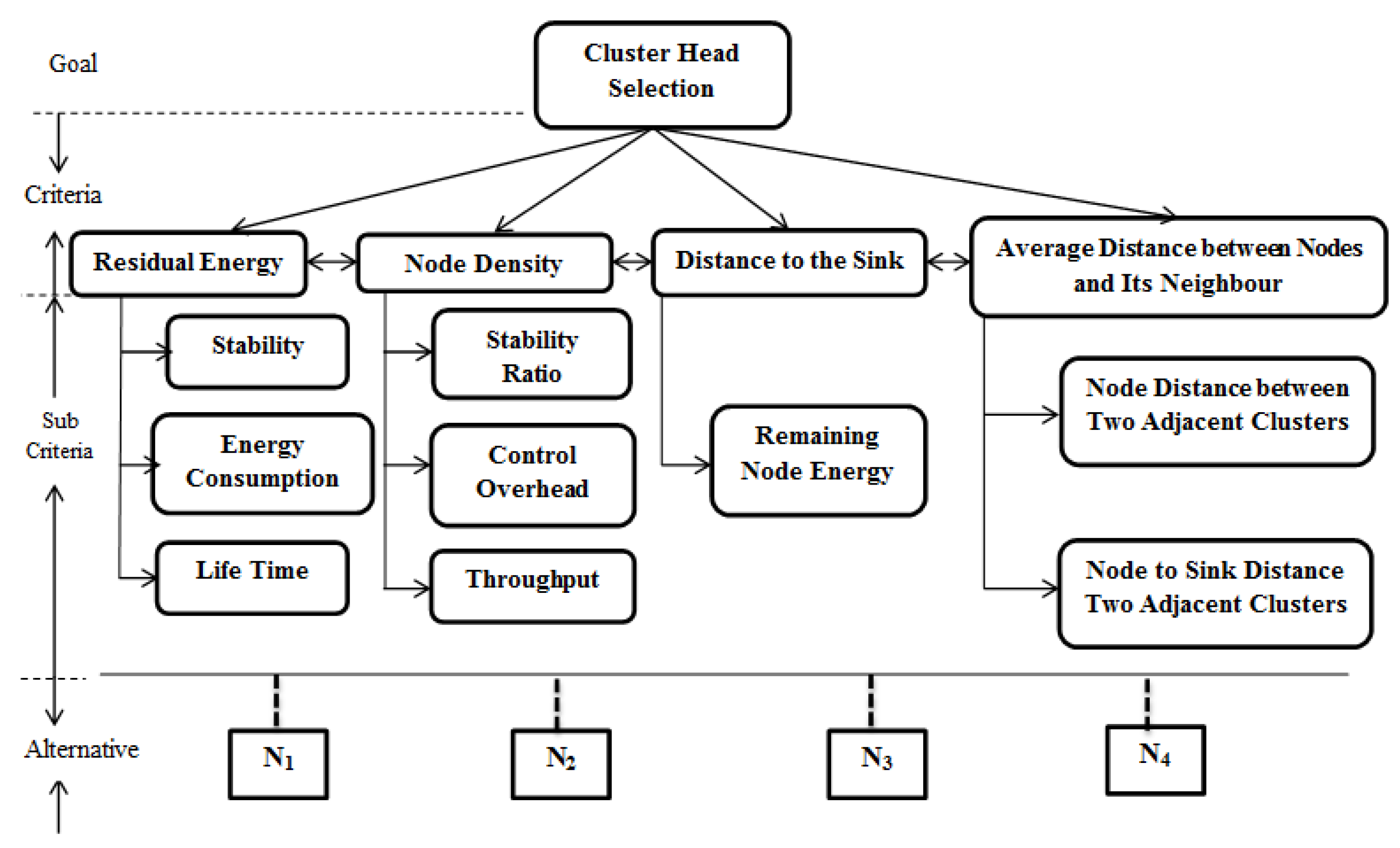
3.1. Cluster Head Selection Using Fuzzy MCDM Techniques
3.2. CH Selection Fuzzy AHP Modes
3.3. Determining the Weights of Sub-Criteria and Alternatives with Respect to the Criteria
3.4. CH Selection Fuzzy ANP Mode
3.5. Determining the Weights of Sub-Criteria and Alternatives with Respect to the Criteria
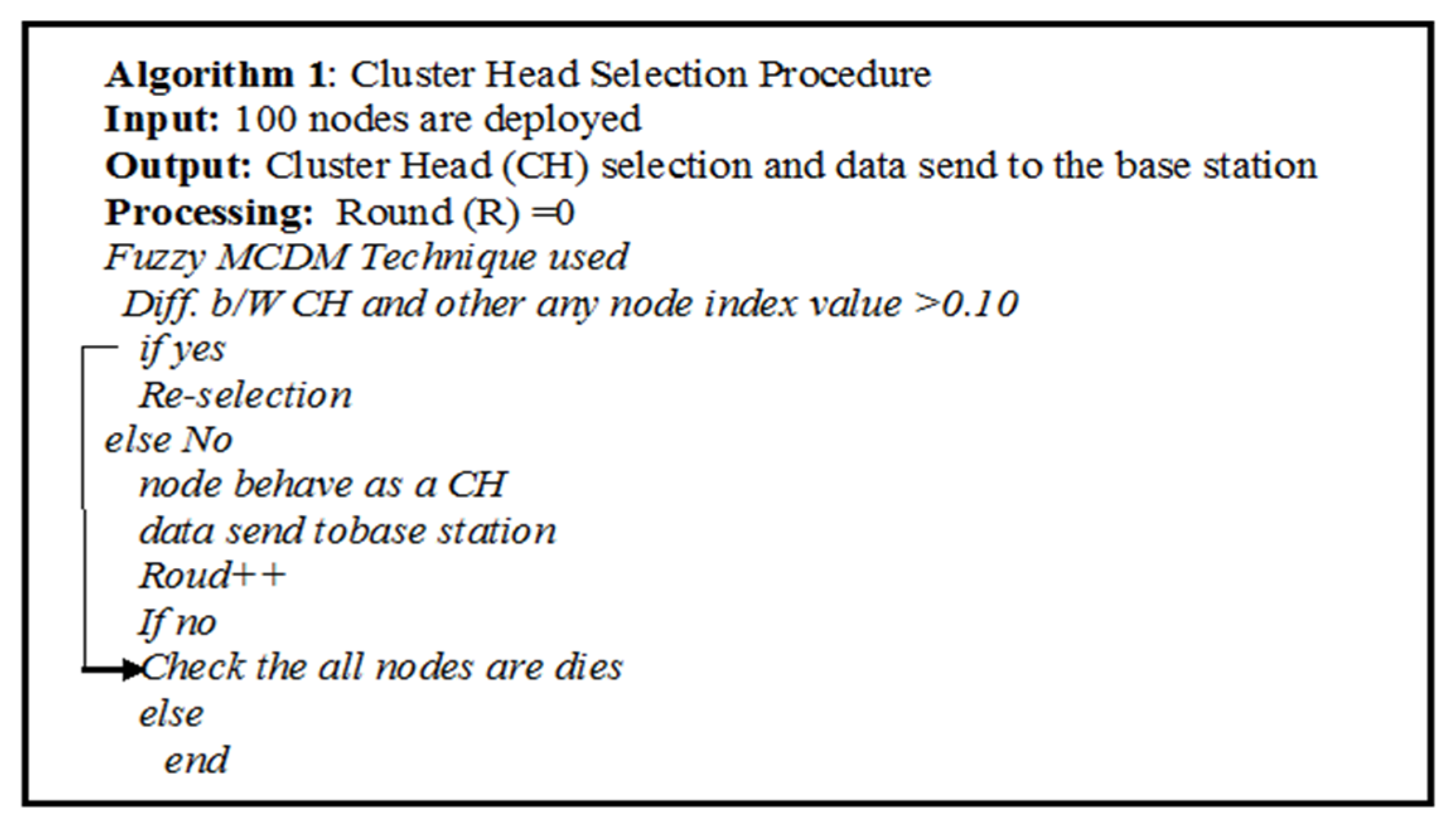
3.6. Proposed Algorithm
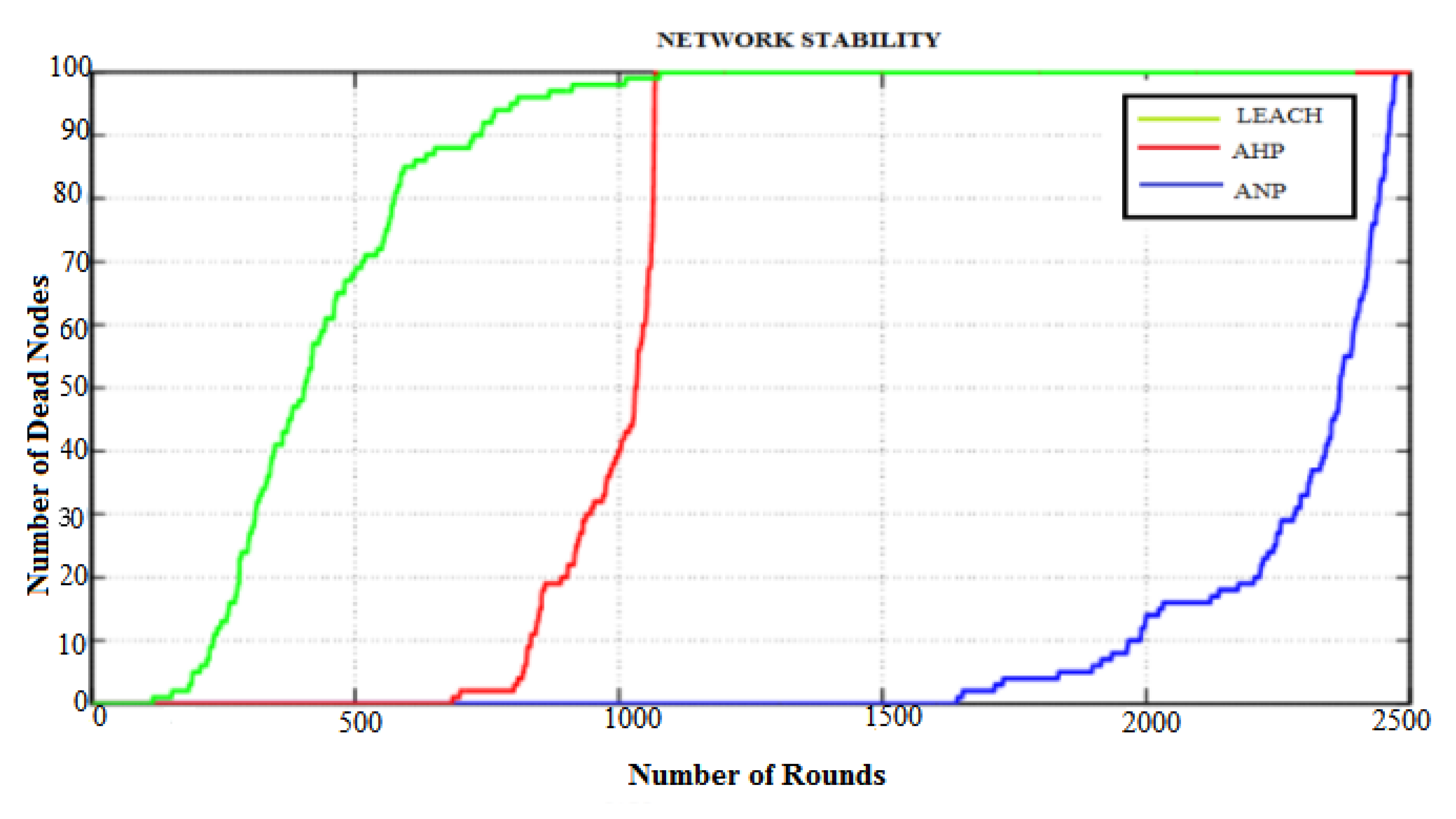
4. Experiments and Evaluation
5. Conclusions
Author Contributions
Funding
Institutional Review Board Statement
Informed Consent Statement
Data Availability Statement
Acknowledgments
Conflicts of Interest
References
- Dash, S.K.; Mohapatra, S.; Pattnaik, P.K. Survey on Application of Wireless Sensor Network Using Cloud Computing. Int. J. Comput. Sci. Emerg. Technol. 2010, 1, 50–55. [Google Scholar]
- Nimbits Data Logging Cloud Sever. Available online: http://www.nimbits.com (accessed on 5 March 2021).
- Pachube Feed Cloud Service. Available online: http://www.pachube.com (accessed on 3 January 2021).
- Kurata, N.; Suzuki, M.; Saruwatari, S.; Morikawa, H. Actual application of ubiquitous structural monitoring system using wireless sensor networks. In Proceedings of the 14th World Conference on Earthquake Engineering (WCEE’08), Beijing, China, 12–17 October 2008. [Google Scholar]
- Lan, K.T. What’s Next? Sensor+Cloud? In Proceeding of the 7th International Workshop on Data Management for Sensor Networks, Seattle, WA, USA, 29 August 2010; ACM Digital Library: New York, NY, USA, 2010; pp. 971–978. [Google Scholar]
- Google Health. Available online: http://www.google.com/health (accessed on 17 April 2021).
- Korea u-Life Care System. Available online: http://www.apan.net/meetings/HongKong2011/Session/Agriculture.php/ (accessed on 3 December 2020).
- Kim, K.; Lee, S.; Yoo, H.; Kim, D. Agriculture Sensor-Cloud Infrastructure and Routing Protocol in the Physical Sensor Network Layer. Int. J. Distrib. Sens. Netw. 2014, 10, 1–13. [Google Scholar] [CrossRef]
- Yuriyama, M.; Kushida, T.; Itakura, M. A new model of accelerating service innovation with sensor-cloud infrastructure. In Proceedings of the Annual SRII Global Conference (SRII’11), San Jose, CA, USA, 29 March–2 April 2011; pp. 308–314. [Google Scholar]
- Liu, H.-C.; Yang, M.; Zhou, M.; Tian, G. An Integrated Multi-Criteria Decision Making Approach to Location Planning of Electric Vehicle Charging Stations. IEEE Trans. Intell. Transp. Syst. 2018, 20, 362–373. [Google Scholar] [CrossRef]
- Dash, S.K.; Sahoo, J.P.; Mohapatra, S.; Pati, S.P. Sensor-cloud: Assimilation of wireless sensor network and the cloud. In Advances in Computer Science and Information Technology. Networks and Communications, Proceedings of the Second International Conference, Bangalore, India, 2–4 January 2012; Springer: Berlin/Heidelberg, Germany, 2012; Volume 84, pp. 455–464. [Google Scholar]
- Singh, S.P.; Sharma, S.C. A survey on cluster-based routing protocols in wireless sensor networks. In Proceedings of the International Conference on Advanced Computing Technologies and Applications, Mumbai, India, 26–27 March 2015; Volume 45, pp. 687–695. [Google Scholar]
- Rekha; Gupta, R. Cluster Head Election in Wireless Sensor Network: A Comprehensive Study and Future Directions. Int. J. Comput. Netw. Appl. (IJCNA) 2021, 7, 178–192. [Google Scholar] [CrossRef]
- Azada, P.; Sharma, V. Cluster head selection in wireless sensor networks under fuzzy environment. Int. Sch. Res. Not. 2013, 2013, 909086. [Google Scholar] [CrossRef] [Green Version]
- Mustafa, M. Multiple Criteria Decision-making based Clustering Technique for WSNs. Master’s Thesis, COMSATS Institute of Information Technology, Islamabad, Pakistan, 2013; pp. 2–68. [Google Scholar]
- Ayhan, M.B. A Fuzzy AHP Approach For Supplier Selection Problem: A Case Study In A Gearrmotor Company. Int. J. Manag. Value Supply Chain. 2013, 4, 11–23. [Google Scholar] [CrossRef]
- Dargi, A.; Anjomshoae, A.; Calankashi, M.R.; Memari, A.; Tap, M.B. Supplier Seleection: A Fuzzy-ANP Approach. Inf. Technol. Quant. Manag. 2014, 31, 691–700. [Google Scholar]
- Hwang, C.L.; Yoon, K. Multiple Attribute Decision Making; Lecture Notes in Economics and Mathematical Systems; Springer: Berlin/Heidelberg, Germany, 1981; Volume 186. [Google Scholar]
- Heizelman, W.B.; Chandrakasan, A.R.; Balakrishnan, H. An application-specific protocol architecture for wireless micro-sensor network. IEEE Trans. Wirel. Commun. 2002, 1, 660–670. [Google Scholar] [CrossRef] [Green Version]
- Younis, O.; Fahamy, S. HEED: A hybrid, energy-efficient distributed clustering approach for adhoc sensor network. IEEE Trans. Mob. Comput. 2004, 3, 660–670. [Google Scholar] [CrossRef] [Green Version]
- Kim, D.S.; Chung, Y.J. Self-organization routing protocol supporting mobile nodes for wireless sensor network. In Proceedings of the First International Multi- Symposium on Computer and Computational Sciences (IMSCCS06), Hangzhou, China, 20–24 June 2006. [Google Scholar]
- Alami, H.E. Energy-Efficient Fuzzy Logic Cluster Head Selection in Wireless Sensor Networks. In Proceedings of the 2016 International Conference on Information Technology for Organizations Development (IT4OD), Fez, Morocco, 30 March–1 April 2016; ISBN 978-1-4673-7689-1. [Google Scholar]
- Khan, B.M.; Bilal, R.; Young, R. Fuzzy-TOPSIS based Cluster Head selection in mobile wireless sensor networks. J. Electr. Syst. Inf. Technol. 2018, 5, 928–943. [Google Scholar] [CrossRef]
- Chen, L.; Xu, Z.; Wang, H.; Liu, S. An ordered clustering algorithm based on K-means and the PROMETHEE method. Int. J. Mach. Learn. Cybern. 2016, 9, 917–926. [Google Scholar] [CrossRef]
- Mukherjee, P.; Pattnaik, P.K.; Swain, T. The criteria for the cluster selection for single hop and multi-hop based sensor-cloud environment. Int. J. Knowl.-Based Intell. Eng. Syst. 2019, 23, 33–40. [Google Scholar] [CrossRef]
- Zhao, Y.; Liu, K.; Xu, X.; Yang, H.; Huang, L. Distributed Dynamic Cluster-Head Selection and Clustering for Massive IoT Access in 5G Networks. Appl. Sci. 2019, 9, 132. [Google Scholar] [CrossRef] [Green Version]
- Bellman, R.E.; Zadeh, L.A. Decision making in fuzzy environment. Manag. Sci. 1960, 17B, 141–164. [Google Scholar] [CrossRef]
- Bouyssou, D.; Marchant, T.; Pirlot, M.; Perny, P.; Tsoukias, A.; Vincke, P. Evaluation Models: A Critical Perspective; Kluwer: Boston, MA, USA, 2000. [Google Scholar]
- Chang, D.-Y. Applications of the extent analysis method on fuzzy AHP. Eur. J. Oper. Res. 1996, 95, 649–655. [Google Scholar] [CrossRef]
- Buckley, J.J. Fuzzy Hierarchical Analysis. Fuzzy Sets Syst. 1985, 17, 233–247. [Google Scholar] [CrossRef]
- Kilincci, O.; Onal, S.A. Fuzzy AHP approach for supplier selection in a washing machine company. Expert Syst. Appl. 2011, 38, 9656–9664. [Google Scholar] [CrossRef]
- Mukherjee, P.; Pattnaik, P.K.; Swain, T.; Datta, A. Task scheduling algorithm based on multi criteria decision making method for cloud computing environment: TSABMCDMCCE. Open Comput. Sci. 2019, 9, 279–291. [Google Scholar] [CrossRef] [Green Version]
- Sun, L.; Dong, H.; Liu, A.X. Aggregation function considering criteria interrelationships in fuzzy multi-criteria decision making: Sate-of-the-art. IEEE Access 2018, 6, 68104–68136. [Google Scholar] [CrossRef]
- Dezert, J.; Tchamova, A.; Han, D.; Tacnet, J. Simplification of Multi-Criteria Decision Making Using Inter Criteria Analysis and Belief Function. In Proceedings of the 2019 22th International Conference on Information Fusion (FUSION), Ottawa, ON, Canada, 2–5 July 2020. [Google Scholar]
- Alidrisi, H. Measuring the Environmental Maturity of the Supply Chain Finance: A Big Data-Based Multi-Criteria Perspective. Logistics 2021, 21, 22. [Google Scholar] [CrossRef]


| Criteria | RE | ND | DS | ADN |
|---|---|---|---|---|
| RE | (1,1,1) | (1,1,3/2) | (1/3,2/5,1/2) | (3/2,2,5/2) |
| ND | (2/3,1,1) | (1,1,1) | (2/3,1,1) | (1,3/2,2) |
| DS | (2,5/2,3) | (1,1,3/2) | (1,1,1) | (2,5/2,3) |
| ADN | (2/3,1/2,2/3) | (1/2,2/3,1) | (1/3,2/5,1/2) | (1,1,1) |
| Criteria | |||
|---|---|---|---|
| RE | 0.84 | 0.96 | 1.17 |
| ND | 0.82 | 1.1 | 1.2 |
| DS | 1.41 | 1.61 | 1.91 |
| AND | 0.51 | 0.60 | 0.76 |
| Total | 3.58 | 4.28 | 5.04 |
| Inverse | 0.28 | 0.23 | 0.2 |
| Increasing Order | 0.2 | 0.23 | 0.28 |
| Criteria | |||
|---|---|---|---|
| RE | 0.2 | 0.22 | 0.33 |
| ND | 0.16 | 0.26 | 0.34 |
| DS | 0.28 | 0.37 | 0.53 |
| AND | 0.10 | 0.14 | 0.21 |
| Criteria | ||
|---|---|---|
| RE | 0.25 | 0.24 |
| ND | 0.25 | 0.24 |
| DS | 0.39 | 0.39 |
| ADN | 0.15 | 0.13 |
| Sub-Criteria | SB | EC | LT |
|---|---|---|---|
| SB | (1,1,1) | (2,5/2,3) | (1,3/2,2) |
| EC | (1/3,2/5,1/2) | (1,1,1) | (3/2,2,5/2) |
| LT | (1/2,2/3,1) | (2/5,1/2,2/3) | (1,1,1) |
| Criteria | |||
|---|---|---|---|
| SB | 1.26 | 1.55 | 1.8 |
| EC | 0.8 | 0.92 | 1.08 |
| LT | 0.6 | 0.7 | 0.9 |
| Total | 2.66 | 3.17 | 3.78 |
| Inverse | 0.38 | 0.31 | 0.26 |
| Increasing Order | 0.26 | 0.31 | 0.38 |
| Criteria | |||
|---|---|---|---|
| SB | 0.33 | 0.48 | 0.68 |
| EC | 0.21 | 0.22 | 0.41 |
| LT | 0.19 | 0.22 | 0.34 |
| Criteria | ||
|---|---|---|
| SB | 0.5 | 0.45 |
| EC | 0.3 | 0.27 |
| LT | 0.3 | 0.28 |
| Criteria | N1 | N2 | N3 | N4 |
|---|---|---|---|---|
| N1 | (1,1,1) | (2/3,1,1) | (1,3/2,2) | (2/5,1/2,2/3) |
| N2 | (1,1,2/3) | (1,1,1) | (1,1,3/2) | (3/2.1,1) |
| N3 | (1/2,2/3,1) | (2/3,1,1) | (1, 1, 1) | (1/2,2/3,1) |
| N4 | (3/2,2,5/2) | (1,1,3/2) | (1,3/2,2) | (1, 1, 1) |
| Criteria | |||
|---|---|---|---|
| N1 | 0.72 | 0.93 | 1.07 |
| N2 | 0.90 | 1 | 1.22 |
| N3 | 0.63 | 1.07 | 1 |
| N4 | 1.1 | 1.31 | 1.65 |
| Total | 3.35 | 4.31 | 4.94 |
| Inverse | 0.3 | 0.23 | 0.20 |
| Increasing Order | 0.2 | 0.23 | 0.3 |
| Criteria | |||
|---|---|---|---|
| N1 | 0.14 | 0.21 | 0.32 |
| N2 | 0.18 | 0.23 | 0.4 |
| N3 | 0.13 | 0.25 | 0.3 |
| N4 | 0.22 | 0.30 | 0.5 |
| Criteria | ||
|---|---|---|
| N1 | 0.22 | 0.20 |
| N2 | 0.27 | 0.25 |
| N3 | 0.23 | 0.22 |
| N4 | 0.34 | 0.32 |
| Criteria | RE | ND | DS | ADN |
|---|---|---|---|---|
| N1 | 0.35 | 0.33 | 0.29 | 0.28 |
| N2 | 0.26 | 0.27 | 0.26 | 0.21 |
| N3 | 0.19 | 0.18 | 0.23 | 0.22 |
| N4 | 0.20 | 0.22 | 0.22 | 0.29 |
| Criteria | Alternatives with Respect to Criteria | ||||
|---|---|---|---|---|---|
| Weight | N1 | N2 | N3 | N4 | |
| RE | 0.36 | 0.35 | 0.26 | 0.19 | 0.2 |
| ND | 0.27 | 0.33 | 0.27 | 0.18 | 0.22 |
| DS | 0.2 | 0.29 | 0.26 | 0.23 | 0.22 |
| ADN | 0.2 | 0.28 | 0.21 | 0.22 | 0.29 |
| Total | 0.31 | 0.25 | 0.21 | 0.23 | |
| Criteria | ND | DS | AND |
|---|---|---|---|
| ND | (1,1,1) | (1,1,3/2) | (1,3/2,2) |
| DS | (2/3,1,1) | (1,1,1) | (1,1,3/2) |
| ADN | (1/2,2/3,1) | (2/3,1,1) | (1,1,1) |
| Criteria | |||
|---|---|---|---|
| ND | 1 | 1.15 | 1.44 |
| DS | 0.87 | 1 | 1.15 |
| AND | 0.69 | 0.87 | 1 |
| Total | 2.56 | 3.02 | 3.59 |
| Inverse | 0.39 | 0.33 | 0.28 |
| Increasing Order | 0.28 | 0.33 | 0.39 |
| Criteria | |||
|---|---|---|---|
| SB | 0.28 | 0.38 | 0.56 |
| EC | 0.24 | 0.33 | 0.45 |
| LT | 0.19 | 0.29 | 0.39 |
| Criteria | ||
|---|---|---|
| SB | 0.41 | 0.38 |
| EC | 0.34 | 0.33 |
| LT | 0.29 | 0.29 |
| Criteria | EC | LT |
|---|---|---|
| EC | (1,1,1) | (1,1,3/2) |
| LT | (2/3,1,1) | (1,1,1) |
| Criteria | |||
|---|---|---|---|
| EC | 1 | 1 | 1.22 |
| LT | 0.82 | 1 | 1 |
| Total | 1.82 | 2 | 2.22 |
| Inverse | 0.55 | 0.5 | 0.45 |
| Increasing Order | 0.45 | 0.5 | 0.55 |
| Criteria | |||
|---|---|---|---|
| EC | 0.45 | 0.5 | 0.67 |
| LT | 0.37 | 0.5 | 0.5 |
| Criteria | ||
|---|---|---|
| EC | 0.54 | 0.54 |
| LT | 0.46 | 0.46 |
| Criteria | Sub-Criteria | RE | ND | DS | ADN | |||||
|---|---|---|---|---|---|---|---|---|---|---|
| SB | EC | LT | CHSR | CO | TP | RNE | NDAC | NSAC | ||
| EC | SB | 0 | 0.41 | 0.71 | 0.35 | 0.36 | 0.3 | 0.35 | 0.37 | 0.36 |
| EC | 0.45 | 0 | 0.29 | 0.32 | 0.33 | 0.38 | 0.33 | 0.37 | 0.31 | |
| LT | 0.37 | 0.29 | 0 | 0.33 | 0.33 | 0.34 | 0.37 | 0.31 | 0.34 | |
| ND | CHSR | 0.35 | 0.33 | 0.37 | 0 | 0.61 | 0.54 | 0.35 | 0.33 | 0.32 |
| CO | 0.34 | 0.38 | 0.31 | 0.54 | 0 | 0.47 | 0.32 | 0.35 | 0.35 | |
| TP | 0.32 | 0.3 | 0.32 | 0.47 | 0.43 | 0 | 0.32 | 0.32 | 0.32 | |
| DS | RNE | 1 | 1 | 1 | 1 | 1 | 1 | 0 | 1 | 1 |
| ADN | NDAC | 0.54 | 0.61 | 0.43 | 0.52 | 0.5 | 0.54 | 0.63 | 0 | 1 |
| NSAC | 0.47 | 0.43 | 0.61 | 0.47 | 0.5 | 0.47 | 0.44 | 1 | 0 | |
| Normalized Weighted Super Matrix | ||||||||||
|---|---|---|---|---|---|---|---|---|---|---|
| Criteria | Sub-Criteria | RE | ND | DS | ADN | |||||
| SB | EC | LT | CHSR | CO | TP | RNE | NDAC | NSAC | ||
| EC | SB | 0 | 0.59 | 0.71 | 0.38 | 0.36 | 0.3 | 0.21 | 0.37 | 0.36 |
| EC | 0.54 | 0 | 0.29 | 0.33 | 0.32 | 0.37 | 0.2 | 0.33 | 0.31 | |
| LT | 0.46 | 0.41 | 0 | 0.29 | 0.32 | 0.33 | 0.59 | 0.30 | 0.33 | |
| ND | CHSR | 0.35 | 0.33 | 0.37 | 0 | 0.59 | 0.54 | 0.35 | 0.33 | 0.35 |
| CO | 0.34 | 0.38 | 0.31 | 0.54 | 0 | 0.46 | 0.32 | 0.35 | 0.4 | |
| TP | 0.31 | 0.29 | 0.32 | 0.46 | 0.41 | 0 | 0.33 | 0.32 | 0.35 | |
| DS | RNE | 1 | 1 | 1 | 1 | 1 | 1 | 0 | 1 | 1 |
| ADN | NDAC | 0.54 | 0.59 | 0.41 | 0.5 | 0.53 | 0.53 | 0.59 | 0 | 1 |
| NSAC | 0.46 | 0.41 | 0.59 | 0.5 | 0.47 | 0.47 | 0.41 | 1 | 0 | |
| Over Criteria | |||||||||
|---|---|---|---|---|---|---|---|---|---|
| Alternatives | SB | EC | LT | CHSR | CO | TP | RNE | NDAC | NSAC |
| N1 | 0.25 | 0.34 | 0.45 | 0.33 | 0.32 | 0.29 | 0.30 | 0.30 | 0.29 |
| N2 | 0.30 | 0.26 | 0.34 | 0.28 | 0.24 | 0.28 | 0.27 | 0.23 | 0.29 |
| N3 | 0.27 | 0.29 | 0.22 | 0.19 | 0.24 | 0.26 | 0.24 | 0.24 | 0.23 |
| N4 | 0.22 | 0.19 | 0.22 | 0.23 | 0.61 | 0.23 | 0.33 | 0.32 | 0.23 |
| Alternatives | N1 | N2 | N3 | N4 |
|---|---|---|---|---|
| N1 | (1,1,1) | (1,1,3/2) | (1,3/2,2) | (1,1,3/2) |
| N2 | (2/3,1,1) | (1,1,1) | (1,1,3/2) | (1,3/2,2) |
| N3 | (1/2,2/3,1) | (2/3,1,1) | (1,1,1) | (1,1,1) |
| N4 | (2/3,1,1) | (1/2,2/3,1) | (1,1,1) | (1,1,1) |
| Alternatives | |
|---|---|
| N1 | 0.29 |
| N2 | 0.27 |
| N3 | 0.22 |
| N4 | 0.22 |
| Parameter | Value |
|---|---|
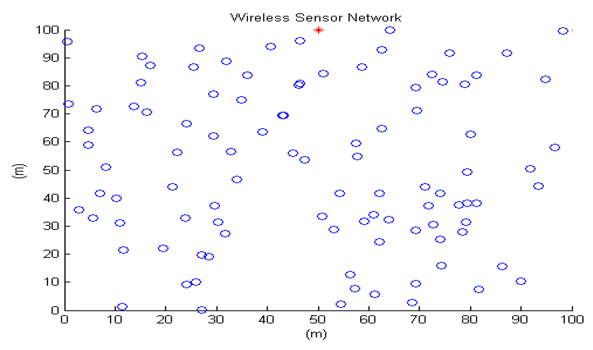
| Area of Network | |
| (Number of Nodes) | 100 |
| (Sink Position) | |
| Packet Size (data) | 4000 bits |
| Hello Packet Size | 200 bits |
| Sink Position | |
| Initial Energy | 0.5 Joules |
| Data Aggregation Energy | 50 pJ/bit/report |
| (Transmitter Electronics) | 50 nJ/bit |
| (Receiver Electronics) | 50 nJ/bit |
| (Transmit Amplifier) | 100 pJ/bit/m2 |
Publisher’s Note: MDPI stays neutral with regard to jurisdictional claims in published maps and institutional affiliations. |
© 2021 by the authors. Licensee MDPI, Basel, Switzerland. This article is an open access article distributed under the terms and conditions of the Creative Commons Attribution (CC BY) license (https://creativecommons.org/licenses/by/4.0/).
Share and Cite
Mukherjee, P.; Pattnaik, P.K.; Al-Absi, A.A.; Kang, D.-K. Recommended System for Cluster Head Selection in a Remote Sensor Cloud Environment Using the Fuzzy-Based Multi-Criteria Decision-Making Technique. Sustainability 2021, 13, 10579. https://doi.org/10.3390/su131910579
Mukherjee P, Pattnaik PK, Al-Absi AA, Kang D-K. Recommended System for Cluster Head Selection in a Remote Sensor Cloud Environment Using the Fuzzy-Based Multi-Criteria Decision-Making Technique. Sustainability. 2021; 13(19):10579. https://doi.org/10.3390/su131910579
Chicago/Turabian StyleMukherjee, Proshikshya, Prasant Kumar Pattnaik, Ahmed Abdulhakim Al-Absi, and Dae-Ki Kang. 2021. "Recommended System for Cluster Head Selection in a Remote Sensor Cloud Environment Using the Fuzzy-Based Multi-Criteria Decision-Making Technique" Sustainability 13, no. 19: 10579. https://doi.org/10.3390/su131910579