
An Efficient Method for Capturing the High Peak Concentrations of PM2.5 Using Gaussian-Filtered Deep Learning

Abstract
1. Introduction
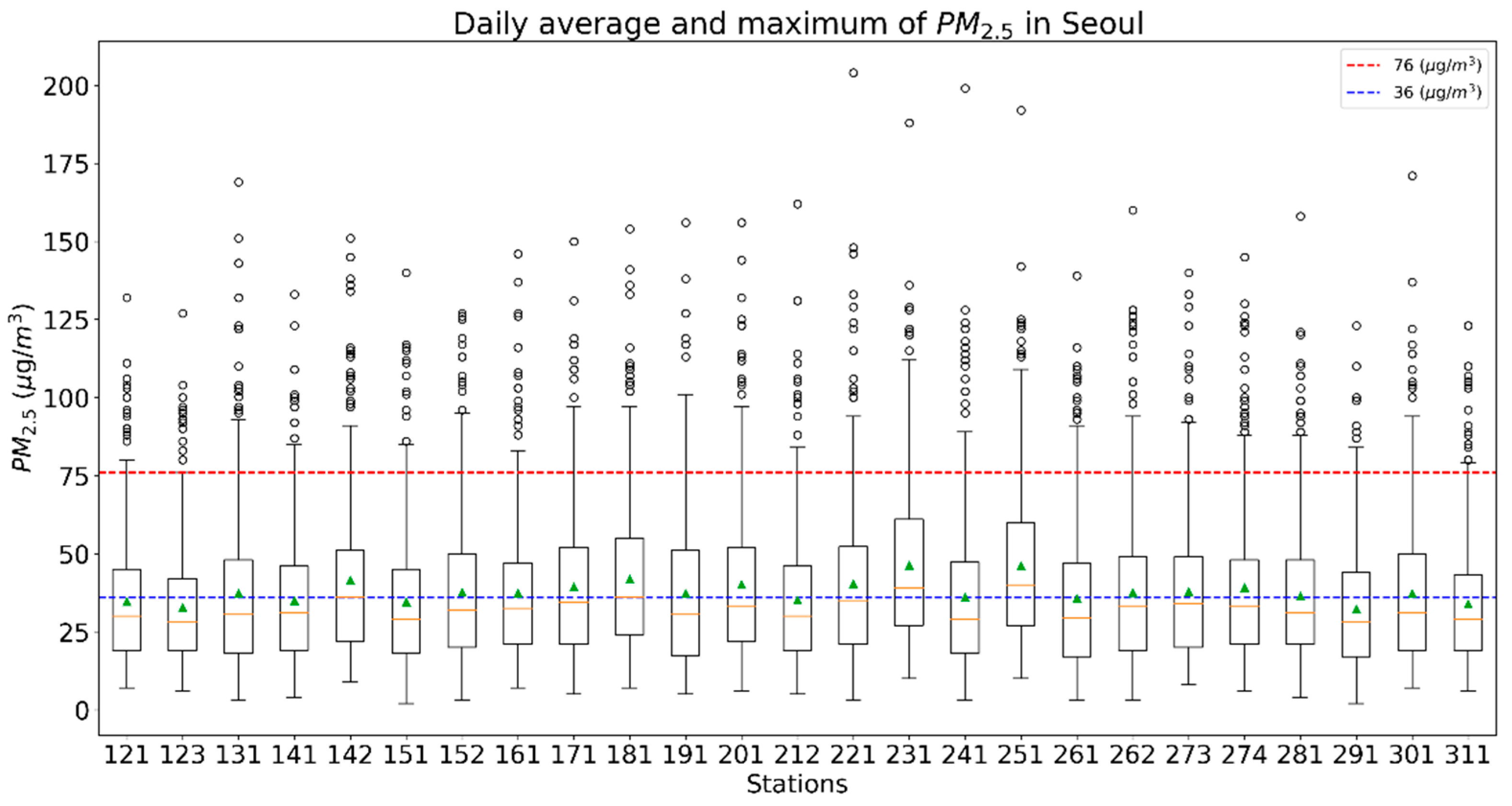
2. Observations
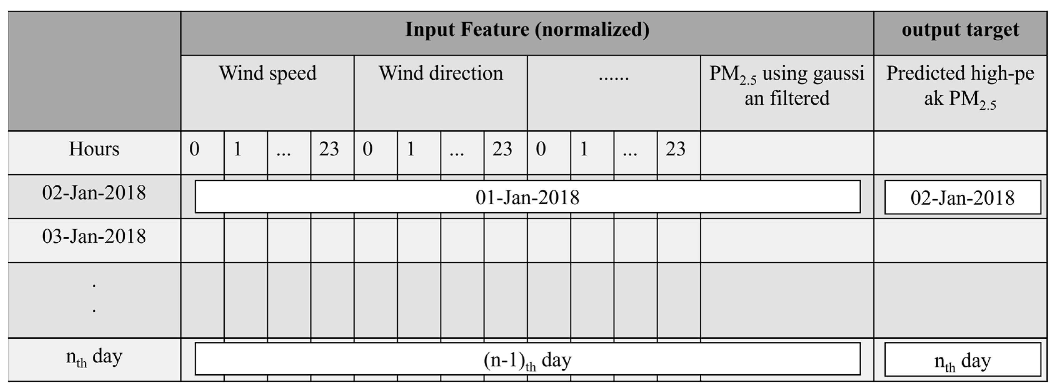
2.1. Preparing Data Used for Predicting Daily Maximum Concentrations of PM2.5
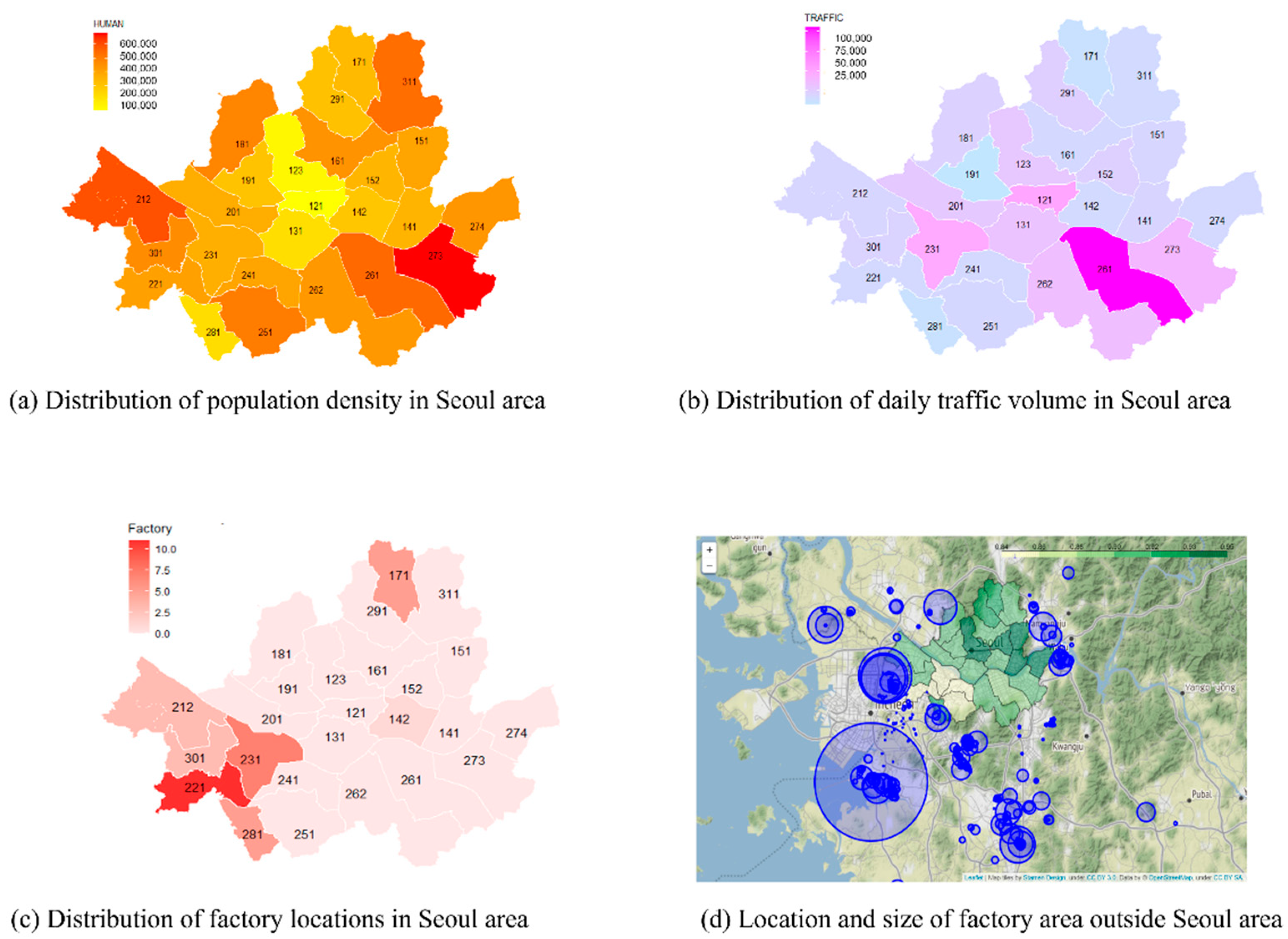
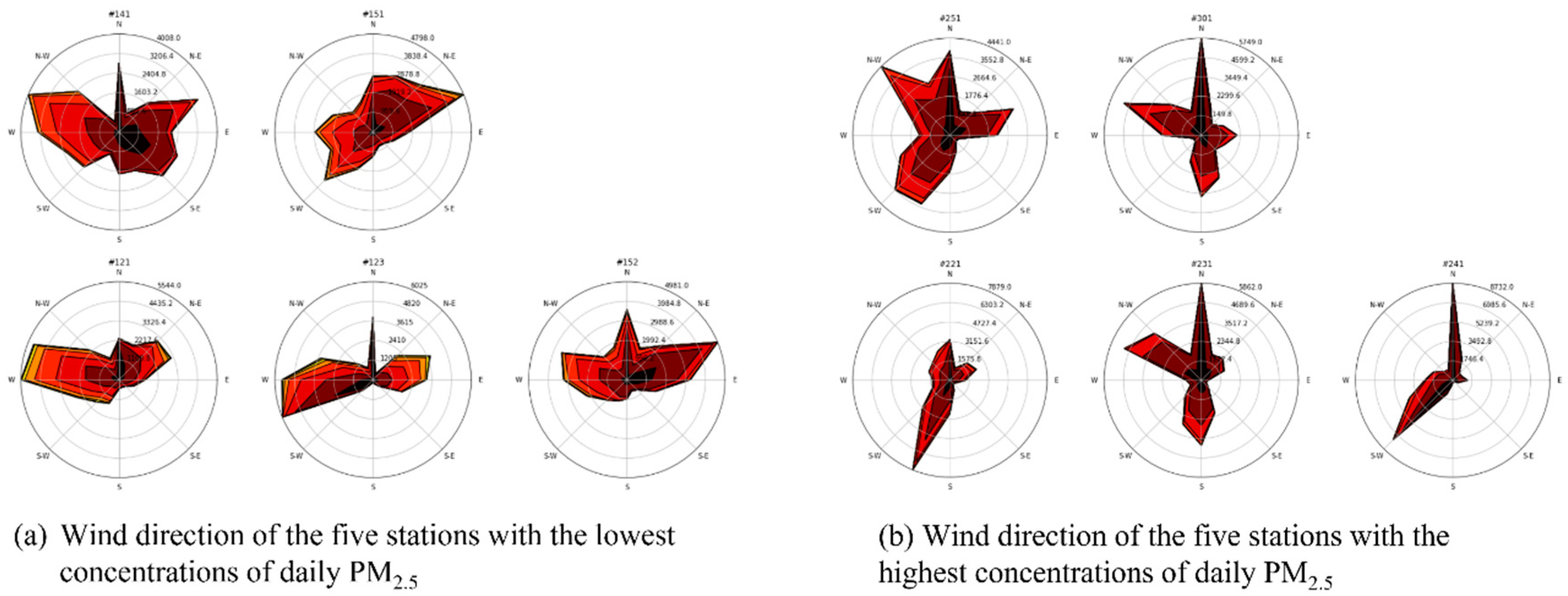
2.2. Correlation between Maximum Daily Concentrations of PM2.5 and Traffic Volume, the Factory Area, and Population Density
3. Materials and Methods
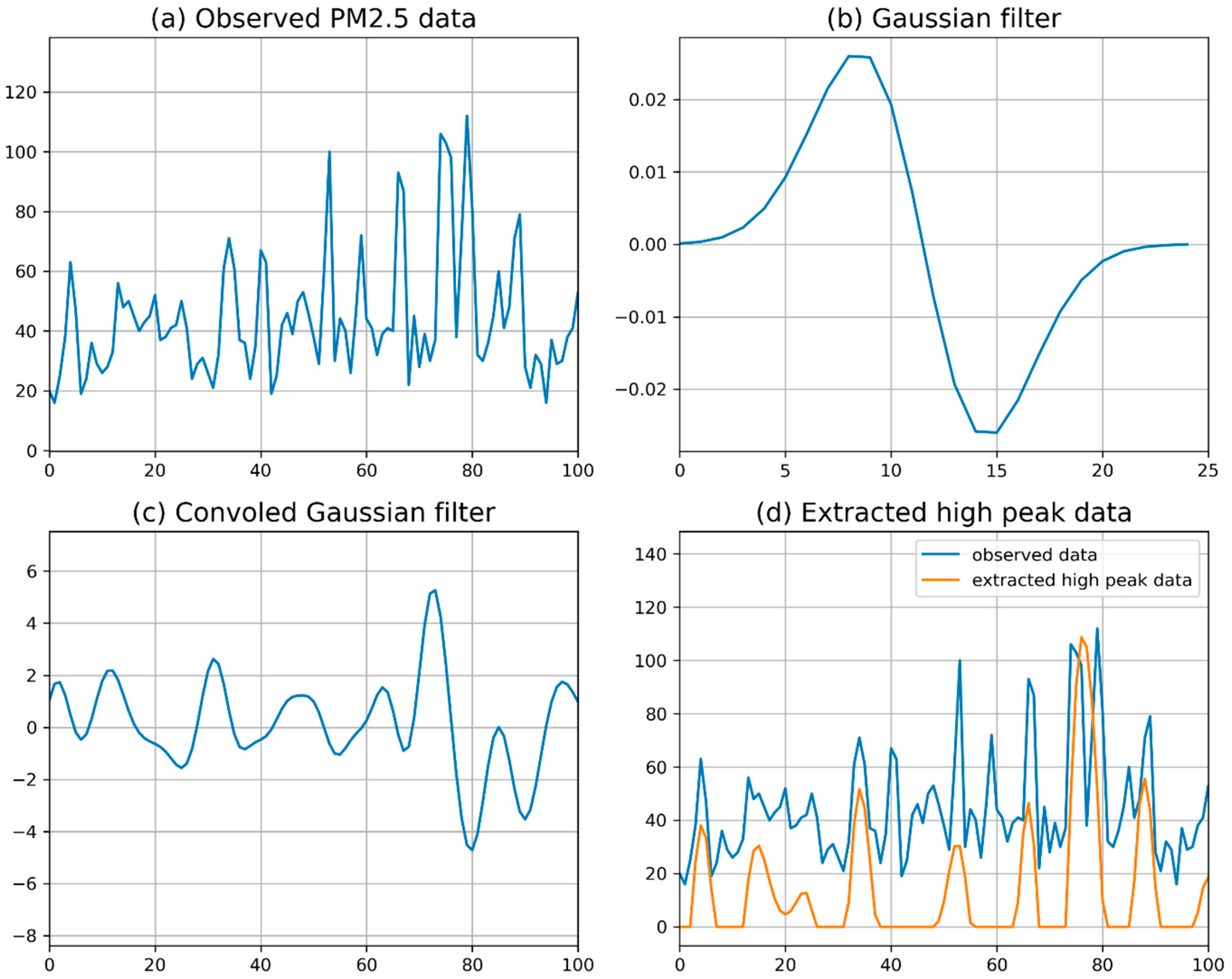
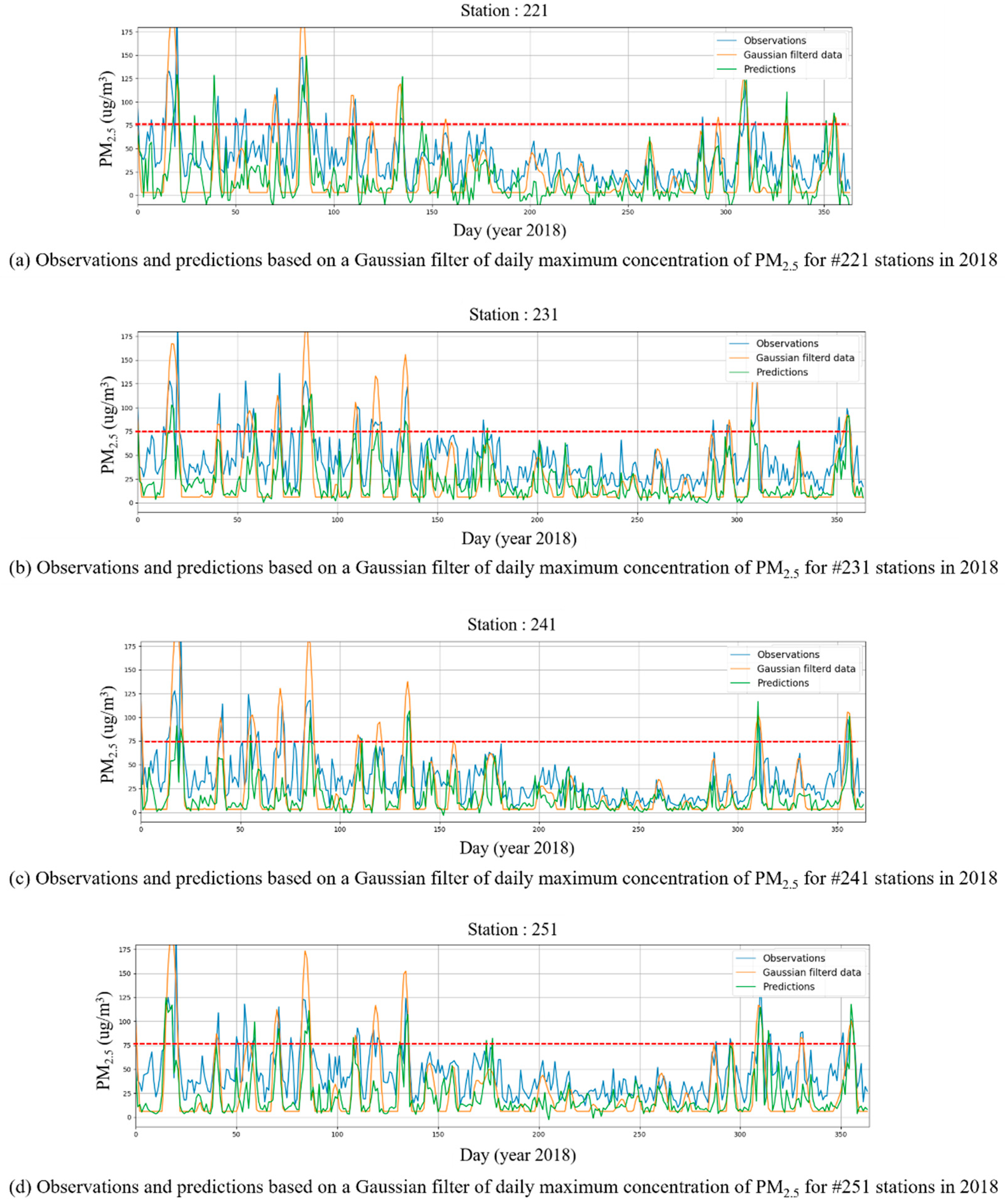
3.1. Outlier Extraction of PM2.5 Data Using a Gaussian Filter
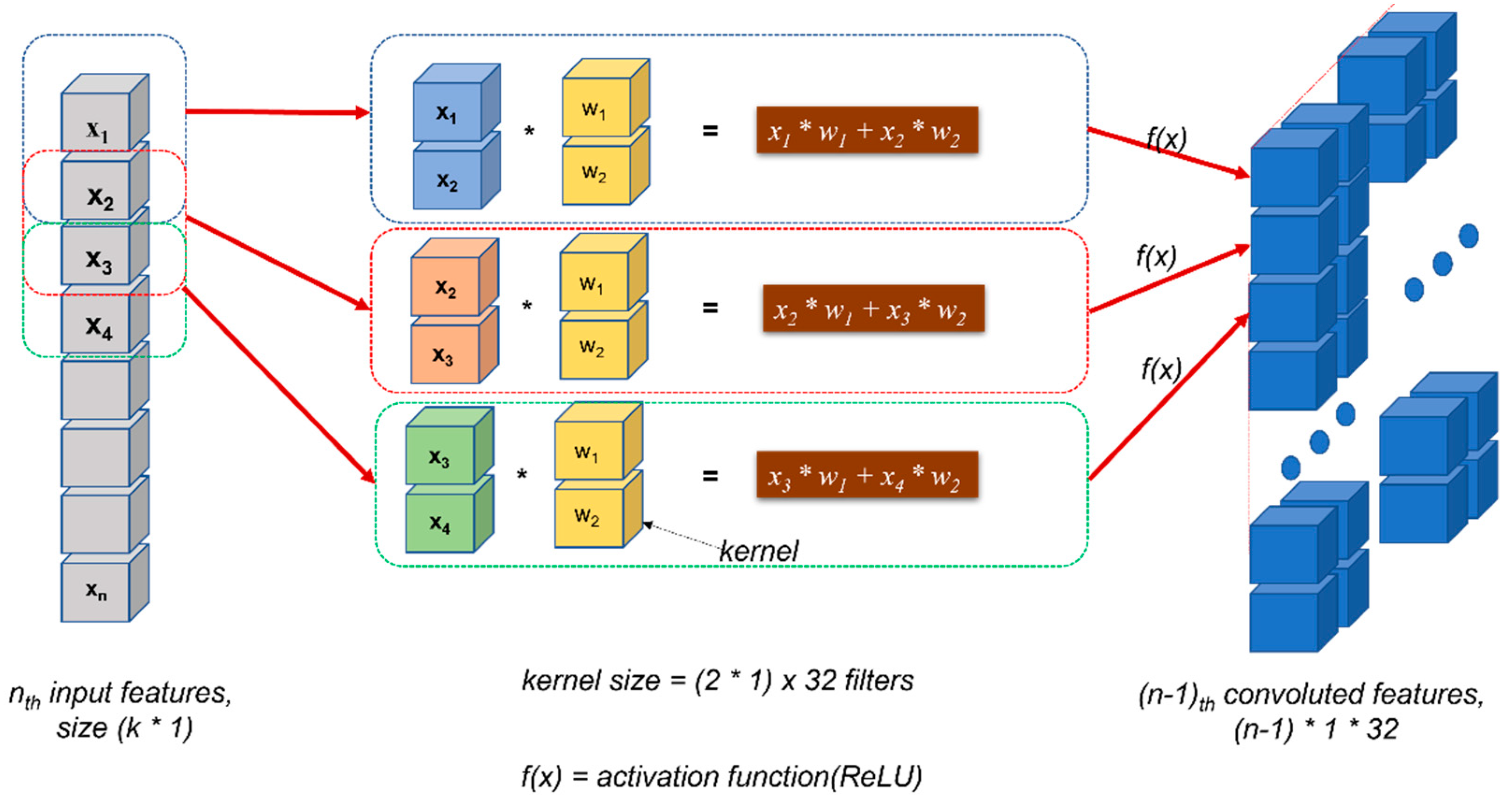
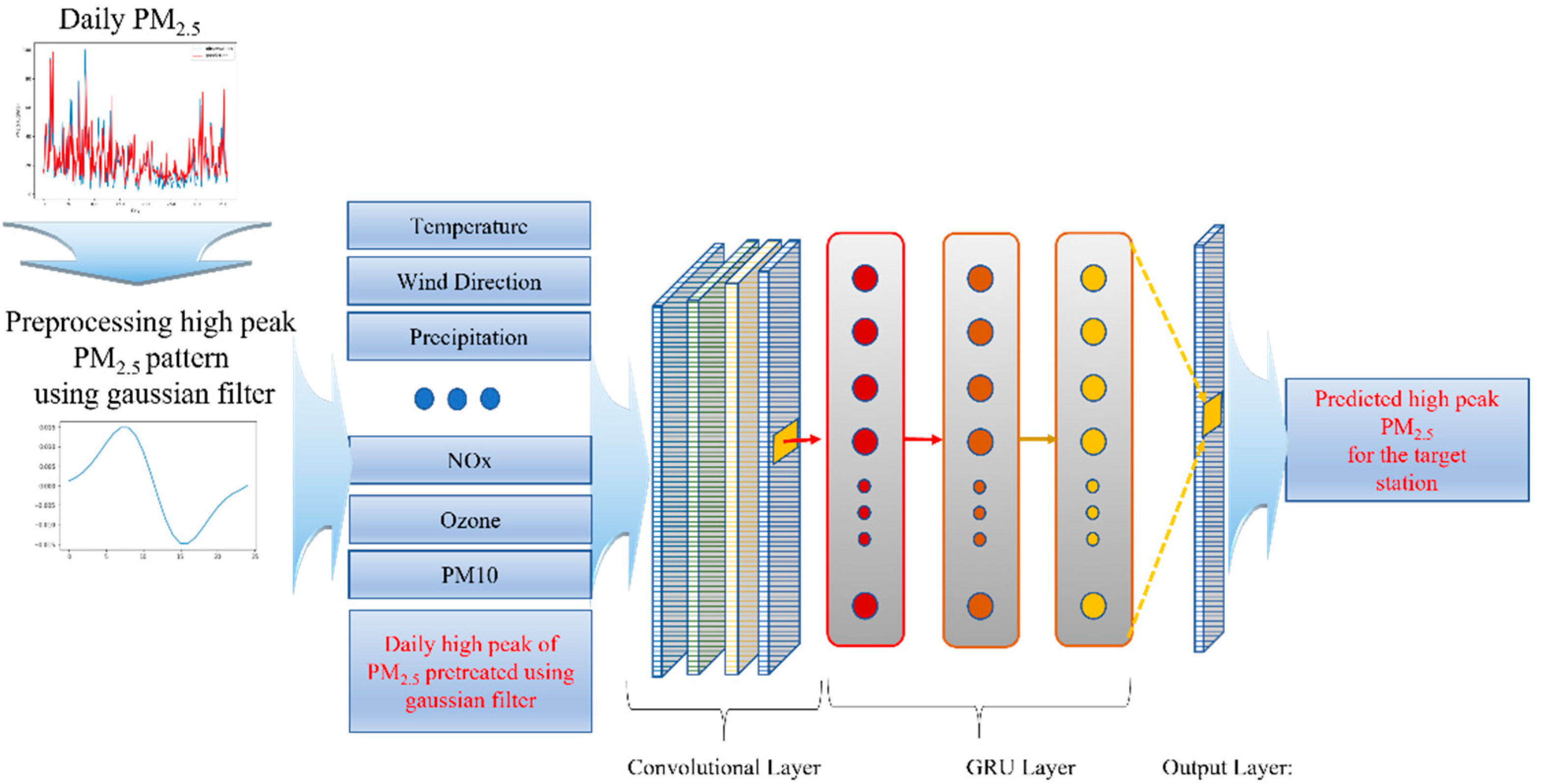
3.2. Deep Learning Architecture
3.3. Model Training and Prediction
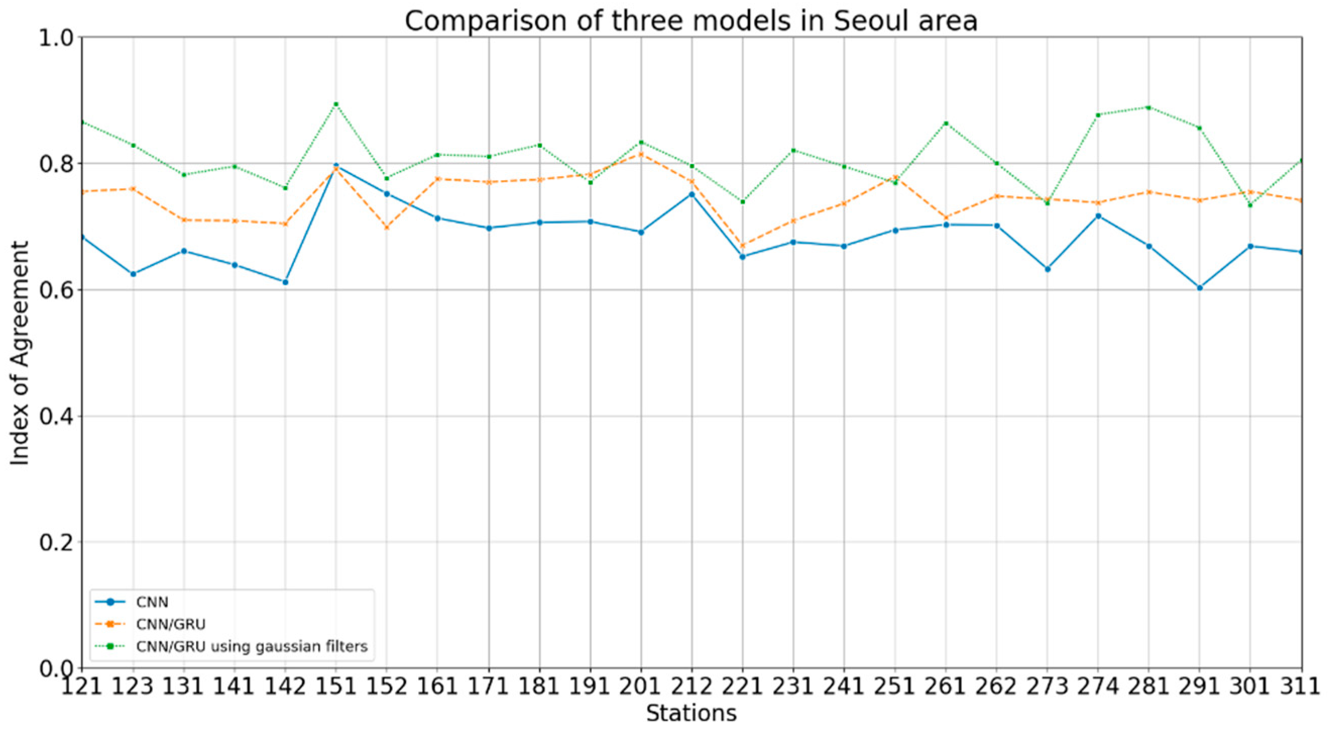
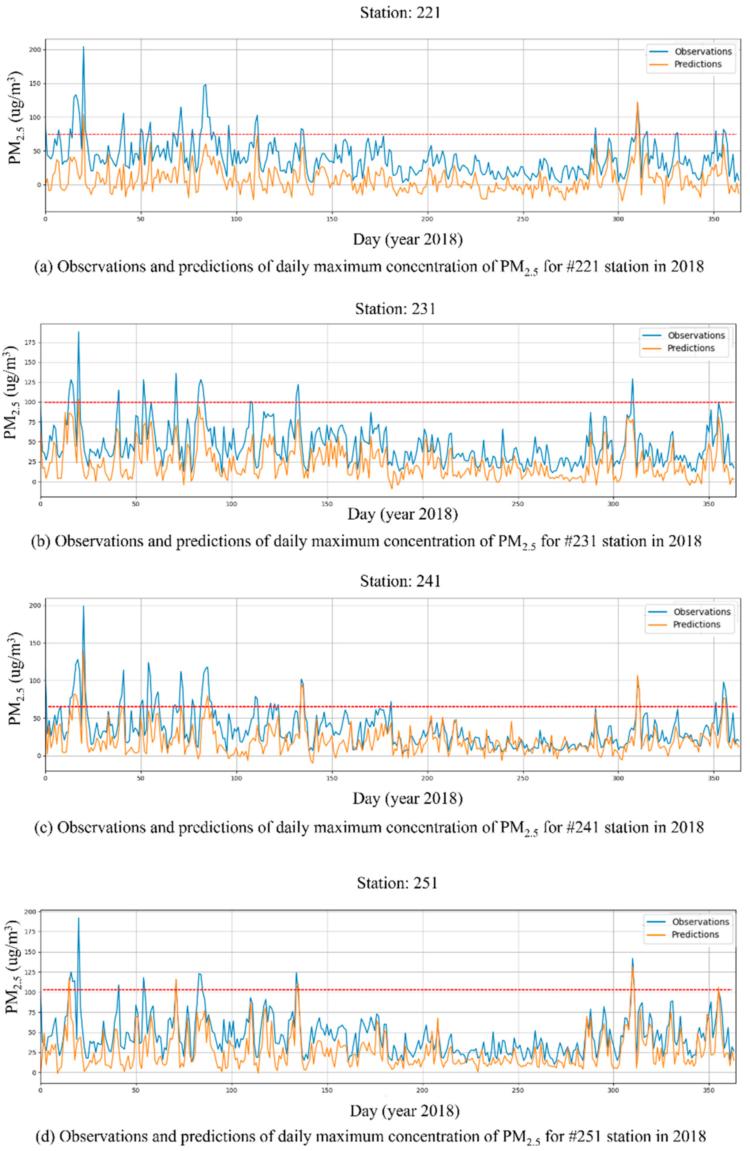
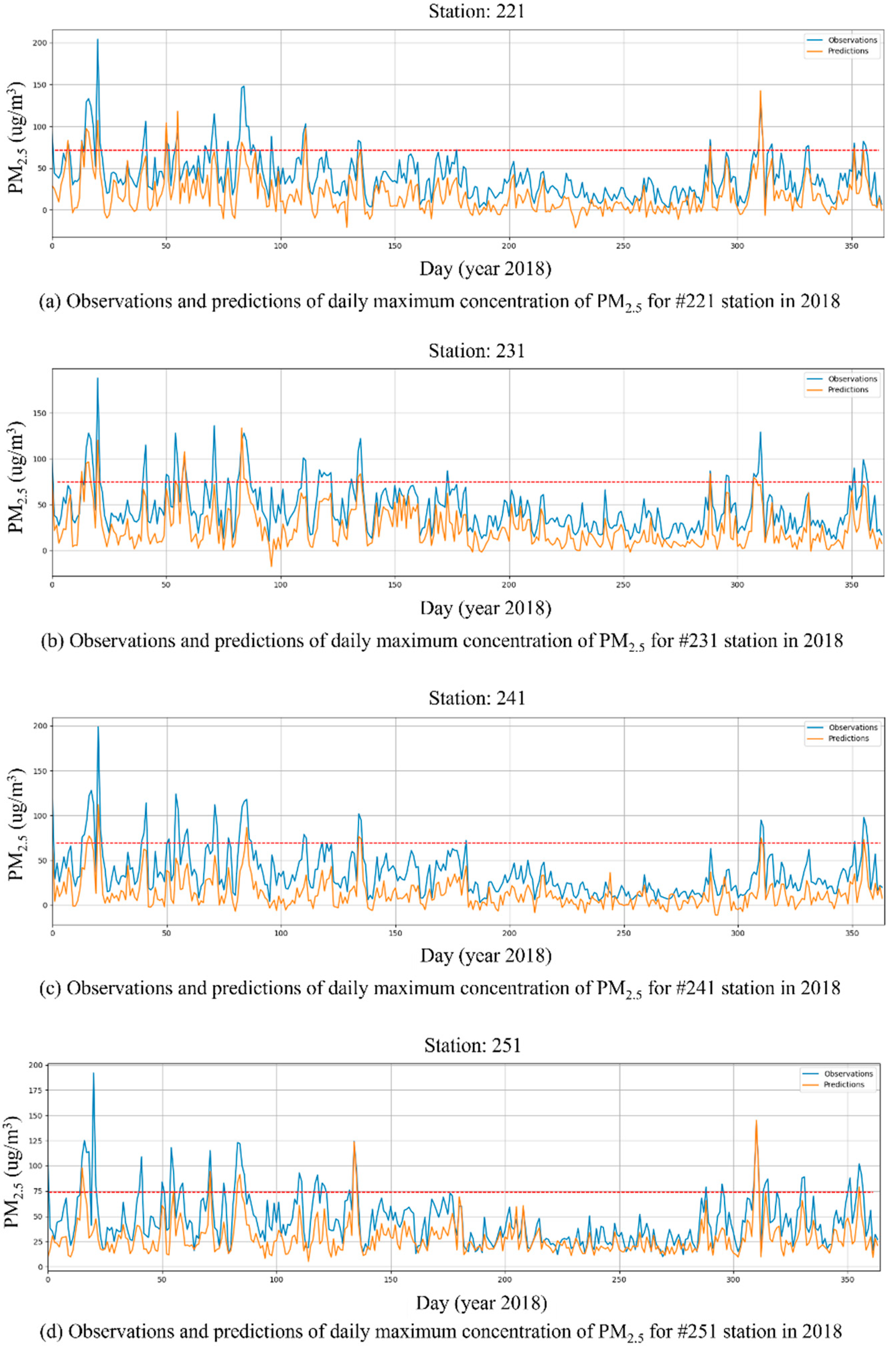
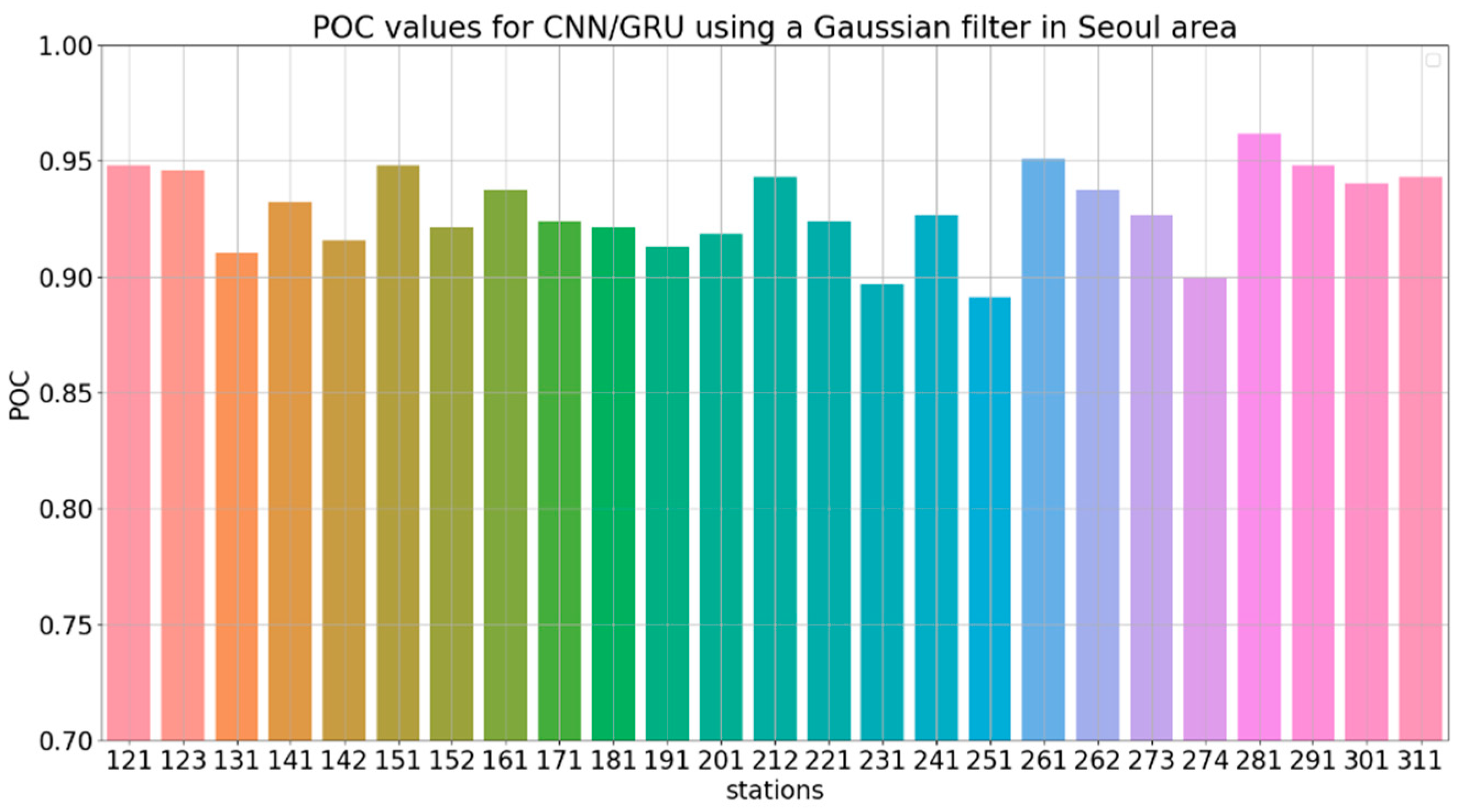
4. Results and Discussion
- Na, number of days when an observation was below the threshold and a prediction was above.
- Nb, number of days when both observations and predictions were above the threshold.
- Nc, number of days when both observations and predictions were below the threshold.
- Na, number of days when an observation was above the threshold and a prediction was below.
5. Conclusions
Author Contributions
Funding
Institutional Review Board Statement
Informed Consent Statement
Data Availability Statement
Acknowledgments
Conflicts of Interest
References
- WHO. Ambient (Outdoor) Air Pollution. 2018. Available online: https://www.who.int/news-room/fact-sheets/detail/ambient-(outdoor)-air-quality-and-health (accessed on 22 September 2021).
- Brunekreef, B.; Holgate, S.T. Air pollution and health. Lancet 2002, 360, 1233–1242. [Google Scholar] [CrossRef]
- Delfino, R.J. Epidemiologic evidence for asthma and exposure to air toxics: Linkages between occupational, indoor, and community air pollution research. Environ. Health Perspect. 2002, 110, 573–589. [Google Scholar] [CrossRef] [PubMed]
- Lanki, T.; Hoek, G.; Timonen, K.L.; Peters, A.; Tiittanen, P.; Vanninen, E.; Pekkanen, J. Hourly variation in fine particle exposure is associated with transiently increased risk of ST segment depression. Occup. Environ. Med. 2008, 65, 782–786. [Google Scholar] [CrossRef]
- Lin, H.; Liu, T.; Xiao, J.; Zeng, W.; Guo, L.; Li, X.; Xu, Y.; Zhang, Y.; Chang, J.J.; Vaughn, M.G.; et al. Hourly peak PM2.5 concentration associated with increased cardiovascular mortality in Guangzhou, China. J. Expo. Sci. Environ. Epidemiol. 2016, 27, 333–338. [Google Scholar] [CrossRef]
- Ebisu, K.; Berman, J.D.; Bell, M.L. Exposure to coarse particulate matter during gestation and birth weight in the U.S. U.S. Environ. Int. 2016, 94, 519–524. [Google Scholar] [CrossRef] [PubMed]
- Yeo, I.; Choi, Y.; Lops, Y.; Sayeed, A. Efficient PM2.5 forecasting using geographical correlation based on integrated deep learning algorithms. Neural Comput. Appl. 2021, 1–17. [Google Scholar] [CrossRef]
- Sayeed, A.; Lops, Y.; Choi, Y.; Jung, J.; Salman, A.K. Bias correcting and extending the PM forecast by CMAQ up to 7 days using deep convolutional neural networks. Atmos. Environ. 2021, 253, 118376. [Google Scholar] [CrossRef]
- Lim, J.H.; Kwak, K.K.; Kim, J.; Jang, Y.K. Analysis of Annual Emission Trends of Air Pollutants by Region. J. Korean Soc. Atmos. Environ. 2018, 34, 76–86, (In Korean with English abstract). [Google Scholar] [CrossRef]
- Kim, J. Assessment and Estimation of Particulate Matter Formation Potential and Respiratory Effects from Air Emission Matters in Industrial Sectors and Cities/Regions. J. Korean Soc. Environ. Eng. 2017, 39, 220–228, (In Korean with English abstract). [Google Scholar] [CrossRef]
- Choe, J.-I.; Lee, Y.S. A Study on the Impact of PM2.5 Emissions on Respiratory Diseases. J. Environ. Policy Adm. 2015, 23, 155, (In Korean with English abstract). [Google Scholar] [CrossRef]
- Kim, Y. Air Pollution in Seoul Caused by Aerosols. J. Korean Soc. Atmos. Environ. 2006, 22, 535–553, (In Korean with English abstract). [Google Scholar]
- Kim, J.; Kang, S. Analysis of Factors Influencing PM10 Pollution in Korea. Proc. J. Korean Soc. Environ. Econ. 2018, 2018, 779–791, (In Korean with English abstract). [Google Scholar]
- Park, S.; Shin, H. Analysis of the Factors Influencing PM2.5 in Korea: Focusing on Seasonal Factors. J. Environ. Policy Adm. 2017, 25, 227–248, (In Korean with English abstract). [Google Scholar] [CrossRef]
- Biancofiore, F.; Busilacchio, M.; Verdecchia, M.; Tomassetti, B.; Aruffo, E.; Bianco, S.; Di Carlo, P. Recursive neu-ral network model for analysis and forecast of PM10 and PM2. 5. Atmos. Pollut. Res. 2017, 8, 652–659. [Google Scholar] [CrossRef]
- Pak, U.; Ma, J.; Ryu, U.; Ryom, K.; Juhyok, U.; Pak, K.; Pak, C. Deep learning-based PM2.5 prediction considering the spatiotem-poral correlations: A case study of Beijing, China. Sci. Total Environ. 2020, 699, 10. [Google Scholar] [CrossRef] [PubMed]
- Kim, H.S.; Park, I.; Song, C.H.; Lee, K.; Yun, J.W.; Kim, H.K.; Jeon, M.; Lee, J.; Han, K.M. Development of a daily PM10 and PM2.5 prediction system using a deep long short-term memory neural network model. Atmos. Chem. Phys. Discuss. 2019, 19, 12935–12951. [Google Scholar] [CrossRef]
- Marloes, E.; Rob, B.; Kees de, H.; Tom, B.; Giulia, C.; Marta, C.; Christophe, D.; Audrius, D.; Evi, D.; Audrey de, N.; et al. Development of Land Use Regression Models for PM2.5, PM2.5 Absorbance, PM10 and PMcoarse in 20 Eu-ropean Study Areas; Results of the ESCAPE Project. Environ. Sci. Technol. 2012, 46, 11205–11215. [Google Scholar]
- LeCun, Y.; Bengio, Y. Convolutional networks for images, speech, and time series. Handb. Brain Theory Neural Netw. 1995, 3361, 1995. [Google Scholar]
- Scarpa, G.; Gargiulo, M.; Mazza, A.; Gaetano, R. A CNN-Based Fusion Method for Feature Extraction from Sentinel Data. Remote Sens. 2018, 10, 236. [Google Scholar] [CrossRef]
- Krizhevsky, A.; Sutskever, I.; Hinton, G.E. ImageNet classification with deep convolutional neural networks. Adv. Neural. Inf. Process. Syst. 2012, 25, 1097–1105. [Google Scholar] [CrossRef]
- Li, X.; Peng, L.; Yao, X.; Cui, S.; Hu, Y.; You, C.; Chi, T. Long short-term memory neural network for air pollutant concentra-tion predictions: Method development and evaluation. Env. Pollut. 2017, 231, 997–1004. [Google Scholar] [CrossRef]
- Cho, K.; van Merrienboer, B.; Gulcehre, C.; Bahdanau, D.; Bougares, F.; Schwenk, H.; Bengio, Y. Learning Phrase Representations using RNN Encoder-Decoder for Statistical Machine Translation, CoRR. arXiv Prepr. 2014, arXiv:1406.1078. [Google Scholar]
- Gers, F.; Schmidhuber, J.; Cummins, F. Learning to Forget: Continual Prediction with LSTM. In Proceedings of the ICANN’99, IEEE, London, UK, 7–10 September 1999; pp. 850–855. [Google Scholar]
- Ravanelli, M.; Brakel, P.; Omologo, M.; Bengio, Y. Light Gated Recurrent Units for Speech Recognition. IEEE Trans. Emerg. Top. Comput. Intell. 2018, 2, 92–102. [Google Scholar] [CrossRef]
- Huang, Y.; Qu, G.; Wei, Z. A new image restoration method by Gaussian smoothing with L1 norm regularization. In Proceedings of the 2012 5th International Congress on Image and Signal Processing, Chongqing, China, 16–18 October 2012; pp. 343–346. [Google Scholar] [CrossRef]
- Batista, G.E.; Monard, M.C. A Study of K-Nearest Neighbor as an Imputation Method. Soft Comput. Syst. Des. Manag. Appl. 2002, 87, 251–260. [Google Scholar]
- Franklin, M.; Koutrakis, P.; Schwartz, J. The Role of Particle Composition on the Association between PM2.5 and Mortality. Epidemiology 2008, 19, 680–689. [Google Scholar] [CrossRef] [PubMed]
- Cho, S.-H.; Kim, P.-R.; Han, Y.-J.; Kim, H.-W.; Yi, S.-M. Characteristics of Ionic and Carbonaceous Compounds in PM2.5 and High Concentration Events in Chuncheon, Korea. J. Korean Soc. Atmos. Environ. 2016, 32, 435–447, (In Korean with English abstract). [Google Scholar] [CrossRef]
- Bae, C.; Yoo, C.; Kim, B.-U.; Kim, H.; Kim, S. PM2.5 Simulations for the Seoul Metropolitan Area: (III) Application of the Modeled and Observed PM2.5 Ratio on the Contribution Estimation. J. Korean Soc. Atmos. Environ. 2017, 33, 445–457, (In Korean with English abstract). [Google Scholar] [CrossRef]
- Yu, G.-H.; Lee, B.-J.; Park, S.-S.; A Jung, S.; Jo, M.R.; Lim, Y.J.; Kim, S. A Case Study of Severe PM2.5 Event in the Gwangju Urban Area during February 2014. J. Korean Soc. Atmos. Environ. 2019, 35, 195–213. [Google Scholar] [CrossRef]
- Lee, H.-J.; Jeong, Y.; Kim, S.-T.; Lee, W.-S. Atmospheric Circulation Patterns Associated with Particulate Matter over South Korea and Their Future Projection. J. Clim. Chang. Res. 2018, 9, 423–433, (In Korean with English abstract). [Google Scholar] [CrossRef]
- Jeon, B.-I. Meteorological Characteristics of the Wintertime High PM10 Concentration Episodes in Busan. J. Environ. Sci. Int. 2012, 21, 815–824, (In Korean with English abstract). [Google Scholar] [CrossRef]
- Wang, M.; Zheng, S.; Li, X.; Qin, X. A new image denoising method based on Gaussian filter. In Proceedings of the 2014 International Conference on Information Science, Electronics and Electrical Engineering, Sapporo, Japan, 26–28 April 2014; Volume 1, pp. 163–167. [Google Scholar]
- Lawrence, S.; Giles, C.L.; Tsoi, A.C.; Back, A.D. Face recognition: A convolutional neural-network approach. IEEE Trans. Neural Netw. 1997, 8, 98–113. [Google Scholar] [CrossRef] [PubMed]
- Gers, F.A.; Schmidhuber, J.; Cummins, F. Learning to Forget: Continual Prediction with LSTM. Neural Comput. 2000, 12, 2451–2471. [Google Scholar] [CrossRef] [PubMed]
- Chollet, F. Keras. 2015. Available online: https://keras.io (accessed on 22 September 2021).
- Pérez, P.; Trier, A.; Reyes, J. Prediction of PM2.5 concentrations several hours in advance using neural networks in Santiago, Chile. Atmos. Environ. 2000, 34, 1189–1196. [Google Scholar] [CrossRef]
- Eder, B.; Kang, D.; Mathur, R.; Yu, S.; Schere, K. An operational evaluation of the Eta–CMAQ air quality forecast model. Atmos. Environ. 2006, 40, 4894–4905. [Google Scholar] [CrossRef]
- Chai, T.; Kim, H.C.; Lee, P.; Tong, D.; Pan, L.; Tang, Y.; Stajner, I. Evaluation of the United States National Air Quality Forecast Capability experimental real-time predictions in 2010 using Air Quality System ozone and NO2 measurements. Geosci. Model Dev. 2013, 6, 1831–1850. [Google Scholar] [CrossRef]


| Wind Speed (miles/hour) | Wind Direction (Degrees Compass) | Temperature | Relative Humidity (percent) | …… | NOx (ppb) | Preprocessed PM2.5 Using Gaussian Filter | |
|---|---|---|---|---|---|---|---|
| 1 January 2015 0:00 | |||||||
| 1 January 2015 1:00 | |||||||
| : : | |||||||
| 31 December 2017 23:00 |
| Station # | CNN | CNN/GRU | CNN/GRU w/Gaussian Filters | ||||||
|---|---|---|---|---|---|---|---|---|---|
| IOA | r | MAE | IOA | r | MAE | IOA | r | MAE | |
| 121 | 0.68 | 0.55 | 0.11 | 0.75 | 0.64 | 0.09 | 0.87 | 0.75 | 0.08 |
| 123 | 0.62 | 0.44 | 0.11 | 0.76 | 0.67 | 0.09 | 0.83 | 0.71 | 0.08 |
| 131 | 0.66 | 0.55 | 0.08 | 0.71 | 0.59 | 0.08 | 0.78 | 0.74 | 0.06 |
| 141 | 0.64 | 0.45 | 0.12 | 0.71 | 0.52 | 0.12 | 0.79 | 0.68 | 0.09 |
| 142 | 0.61 | 0.46 | 0.09 | 0.70 | 0.62 | 0.08 | 0.76 | 0.65 | 0.08 |
| 151 | 0.80 | 0.68 | 0.09 | 0.79 | 0.67 | 0.09 | 0.89 | 0.83 | 0.07 |
| 152 | 0.75 | 0.63 | 0.09 | 0.70 | 0.63 | 0.08 | 0.78 | 0.68 | 0.08 |
| 161 | 0.71 | 0.58 | 0.09 | 0.78 | 0.67 | 0.08 | 0.81 | 0.75 | 0.07 |
| 171 | 0.70 | 0.52 | 0.11 | 0.77 | 0.65 | 0.09 | 0.81 | 0.70 | 0.09 |
| 181 | 0.71 | 0.58 | 0.09 | 0.77 | 0.72 | 0.08 | 0.83 | 0.76 | 0.07 |
| 191 | 0.71 | 0.62 | 0.09 | 0.78 | 0.70 | 0.08 | 0.77 | 0.73 | 0.07 |
| 201 | 0.69 | 0.54 | 0.09 | 0.81 | 0.69 | 0.08 | 0.83 | 0.71 | 0.08 |
| 212 | 0.75 | 0.59 | 0.11 | 0.77 | 0.65 | 0.09 | 0.80 | 0.64 | 0.09 |
| 221 | 0.65 | 0.48 | 0.11 | 0.67 | 0.56 | 0.10 | 0.74 | 0.62 | 0.09 |
| 231 | 0.67 | 0.49 | 0.12 | 0.71 | 0.63 | 0.10 | 0.82 | 0.74 | 0.09 |
| 241 | 0.67 | 0.55 | 0.10 | 0.74 | 0.66 | 0.09 | 0.79 | 0.71 | 0.08 |
| 251 | 0.69 | 0.51 | 0.11 | 0.78 | 0.68 | 0.09 | 0.77 | 0.71 | 0.08 |
| 261 | 0.70 | 0.55 | 0.10 | 0.71 | 0.64 | 0.09 | 0.86 | 0.79 | 0.08 |
| 262 | 0.70 | 0.61 | 0.09 | 0.75 | 0.59 | 0.09 | 0.80 | 0.66 | 0.09 |
| 273 | 0.63 | 0.57 | 0.10 | 0.74 | 0.69 | 0.08 | 0.74 | 0.65 | 0.08 |
| 274 | 0.72 | 0.57 | 0.10 | 0.74 | 0.65 | 0.09 | 0.88 | 0.78 | 0.07 |
| 281 | 0.67 | 0.52 | 0.11 | 0.75 | 0.62 | 0.10 | 0.89 | 0.81 | 0.07 |
| 291 | 0.60 | 0.44 | 0.10 | 0.74 | 0.58 | 0.09 | 0.86 | 0.75 | 0.07 |
| 301 | 0.67 | 0.53 | 0.11 | 0.76 | 0.63 | 0.09 | 0.73 | 0.66 | 0.09 |
| 311 | 0.66 | 0.49 | 0.10 | 0.74 | 0.58 | 0.10 | 0.80 | 0.70 | 0.07 |
Publisher’s Note: MDPI stays neutral with regard to jurisdictional claims in published maps and institutional affiliations. |
© 2021 by the authors. Licensee MDPI, Basel, Switzerland. This article is an open access article distributed under the terms and conditions of the Creative Commons Attribution (CC BY) license (https://creativecommons.org/licenses/by/4.0/).
Share and Cite
Yeo, I.; Choi, Y. An Efficient Method for Capturing the High Peak Concentrations of PM2.5 Using Gaussian-Filtered Deep Learning. Sustainability 2021, 13, 11889. https://doi.org/10.3390/su132111889
Yeo I, Choi Y. An Efficient Method for Capturing the High Peak Concentrations of PM2.5 Using Gaussian-Filtered Deep Learning. Sustainability. 2021; 13(21):11889. https://doi.org/10.3390/su132111889
Chicago/Turabian StyleYeo, Inchoon, and Yunsoo Choi. 2021. "An Efficient Method for Capturing the High Peak Concentrations of PM2.5 Using Gaussian-Filtered Deep Learning" Sustainability 13, no. 21: 11889. https://doi.org/10.3390/su132111889
APA StyleYeo, I., & Choi, Y. (2021). An Efficient Method for Capturing the High Peak Concentrations of PM2.5 Using Gaussian-Filtered Deep Learning. Sustainability, 13(21), 11889. https://doi.org/10.3390/su132111889