
Multidimensional Aspects of Sustainable Biofuel Feedstock Production


1
Department of Biosystems and Agricultural Engineering, Michigan State University, East Lansing, MI 48824, USA
2
Department of Electrical and Computer Engineering, Michigan State University, East Lansing, MI 48824, USA
*
Author to whom correspondence should be addressed.
Sustainability 2021, 13(3), 1424; https://doi.org/10.3390/su13031424
Submission received: 26 December 2020
/
Revised: 25 January 2021
/
Accepted: 26 January 2021
/
Published: 29 January 2021
(This article belongs to the Special Issue Sustainable Water Quality Management in the Changing Environment)
Abstract
:Bioenergy is becoming increasingly relevant as an alternative to fossil fuels. Various bioenergy feedstocks are suggested as environmentally friendly solutions due to their positive impact on stream health and ability to sequester carbon, but most evaluations for bioenergy feedstocks have not evaluated the implications of bioenergy crop production holistically to date. Through the application of multi-objective optimization on 10 bioenergy feedstock rotations in a Michigan watershed, a Pareto front is searched to identify optimal trade-off solutions for three objective functions representing stream health, environmental emissions/carbon footprint, and economic feasibility. Various multi-criteria decision-making techniques are then applied to the resulting Pareto front to select a set of most-preferred trade-off solutions, which are compared to optimal solutions from each individual objective function. The most-preferred trade-off solutions indicate that a diverse mix of rotations are necessary to optimize all three objectives, whereas the individually optimal solutions do not consider a diverse range of feedstocks, thereby making the proposed multi-objective treatment an important and pragmatic strategy.

1. Introduction
The U.S. Energy Information Administration (EIA) predicts that global energy consumption will increase 50% by 2050 [1]. In efforts to reach this demand in a sustainable way around the world, affordable clean energy was included in the Sustainable Development Goals adopted by all United Nations Member States in 2015 [2]. Innovation and production of renewable energy have been growing around the world, with 29% of the global electricity capacity [3] and 3% of transportation fuels [4] accounted for by renewables in 2018. Currently, hydropower, wind, and solar make up the majority of the renewable electricity sector, while biofuels account for all of the renewable transportation fuels [3].
In 2005, the U.S. Department of Energy set a series of goals, including the production of 36 billion gallons of renewable fuel by 2022 [5]. They projected that over 30% of the 2005 U.S. petroleum consumption could be displaced by one billion tons of dry biomass, sustainably produced on an annual basis in the U.S., without threatening the food and feed supply [6]. Biofuel production would be beneficial in the U.S. to decrease dependency on foreign oil, help to mitigate climate change, create jobs, and diversify domestic energy sources [7,8]. Meanwhile, negative environmental impacts from land use change, greenhouse gas (GHG) emissions, and decreased biodiversity from increased corn-based ethanol production have already been observed [9,10].
When developing a sustainable and cost-effective alternative to current agricultural practices, multiple aspects of large-scale bioenergy crop production must be considered [7,11]. These aspects include stream health, life cycle analysis (i.e., environmental emissions), and economic feasibility considerations. For instance, nutrient leaching, erosion, and decreased water holding capacity are all increasingly apparent problems faced by farmers due to deteriorating soil quality around the U.S., especially in heavily cultivated states in the Midwest [12]. It has been observed that soil organic matter, required for nutrient retention, erosion control, and water holding capacity, is heavily impacted by conventional agricultural practices [13]. In addition, eutrophication occurs as a result of excess nutrients in the water originated from agricultural runoff, being a potent ecological stressor, which has been shown to greatly impact fish fitness and populations, deteriorating stream health [14]. Incorporating rotations can decrease nutrient leaching through varied nutrient utilization [15]. Likewise, the incorporation of perennial and cover crops with living root systems in the fall season can decrease nutrient leaching by utilizing nutrients and water during the wet periods [16]. On the other hand, approximately 76% of all GHG emissions in the U.S. were attributed to burning fossil fuels in 2017 [17]. Even though the combustion of fuel will always lead to GHG emissions, bioenergy crop cultivation counteracts the emissions by taking in carbon dioxide through photosynthesis to produce biomass. Production and combustion of biofuels generates a closed-loop system between carbon sequestering feedstock production, conversion into fuel, and combustion emissions. For instance, Argonne National Laboratory estimates that biofuels can reduce atmospheric GHG produced by emissions up to 115% when compared to gasoline [18]. It is worth noting that the life cycle analysis (LCA) of bioenergy crops is largely influenced by the above- to below-ground biomass ratio. Perennial grasses, such as switchgrass and miscanthus, have large quantities of below-ground biomass, allowing for greater carbon sequestration through both biomass and soil organic carbon production [19]. Regarding economic factors, there is already a strong market for bioenergy products in the U.S. Particularly, Michigan is in the top 20% of states for ethanol consumption and biomass feedstock electricity [20]. That being said, corn kernels are currently the primary biofuel feedstock [21]. Conversion of cellulosic feedstocks, such as corn stover, switchgrass, and miscanthus, requires additional pretreatment processes, which have not yet been widely implemented on a large scale [22]. Even though perennial bioenergy feedstocks tend to be less energy-intensive than conventional crops once established [23], their lower market value must be taken into account when optimizing for sustainable bioenergy feedstock production [24].
Stream health, life cycle analysis, and economic feasibility must be taken into account to provide policymakers and stakeholders with an environmentally feasible solution for agricultural land use. Therefore, in this study, agricultural land use for bioenergy feedstocks is optimized considering macroinvertebrate- and fish-based stream health indicators, environmental emissions (total nitrogen, total phosphorus, sediments, and sequestrated carbon), and net economic return. Studies have been conducted on the potential for bioenergy feedstock cultivation [25,26,27], but they do not consider all the aforementioned aspects simultaneously. This work aims to take all three key dimensions (i.e., stream health, life cycle analysis, and economic feasibility) into account to optimize for the most sustainable bioenergy cultivation solution in the Honeyoey Creek-Pine Creek watershed in Michigan, U.S. The objectives of this study are to design a novel framework which incorporates the linkages and feedbacks among land use change due to biofuels feedstock production, stream health, environmental benefits, economic return, and optimization techniques. Multi-objective optimization within the framework aims to maximize the benefits of biofuel feedstock production, while minimize potential negative environmental consequences to generate quantitative support for consensus decision-making models. The three objectives of this study were to (1) characterize the mechanism(s) by which atmospheric, terrestrial, and in-stream variables affect aquatic ecological integrities (fish and macroinvertebrate communities) and water quality; (2) establish a framework that quantifies the overall environmental impacts of land use change; and (3) develop a multi-objective optimization tool for the selection and placement of bioenergy crops.
2. Materials and Methods
2.1. Study Area
The Honeyoey Creek-Pine Creek watershed (Hydrologic Unit Code 0408020202) is located in the Saginaw River watershed in Michigan, U.S. (Figure 1). The Saginaw River watershed is identified as an Area of Concern by the U.S. Environmental Protection Agency (EPA) [28]. Nonpoint pollution control is one of the main priorities for action, due to the high level of contaminated sediments detected and degraded fisheries observed in the watershed. Currently, agriculture is the dominant land use within the study area, taking up approximately 52% of the 1100 km2 land area followed by forests (~23%), wetlands (~17%), pasturelands (~5%), and urban (~3%). The domination of agricultural land within the region has a profound impact on stream health, economy, and the surrounding environment.
2.2. Modeling Process Overview
This study focuses on bioenergy feedstock production in Michigan, the third most agriculturally diverse state in the U.S., which also has high interest in bioenergy feedstocks [29]. An overview of the models and optimization process can be seen in Figure 2. Four models (i.e., hydrological model, stream health model, life cycle assessment, and economic model) were used to generate three scores (i.e., stream heath, environmental, and economic scores) for multi-objective optimization of bioenergy feedstock production in the study area. Figure 2 shows the inputs and outputs associated with each model. First, a hydrological model was calibrated and validated using climatological and physiographical data for the Honeyoey Creek-Pine Creek watershed. Ten bioenergy crop rotations were then simulated by the hydrological model. The output of the hydrological model includes daily values for streamflow and sediment and nutrient (total nitrogen and phosphorus) loads that resulted from bioenergy crop selection and placement within the study area in a 12-year period. Then, key ecologically-relevant hydrologic indicators were obtained from the simulated daily streamflow time-series in order to feed the stream health model, which represents the impact on freshwater ecological integrity in terms of macroinvertebrates and fish-based indicators.
A life cycle assessment was also conducted on all ten bioenergy crop rotations and paired with the corresponding sediment, total nitrogen, and total phosphorus loads from the hydrological model to develop an environmental score. An economic model was used to calculate the average annual net return associated with each bioenergy crop over a 12-year period. The three resulting scores were then fed into a multi-objective optimization algorithm, which generated a set of Pareto-optimal solutions. The developed GIS-based multi-criteria decision system and optimization can be used by policymakers and stakeholders to guide bioenergy crop selection and placement to maximize economic return while minimizing potential negative stream health and environmental impacts.
2.3. Stream Health Indicator
2.3.1. Hydrological Model Description
The impact of bioenergy crops on water resources was analyzed using the Soil and Water Assessment Tool (SWAT, rev. 622), which is a hydrological model developed by Arnold et al. [30] for the United States Department of Agriculture, Agricultural Research Service (USDA, ARS). SWAT uses both physiographical and climatological data to simulate water movement and pollutant transport through watersheds. In the Honeyoey Creek-Pine Creek watershed, the most important observations are changes in streamflow and movement of nutrients, pesticides, and sediments [30,31], which all vary with land use [32]. The inputs of SWAT are used to estimate erosion and sediment transport via runoff through the Modified Universal Soil Loss Equation (MUSLE) [33]. Additionally, the nitrogen cycle and phosphorus cycle are integrated to estimate the movement of nutrients via both runoff and lateral subsurface flow [33].
In order for SWAT to produce a reliable watershed model, data on both the physiographical and climatological characteristics of the watershed were required. First, data as related to the physical characteristics of the watershed, such as topography, soil type, and land use were acquired from different resources. Concerning the topography, the U.S. Geological Survey (USGS) National Elevation Dataset (NED) at 30-m resolution provided topographical information for the watershed [34]. Soil data were obtained through the USDA Natural Resource Conservation Service (NRCS) SSURGO database, which varies in scale of accuracy between 1:12,000 and 1:63,360 [35]. Land use data were provided by the USDA Cropland Data Layer for the study period at 30-m resolution [36]. Climatological data from the period of the study, 2003–2014, were also collected for model development from the National Climate Data Center (NCDC). Daily precipitation and maximum and minimum temperatures were used from 16 weather stations within the watershed [37].
2.3.2. Hydrological Model Calibration and Validation
Both calibration and validation were performed on the SWAT model using observed flow to ensure model accuracy. Calibration is the act of adjusting model parameters to produce outputs that are comparable to observed data within the same time-frame, whereas validation evaluates how the calibrated model parameters fit observed data outside of the time-frame used for calibration [30]. Data from 2003–2008 was used for calibration, while data from 2009–2014 was used for validation. Accuracy was evaluated using eight different statistical measures: Nash–Sutcliffe efficiency (NSE), Kling–Gupta efficiency (KGE), modified KGE-statistic (KGE’), ratio of the root mean square error to the standard deviation of measured data (RSR), index of agreement (d), coefficient of determination (R2), percent bias (PBIAS), and root mean square error (RMSE cms) [38,39,40]. Observed values used for daily streamflow calibration/validation were collected from the Pine River Near Midland USGS gauging station (ID 04155500). At the same time, the results of the model calibration/validation are presented in Table S1 in Supplementary Materials. Due to the lack of water quality stations within the area of study, water quality model parameters were taken from a previously calibrated SWAT model for the Saginaw River watershed [41].
2.3.3. Bioenergy Crops Implementation
Ten bioenergy crop rotations were considered for agricultural land in the Honeyoey Creek-Pine Creek watershed. Corn, corn-stover, corn-soy rotation, corn-stover-soy rotation, soybean, corn-soy-canola, sorghum, sorghum-soy, miscanthus, and switchgrass were all considered. The SWAT model divided the watershed into subbasins, which were further divided into Hydrologic Response Units (HRUs). HRUs are geographic units with distinctive land use, soil, and slope features [42]. In this study, it was assumed that there was one HRU per subbasin and the ten bioenergy crops were the only crops grown in the Honeyoey Creek-Pine Creek watershed. This simplification allowed for the complex multi-objective optimization even though the crop distribution is not commonly observed in Michigan. Corn, corn-stover, corn-soy rotation, corn-stover-soy rotation, soybean, corn-soy-canola, sorghum, sorghum-soy, miscanthus, and switchgrass were all considered. For each rotation, tilling practices were assumed to be conservative with disk cultivators followed by soil finishers. Corn, soy, and canola were assumed to be glyphosate resistant. Fertilizer rates were based on recommendations from Michigan State University Extension field studies [29,43,44,45] rather than current soil makeup for each agricultural field. Additionally, synthetic fertilizers were the only assumed nutrient input. All fields were assumed to consist of 1.75% soil organic matter, as suggested for central Michigan [46].
Both corn and corn-stover consisted of five years of corn and one-year soybean, with the corn leaving the stover on the field during the winter dormant period and corn-stover harvesting 38% of post-corn grain harvest biomass and requiring additional fertilizer [47,48]. Continuous soybean consisted of two years of soy, followed by one year of corn. The corn-soy and corn-stover-soy rotation were similar with corn in the first year followed by soy in the second. Again, 38% of stover was harvested after corn grain harvest in the corn-stover-soy rotations, which was supplemented with additional fertilizers. Phosphorus was applied bi-annually during the soybean year of the rotation and was considered to remain on the field for the corn, reducing potential leaching into waterbodies [49]. During the corn-soy-canola rotation, the corn and soy were planted similarly to the corn-soy rotation, with the third year being a winter canola variety planted in the fall, after soybean harvest, and harvested in the late spring [50]. Sorghum had an operation schedule similar to corn with five years of sorghum followed by one year of soy. Fertilizer, herbicide, and seeding rate for this crop were all based on suggestions from the University of Wisconsin Extension office [51]. Sorghum was planted in the late spring when the ground was between 15.5–18.5 °C about three weeks after corn [51]. The sorghum-soy rotation alternated sorghum and soy on a yearly basis with similar additives to the sorghum rotation and soy rotation. Both miscanthus and switchgrass were scheduled based on a 12-year lifespan with the first three years dedicated to the establishment [29]. Both perennials were planted in the first year then had supplementary seeding in the second year before becoming fully robust in the third. Herbicides, fertilizer, and seeding rate were all based on suggestions from MSU Extension [29].
2.3.4. Stream Health Model
Fuzzy logic methods are robust for modeling stream health, due to their ability to model complex and non-linear systems [52,53,54]. The fuzzy logic methods use graphical membership functions (MFs) to describe the importance of a degree of membership from 0 (no membership) to 1 (full membership). An adaptive neuro-fuzzy inference system (ANFIS) is a fusion method, which uses artificial neural networks (ANN) to build optimal fuzzy logic (MFs) [55]. This method was used for this study due to being advantageous for evaluating ecological systems [56,57]. Previously developed ANFIS models produced by Woznicki et al., 2016 were adapted for the Honeyoey Creek-Pine Creek study area. Both linear and non-linear shapes were tested for best fit, including trapezoidal, triangular, Gaussian, Gaussian composite, and generalized bell. The most fitting shape was generated as a final set of linear and constant MFs, which were extracted as the stream health score for each scenario. Since flow is a “master variable” in ecohydrological studies as flow regime alteration can significantly impact stream health and aquatic life [58], ecologically-relevant hydrologic indicators were identified as key explanatory variables for predicting different macroinvertebrate- and fish-based indicators.
The macroinvertebrate indicators included the number of Ephemeroptera, Plecoptera, and Trichoptera (EPT) taxa, Family-Level Index of Biotic Integrity (FIBI), and the Hilsenhoff Biotic Index (HBI). For fish, the Index of Biotic Integrity (IBI) was used. The indicators were determined for the model through careful analyzation of 262 macroinvertebrate and 193 fish monitoring sites in the Saginaw River watershed [59,60]. Five MF shapes and two to four MFs were tested for each output (EPT, FIBI, HBI, and IBI). EPT taxa is a commonly used indicator for gauging the sensitivity of the taxa to varying pollutants [61], where lower values represent potential aquatic community degradation [54]. FIBI is similar by measuring pollution levels based on family-level taxa between the range of 0 to 45, again from poor to excellent, respectively [54]. HBI classifies stream health from excellent to very poor, 0 to 10, respectively, based on chemical properties [62]. Finally, IBI is a widely used indicator, which accounts for physical and chemical stream properties related to fish based on levels of human disturbance [63]. IBI is evaluated between the range of 0 to 100 from high to low levels of disturbance [54].
2.4. Life Cycle Analysis
A model developed by Thelen et al. [46] was used to calculate the carbon footprint of each bioenergy crop rotation. The LCA model uses values observed at the Great Lakes Bioenergy Research Center in addition to other well-documented values to determine the carbon footprint of synthetic fertilizer additions [64,65,66], herbicides and insecticides [67], tilling, machine usage, drying, and transporting [68]. Carbon footprint of conversion within the biofuel refinery and consumer combustion were not taken into account for the feedstocks due to a lack of established values. Parameters from the SWAT bioenergy feedstock operation schedule were used to calculate the carbon footprint of each bioenergy feedstock. Soil organic matter was calculated as suggested by model developers, and labor and fuel demands were estimated based on averages from the Michigan Agricultural Statistics 2013–2014 and MSU Extension 2018 Custom Machine and Work Rates [69,70]. An example of the Soybean LCA can be seen in Table S2 in Supplementary Materials.
Each crop was modeled for one year and one hectare, except for miscanthus and switchgrass, which were modeled for three separate years. For field crops, each year was assumed to be approximately the same and was multiplied based on the aforementioned rotation schedules. The twelve-year average GHG footprint was calculated in kilograms of sequestrated carbon per hectare (kg/ha) for each rotation. The first two years of switchgrass and miscanthus were different due to added inputs for the establishment period; then, the third year was assumed to represent fully established crops for the following ten years. According to the USDOE, GHG emissions associated with land use change must be considered when evaluating the carbon footprint of bioenergy crops, which was accounted for in the model based on changes in soil organic matter from tilling practices, biomass changes, and perennial versus annual crops [71].
Yields for each crop were estimated based on observed values in Michigan or similar climate. The corn and soybean estimated yields were based on the average yield of Michigan farms from the Michigan Agricultural Statistics 2013–2014 [66]. Corn-stover yield was calculated using 38% of the estimated biomass production by Zea mays L., which is assumed not to change with latitude [46]. Further, 38% removal is suggested to be a sustainable rate of removal, especially when paired with reduced till or soybeans within the rotation [43]. Canola yield was based on MSU Extension values [50]. Sorghum yield was estimated based on the average MSU Extension guideline [72]. Both switchgrass and miscanthus were assumed to have steady yields after three years of establishment with 90% harvesting efficiency and the first three years yielding 0%, 50%, and 100%, respectively [29].
2.5. Economic Analysis
In efforts to be consistent with the stream health index and carbon footprint data, each rotation was evaluated economically for 12 years (2003–2014). For each rotation, the annual net return was calculated based on USDA Economic Research Service (ERS) national data for commodity crops [73], or budgets produced by MSU Extension [74]. None of the net returns included government program benefits and the bioenergy feedstock value was assumed to be comparable to national commodity crop value for the given years. An example economic analysis of soybeans can be seen in Table S3 of the Supplementary Materials. USDA ERS data contain average farm cost and revenue information on a per hectare basis for commodity crops in the Northern Crescent region, which includes Michigan [75]. Annual net returns for corn, corn-stover, soybeans, and sorghum were extracted from the period between 2003 and 2014. Factors including the gross value of production, operating costs, and allocated overhead were included for each crop. Budgets produced by MSU Extension for switchgrass and miscanthus were modified to include interest on operating capital, land cost, labor cost, insurance, and marketing. Net return for canola was calculated using seed and gross value of production data from the USDA ERS [73]. Canola yield was based on annual ton/ha observed in Ontario for respective years [76], and the rest was assumed linear based off the example budget produced by the University of Tennessee for canola cultivation with conventional tillage [77].
Each net return was calculated on an annual, per hectare basis. The average value was taken over the 12 years and extracted for application on the agricultural land within the Honeyoey Creek-Pine Creek watershed. The full economic analysis can be seen in Table S4 in the Supplementary Materials. Final net return associated with each crop rotation was taken into consideration by the multi-objective optimization tool for each subbasin.
2.6. Multi-Objective Optimization
A multi-objective optimization problem was formulated to identify the optimal spatial distribution of bioenergy feedstock rotations and placements within the area of study, while simultaneously considering stream health, environment, and economic aspects of production. For this problem, there were 111 decision variables (one for each agricultural subbasin in the study area). Each decision variable could take a discrete value between 0 and 9, where each value represented a particular crop rotation, thereby making 10 different options for crop rotation in each subbasin. Therefore, 10,111 spatial combinations of crop rotations comprised the entire search space, and an optimization algorithm, rather than a manual analysis, was necessary to identify the optimal or, near-optimal solutions.
Three objective functions, one for each criterion, were formulated based on (1) simulations of stream health indicators, (2) water quality loads (i.e., total nitrogen, total phosphorus, and sediments) along with estimates for carbon footprint, and (3) net return. Each objective was obtained based on spatially aggregated values for the entire area of study. Thus, weighted-average values for EPT taxa, HBI, FIBI, IBI, sediments, total nitrogen, total phosphorus, carbon footprints, and net returns were obtained using the subbasins’ surface areas as weights.
The stream health objective function was determined by aggregating the individual stream health indices into an overall score. For this purpose, each stream health index was normalized to having values between 0 and 1, with 0 representing excellent stream health conditions and 1 representing poor conditions. The overall stream health score was determined as the average of the normalized EPT taxa, HBI, FIBI, and IBI indices. Likewise, the environmental objective function resulted from an aggregation of normalized water quality and carbon footprint estimates. For this case, all water quality values (i.e., total sediment, total nitrogen, and total phosphorus) were given a weight of 1/6 each, whereas carbon footprints were given a weight of 1/2. Similar to the stream health score, values close to 0 represented excellent environmental conditions, whereas values close to 1 represented poor conditions. Finally, the third objective function was derived directly from estimated net return. This objective function was also normalized to have values between 0 and 1, with 0 being very profitable and 1 the opposite. Extreme values for normalizing the individual stream health indices are well defined and were obtained from the literature [78]. The maximum value for EPT normalization was taken as 15 based on observed values in the Saginaw River watershed. Meanwhile, the extreme values required for normalizing water quality loads, carbon footprint, and cost values were determined after running the models and comparing the results when implementing a particular crop rotation everywhere. As a result, the original multi-objective optimization problem of maximizing profit and stream health while minimizing the negative environmental impacts was transformed into a minimization problem.
The Unified Non-Dominated Sorting Genetic Algorithm III (U-NSGA-III) [79] was implemented to address the multi-objective minimization problem stated above. U-NSGA-III is a recently developed algorithm capable of solving single-, multi-, and many-objective problems. This algorithm is an extension of the NSGA-III algorithm [80], which is a population-based method based on reference directions, non-domination sorting, and evolutionary operators (i.e., recombination and mutation) for identifying Pareto-optimal solutions. It is worth mentioning that these algorithms have been successfully applied in water resources and crop modeling problems [81,82,83]. The U-NSGA-III algorithm was implemented in python 3.7 using the pymoo library [84]. The algorithm parameters chosen here are standard and recommended, and are given as follows: (i) the number of reference directions (assigned here equal to 100), (ii) the stopping criteria (set as a maximum number of 680 generations), (iii) recombination and mutation probabilities (assigned as 0.9 and the reciprocal of the number of decision variables, respectively), and (iv) distribution indices for each genetic operations (i.e., Simulated Binary Crossover—SBX, and polynomial mutation, with values of 10 and 20, respectively). It is worth mentioning that the initial population was comprised of 90 randomly generated rotation combinations plus 10 predefined combinations where a particular crop rotation was implemented everywhere within the study area. A python interface to SWAT and stream health ANFIS models in MATLAB was also developed for executing the multi-objective optimization framework. Well-spaced reference points for generating the reference direction of step (i) were obtained using the recently developed Riesz s-Energy method [84], which is available in the pymoo library [84].
The convergence to a near-optimal Pareto front was analyzed using the Hypervolume indicator and the number of Pareto points at the end of each generation (see Figure 3). Hypervolume measures the collective volume of dominated region by the obtained solutions in the objective space. A set of Pareto solutions is considered better, if the Hypervolume is higher. The Hypervolume indicator was used to analyze how well the method performed at finding Pareto-optimal solutions at the end of each generation [85]. Eventual convergence of the Hypervolume indicator and number of Pareto points with generations indicate that the Pareto front has stabilized well at the end of the optimization run. The goal for the optimization was to attain convergence in the Hypervolume indicator while generating the maximum number of Pareto points possible from the given parameters. In order to obtain both the Hypervolume and the number of Pareto points for each generation, the following procedure was performed: (i) at the end of each generation, a Pareto front was obtained from the parent population of the current generation; (ii) a new set of solutions was created containing both the Pareto front from the previous step and the Pareto front from the previous generation; (iii) a new Pareto front was determined from the set of solutions of the previous step; (iv) from the new Pareto front, the closest solutions to 500 reference directions were selected; (v) the hypervolume indicator and the number of Pareto points was computed using the filtered set of solutions from the previous step. The filtered Pareto front for the final generation was employed for the subsequent decision-making analyses.
2.7. Most-Preferred Trade-Off Solutions
Finding a set of Pareto solutions by a multi-objective optimization method is a great feat, but it must also be followed by a multi-criterion decision-making (MCDM) task to select one or a few preferred solutions. This task usually involves stakeholders and decision-makers. To identify the most-preferred trade-off solutions for the biofuel feedstock production problem, three approaches were implemented: (i) compromise programming using the metric [86], (ii) pseudo-weight method [87], and (iii) knee points identification [88].
In the compromise programming approach, the metric is computed for each solution, representing the distance between that solution and a reference point. This metric is computed as follows:
where is the number of objectives, is the value for the objective function for the solution of interest, is the value for the objective function for the reference point, and p is a user-defined parameter (>0). When p is 2 in Equation (1), is simply the Euclidian distance. In general, the reference point is chosen as the ideal point, which in this problem is the origin. The best trade-off solution is the one that is closest to the ideal point (i.e., solution with the lowest metric). It is worth noting that before applying Equation (1), the objective functions are standardized to values between 0 and 1.
In the pseudo-weight method, a weight vector is obtained for each Pareto-optimal solution. The i-th element in the vector represents the weight (or importance) of the i-th objective function. The sum of all elements in the vector is forced to one, so that the pseudo-weight vector represents the relative importance of each objective function for a particular solution. Equation (2) is used to compute the pseudo-weight for the i-th objective function:
where and are the minimum and maximum values of i-th objective function, respectively. The weight is in proportion to the normalized difference of i-th objective value from its maximum value. This means that solutions that are closer to the minimum objective value has a higher weight value for that objective, loosely allocating a higher preference of the objective to the solution. In this study, the solution with the most balanced pseudo-weight solution was chosen as the solution having the closest target pseudo-weight vector of (1/3, 1/3, 1/3). Any other target vector, preferring a particular objective over others, may also be used. In this study, three additional preferred solutions were obtained by using corresponding target vectors where one objective had twice the importance of any other objective (i.e., (0.50, 0.25, 0.25), (0.25, 0.50, 0.25), and (0.25, 0.25, 0.50)).
Knee points refer to Pareto solutions that show high trade-offs, well above the average trade-off of the entire Pareto front. In other words, they are points where a small gain in one objective function in moving to a neighboring solution comes from a high loss in at least one other objective function. This does not support the move, hence a natural preference to select a knee point for a pragmatic reason. For this approach, the high trade-off calculation procedure, proposed by Rachmawati and Srinivasan [88] and included in the pymoo library, was implemented. In this procedure, high trade-off points were declared as the ones presenting trade-offs with neighboring solutions above an upper threshold. This threshold was defined as the average trade-off plus twice the standard deviation using the entire Pareto-optimal set of solutions. After a number of knee points (high trade-off points) are identified, the one having the most balanced pseudo-weight vector among them was selected.
3. Results and Discussion
3.1. Economic, Environmental, and Stream Health Impacts of the Best-Case Scenarios
The initial population comprised of 90 randomly generated combinations and 10 predefined combinations for crop rotations evolved into a well-spread and evenly distributed convex Pareto front (see Figure S1 in Supplementary Materials and Figure 4). Figure 3 indicates that U-NSGA-III progressed towards a near-optimal Pareto front given the stable behavior of both the Hypervolume indicator and number of Pareto-optimal points at the end of the optimization run. The final Pareto front (Figure 4) is comprised of 233 optimal solutions, and was obtained after 680 generations (i.e., 68,000 function evaluations). An almost uniform distribution of objective vectors in the front is evident from the figure.
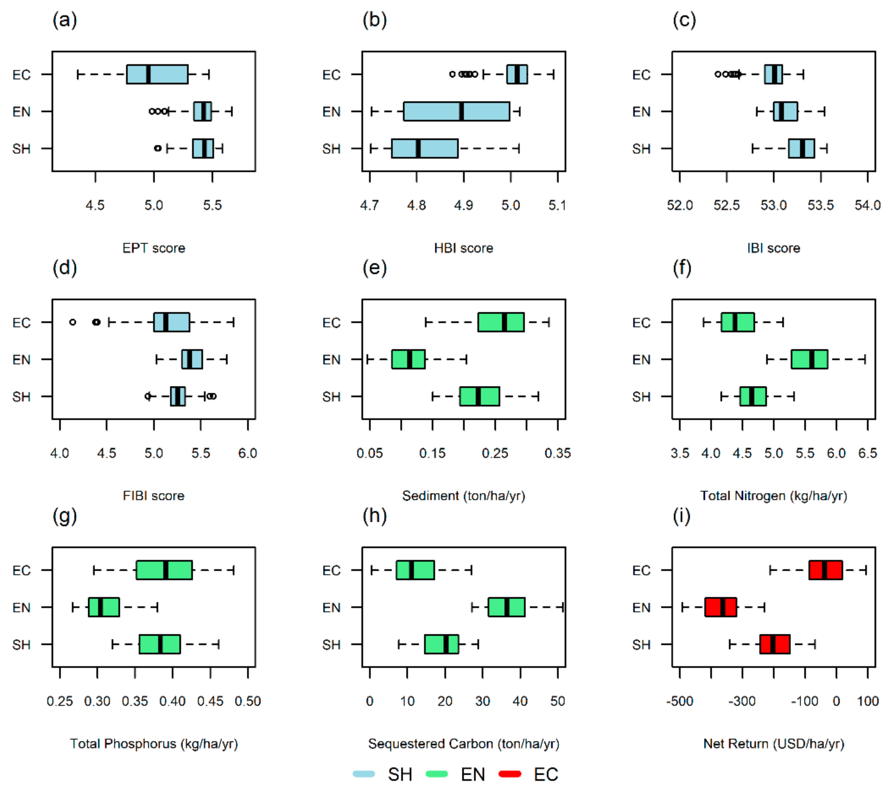
The Pareto front was further divided into three clusters showing the closeness of the Pareto-optimal solutions to each individual objective optimum (i.e., economic, environmental, and stream health). Clusters of solutions for the three objectives were generated using the k-means clustering approach, which gathers points around the mean of all points [89]. Figure 4 also shows the most-preferred solutions obtained using the compromise programming approach with equally balanced pseudo-weights, and the most balanced knee point. All these compromise solutions fall within the stream health cluster. As can be seen in Figure 4, the clusters are well distributed almost equally, with the environmental cluster consisting of 93 solutions, the stream health cluster consisting of 78 solutions, and the economic cluster consisting of 62 solutions. The solutions obtained for each cluster are further analyzed to capture their central tendency and dispersion (Figure 5). In general, the economic solutions were observed to have the highest variability, whereas the stream health was observed to have the lowest.
The stream health indicators were calculated based on hydrologic indicators (i.e., water quantity), and the median of all three clusters was observed to be within 1 point of one another for all four stream health indicators (Figure 5a–d). Therefore, the small variations in stream health indicators were expected as the change in agricultural land use from food production to bioenergy feedstock production does not significantly alter the flow regimes of the nearby rivers and streams. Concerning the best solutions for the stream health (SH) cluster, the best median values for the EPT, HBI, and IBI indicators were observed under this condition (SH) compared to the environmental (EN) and economic (EC) cluster solutions (Figure 5a–c). The only indicator that ranked second-best was the FIBI indicator, as seen in Figure 5d. The high scores from the EPT, HBI, and IBI balance out the slightly lower FIBI score given that all four values held equal weight within the optimization.
Both the median and interquartile range of the SH cluster for the four indicators were very similar to the mean and interquartile range of the EN cluster. These similarities can also be observed in the higher density of solutions in the EN and SH clusters within Figure 4 and may be explained by the lower sediment and nutrient loads to which the taxa of macroinvertebrates are highly sensitive (see Figure 5a,b) [53,90]. The EN cluster held the optimum solution for each variable besides total nitrogen, where it had the highest median load and EC cluster had the lowest (Figure 5f). This is most likely a result of the higher biomass producing crops, such as miscanthus and corn, requiring higher amounts of nitrogen inputs than legumes, which fix their own nitrogen through a symbiotic relationship with nitrogen-fixing bacteria [48]. Finally, soybeans, a legume, were observed to be the most profitable during the time period used for this study (Table S4 in Supplementary Materials), but their low biomass could explain the poor EPT, HBI, IBI, and FBI scores and higher sediment loss and nutrient loads of the EC cluster (Figure 5a–h). Crop rotations observed within the EN cluster solutions had lower sediment erosion and higher carbon sequestration than SH or EC clusters, likely due to the increased quantity of high biomass producing crops, which was also observed by Lemus and Lal [91].
3.2. Distribution of Bioenergy Feedstocks within the Watershed for Most-Preferred Trade-Off Solutions
Three most-preferred trade-off solutions from the Pareto front were determined through different methods. First, the Euclidean norm approach, was applied to identify the most-preferred trade-off solution based on the distance of the points to the origin. The pseudo-weight approach was also applied, which determined the best solution that was closest to a uniform pseudo-weight value of 1/3 for each objective [92]. Finally, the most balanced high trade-off solution was determined by finding the knee point with the most balanced pseudo-weight vector (Figure 4).
Figure 6 compares the rotation distribution of the calculated most-preferred trade-off solutions (Figure 6g–i), the preferred trade-off solutions when one of the pseudo-weights has twice the importance of any of the other two (Figure 6d–f), and the individually optimum solution for stream health (Figure 6a), environment (Figure 6b), and economy (Figure 6c). It can be observed that miscanthus was beneficial for the environment (Figure 6b), accounting for all of the agricultural land. Love and Nejadhashemi [8] also observed that significant shifts towards miscanthus production resulted in the lowest levels of total sediment and phosphorus loads. Additionally, Agostini et al. [93] observed the highest level of carbon sequestration with miscanthus among studied bioenergy crops. On the other hand, soybeans were the most profitable as represented in the optimal economic rotation distribution (Figure 6c), with the entire optimal economic watershed observed to be covered by soybeans. The stream health and all six preferred trade-off solutions represented diverse rotation distributions over the entire watershed. Even though they included varying distributions of different crops, miscanthus was commonly distributed over all scenarios, besides the optimal economic, on the south edge of the watershed.
It can be observed in Figure 6b,c,e,f that the solutions across the Pareto front varied in a distinctive pattern along the left boundary between the best environment and best economic solutions. Even though the environmentally and economically optimal solutions consisted of monocrops, the preferential environment solution was observed to have an almost equal split sorghum-soybean to miscanthus and the preference for profit was balanced with soybean, sorghum-soybean, corn-soybean, and miscanthus (Figure 6e,f). The points along the front’s boundary were observed to be interspersed with miscanthus within the environmental cluster and completed with sorghum-soybean within the economic cluster until a small void was reached (Figure 4). On one side of the void were solutions with primarily sorghum-soybean, while on the other side was primarily soybean. The sorghum-soybean rotation was therefore rated relatively highly for environmental benefits whilst also profitable in this study, which follows the observations of Sperow [94] who also observed higher soybean and sorghum carbon and economic benefit.
Similar rotation distribution patterns can be observed on the right side of the front with Figure 6a,d,g,i having corn-stover similarly placed towards the east side of the map in each of the solutions. Aside from corn-stover and miscanthus in the middle of the watershed, the optimal solutions close to the best stream health solution were observed to be quite diverse in comparison to the solutions from the left side of the front (Figure 6). Stream health scores were calculated primarily based on flow regimes as a result of previously performed sensitivity analyses [95]. Flow regimes have been observed to change the most significantly with increased urbanization or agriculture, neither of which were simulated within this study. This led to a very small margin of variation between the stream health scores and low impact of specific crop rotations on the individual stream health scores.
The solutions represented in Figure 6 shows the benefit of using multi-objective optimization in bioenergy feedstock rotation planning. The best solution for each objective (Figure 6a–c) were observed to be different than the best trade-off solutions (Figure 6d–i) with the single objective optimal solutions presenting less biodiversity than the best trade-off solutions. Our results were supported by findings showing that biological diversity is important for both ecosystem [96] and risk aversion associated with monocultures [97]. The best trade-off approach from multi-objective optimization provided solutions that were sustainable for the region through decreased negative impacts to stream health and the environment and increased economic impact, overall increasing the watershed’s sustainability and resiliency.
3.3. Comparison of Evaluation Metrics between Optimal Solutions and Current Land Use Scenario
The goal of this section of the study is to compare the differences between the individual evaluation metrics of the complete current agricultural land use to the optimized individual and most-preferred trade-off solutions. Table 1 shows the percent difference for each evaluation metric between the current agricultural practices in the watershed, the most-preferred trade-off solutions and three extreme solutions.
The current watershed agricultural makeup is 0.001% field pea, 0.004% sugar beet, 5% alfalfa, 6% winter wheat, 17% soybean, and 72% corn. Currently, only 5% of the Honeyoey Creek-Pine Creek watershed is covered by perennial crops, which can be observed by the 81% decrease in sediment load and 601% increase in carbon sequestration from the best environment solution (Table 1). Interestingly, the total nitrogen load was higher in all of the calculated optimal solutions than the reference scenario (Table 1). This could be attributed to the additional food crops grown in the watershed not considered within this study, such as alfalfa, which is a legume and maintains year-round groundcover [98]. Compared to the three best trade-off solutions, slight water quality change was observed with improvement from the EPT, HBI, and IBI indices and degradation of the FIBI score, which follows the minimum changes in stream health score also observed by Herman et al. [78]. Table 1 also shows the importance of taking multiple objectives into account when optimizing bioenergy feedstock landscape within a watershed. Both the net sequestrated carbon and net return column showed the greatest magnitude of percent change between the current and optimal solutions. The greatest net sequestrated carbon change was observed to coincide with the greatest degradation of profit of the best environment solution, while the least amount of change for both metrics coincided with the best economic solution. All of the Pareto-optimal solutions, best stream health, and best environmental solution included perennial bioenergy feedstocks (Figure 6), which currently hold a much lower market value than the other crops (Table S4 in Supplementary Materials). Glithero et al. [99] showed that in order to have the greatest carbon sequestration, high biomass perennial bioenergy feedstocks would have to significantly increase in value, which was matched with our observations within Table 1. Trade-off solutions are therefore very valuable for decision-makers when evaluating agricultural land use within a watershed in the current climate and economy.
4. Conclusions
Multi-objective optimization has been shown to be useful for applications where a decision is influenced by multiple factors. In this paper, the multi-objective optimization approach was shown to be effective in generating a set of individual optimal solutions for bioenergy feedstock production within a watershed-based on stream health, environmental, and economic criteria. Up to this point, bioenergy feedstock application has been based on satisfying only one or two objectives. Optimizing for multiple objectives ensures a solution is chosen that is sustainable for the earth, decision-makers, and economy.
To show the potential of this approach, nine trade-off solutions were determined. The first three solutions put 100% weight on each of the three objectives separately, whereas the remaining six put equal weight on all three objectives. After analyzing the rotation distribution for each of the trade-off solutions, it was noted that miscanthus had the biggest environmental impact, whereas soybean had the largest net return. In comparison, the stream health and most-preferred trade off solutions were observed to be diverse with at least nine out of ten rotations considered for application over the entire watershed.
The Pareto front was found to have discontinuities, particularly near small economic score solutions. The study revealed that contrary to general practices of optimizing a linearly weighted sum of objectives, the use of a global evolutionary multi-objective optimization has a better scope of addressing such irregularities. The best economic solutions usually exhibit non-linear properties and therefore finding a representative Pareto front by an efficient nonlinear optimization algorithm provides decision-makers a comprehensive and flexible tool for choosing a single most-preferred solution. Patterns in the front were also identified with common rotations found within each cluster. These patterns will allow decision-makers to understand the trend of rotations for specific goals for their bioenergy feedstock rotation problem.
The Pareto front contains an unbiased array of optimal solutions. In this study, we showed the benefit of using the Pareto front as a decision-making tool through selecting the most-preferred trade-off solutions based on decision-maker’s preferences. Importantly, we have also shown that due to the availability of multiple Pareto solutions, they can be analyzed to extract key insights about the common properties of them, which can stay as domain-knowledge for future applications. In addition, we demonstrated the use of other decision-making approaches to select a preferred solution from the Pareto front. One popular idea is for the decision-maker to provide an aspiration point containing three desired objective values and then identify the Pareto solution which is closest to the supplied aspiration point.
This paper showed the potential for multi-objective optimization on determining bioenergy feedstock rotations on agricultural land within a watershed. In this approach, each subbasin was assumed to apply only one bioenergy feedstock rotation over the entire area for the 12-year period. Additionally, it was assumed that all agricultural land within the watershed would be used for bioenergy feedstock production. Finally, the LCA was performed within the scope of seed to harvest rather than well-to-wheel. Further research is necessary to make this optimization more applicable to agricultural areas within the US and quantify emission savings by incorporating other factors affecting bioenergy crop expansions, such as food security and societal and political perceptions.
Supplementary Materials
The following are available online at https://www.mdpi.com/2071-1050/13/3/1424/s1, Table S1. Calibration and validation performance evaluation of SWAT simulated data against USGS station 04155500 observations [37,38,39], Table S2. Example life cycle analysis calculation of soybean crop, Table S3. Example economic analysis of soybean production USD per planted hectare in Northern Crescent U.S. [21], Table S4. Economic analysis bioenergy crop production over 12-year period in USD per hectare, Figure S1. Initial population and Pareto-optimal solutions front.
Author Contributions
A.R.: Formal analysis, Writing, Investigation; J.S.H.-S.: Writing, Software, Methodology, Visualization, Data Curation; A.P.N.: Conceptualization, Methodology, Supervision; K.D.: Review & Editing, Formal analysis. All authors have read and agreed to the published version of the manuscript.
Funding
This research was funded by the National Science Foundation under Cooperative Agreement No. DBI-0939454 and the USDA National Institute of Food and Agriculture, Hatch project 1019654.
Institutional Review Board Statement
Not applicable.
Informed Consent Statement
Not applicable.
Data Availability Statement
The data presented in this study are available on request from the corresponding author.
Acknowledgments
This material is based in part upon work supported by the National Science Foundation. However, any opinions, findings, and conclusions or recommendations expressed in this material are those of the author(s) and do not necessarily reflect the views of the National Science Foundation.
Conflicts of Interest
The authors declare no conflict of interest.
References
- U.S. EIA; Kahan, A. EIA Projects Nearly 50% Increase in World Energy Usage by 2050, Led by Growth in Asia. Today in Energy. 2019. Available online: https://www.eia.gov/todayinenergy/detail.php?id=41433 (accessed on 25 December 2020).
- United Nations. The Sustainable Development Agenda. 17 Goals to Transform Our World. 2015. Available online: https://www.un.org/sustainabledevelopment/development-agenda/ (accessed on 25 December 2020).
- IRENA. Renewable Energy Now Accounts for a Third of Global Power Capacity. 2019. Available online: https://www.irena.org/newsroom/pressreleases/2019/Apr/Renewable-Energy-Now-Accounts-for-a-Third-of-Global-Power-Capacity (accessed on 25 December 2020).
- IEA. Transport. Renewables 2019. 2019. Available online: https://www.iea.org/reports/renewables-2019/transport#abstract (accessed on 25 December 2020).
- USEPA. Overview for Renewable Fuel Standard. Renewable Fuel Standard Program. 2017. Available online: https://www.epa.gov/renewable-fuel-standard-program/overview-renewable-fuel-standard (accessed on 25 December 2020).
- Langholtz, M.; Stokes, B.; Eaton, L. 2016 billion-ton report: Advancing domestic resources for a thriving bioeconomy (Executive Summary). Ind. Biotechnol. 2016, 12, 282–289. [Google Scholar] [CrossRef]
- Bai, Y.; Dahl, C. Evaluating the management of U.S. Strategic Petroleum Reserve during oil disruptions. Energy Policy. 2018, 117, 25–38. [Google Scholar] [CrossRef]
- Love, B.J.; Nejadhashemi, A.P. Water quality impact assessment of large-scale biofuel crops expansion in agricultural regions of Michigan. Biomass Bioenergy 2011, 35, 2200–2216. [Google Scholar] [CrossRef]
- Hoekman, S.K.; Broch, A. Environmental implications of higher ethanol production and use in the U.S.: A literature review. Part II—Biodiversity, land use change, GHG emissions, and sustainability. Renew. Sustain. Energy Rev. 2018, 81, 3159–3177. [Google Scholar] [CrossRef]
- Searchinger, T.; Heimlich, R.; Houghton, R.A.; Dong, F.; Elobeid, A.; Fabiosa, J.; Tokgoz, S.; Hayes, D.; Yu, T.-H. Use of U.S. croplands for biofuels increases greenhouse gases through emissions from land-use change. Science 2008, 319, 1238–1240. [Google Scholar] [CrossRef] [PubMed]
- Nyakatawa, E.Z.; Mays, D.A.; Tolbert, V.R.; Green, T.H.; Bingham, L. Runoff, sediment, nitrogen, and phosphorus losses from agricultural land converted to sweetgum and switchgrass bioenergy feedstock production in north Alabama. Biomass Bioenergy 2006, 30, 655–664. [Google Scholar] [CrossRef]
- Lal, R. Restoring Soil Quality to Mitigate Soil Degradation. Sustainability 2015, 7, 5875–5895. [Google Scholar] [CrossRef] [Green Version]
- Bot, A.; Benites, J. Practices that Influence the Amount of Organic Matter. The Importance of Soil Organic Matter. Food and Agriculture Organization of the United Nations. 2005. Available online: http://www.fao.org/3/a0100e/a0100e00.htm#Contents (accessed on 25 December 2020).
- Jacobson, P.C.; Hansen, G.J.A.; Bethke, B.J.; Cross, T.K. Disentangling the effects of a century of eutrophication and climate warming on freshwater lake fish assemblages. PLoS ONE 2017, 12, e0182667. [Google Scholar] [CrossRef] [Green Version]
- Rowe, H.; Withers, P.J.A.; Baas, P.; Chan, N.I.; Doody, D.; Holiman, J.; Jacobs, B.; Li, H.; MacDonald, G.K.; McDowell, R.; et al. Integrating legacy soil phosphorus into sustainable nutrient management strategies for future food, bioenergy and water security. Nutr. Cycl. Agroecosystems 2016, 104, 393–412. [Google Scholar] [CrossRef]
- Kirchmann, H.; Johnston, A.E.J.; Bergström, L.F. Possibilities for Reducing Nitrate Leaching from Agricultural Land. AMBIO A J. Hum. Environ. 2002, 31, 404–408. [Google Scholar] [CrossRef]
- U.S. EIA. Where Greenhouse Gases Come from. Energy and the Environment Explained. 2020. Available online: https://www.eia.gov/energyexplained/energy-and-the-environment/where-greenhouse-gases-come-from.php (accessed on 25 December 2020).
- Chillrud, R. Biofuels versus Gasoline: The Emissions Gap is Widening. Environmental and Energy Study Institute. 2016. Available online: https://advancedbiofuelsusa.info/biofuels-versus-gasoline-the-emissions-gap-is-widening/Contents (accessed on 25 December 2020).
- Follett, R.F.; Vogel, K.P.; Varvel, G.E.; Mitchell, R.B.; Kimble, J. Soil Carbon Sequestration by Switchgrass and No-Till Maize Grown for Bioenergy. Bioenergy Res. 2012, 5, 866–875. [Google Scholar] [CrossRef] [Green Version]
- MSU Product Center; Shepherd Advisors. Michigan’s Position in the U.S. Biofuel and Bioenergy Market. 2010. Available online: https://www.canr.msu.edu/productcenter/uploads/files/michiganspositionintheusbiofuelandbioenergymarket.pdf (accessed on 25 December 2020).
- USDA ERS. U.S. Bioenergy Statistics. 2020. Available online: https://www.ers.usda.gov/data-products/us-bioenergy-statistics/us-bioenergy-statistics/#Feedstocks (accessed on 25 December 2020).
- Amoah, J.; Kahar, P.; Ogino, C.; Kondo, A. Bioenergy and Biorefinery: Feedstock, Biotechnological Conversion, and Products. Biotechnol. J. 2019, 14, 1800494. [Google Scholar] [CrossRef] [PubMed]
- FAO. Perennial Agriculture: Landscape Resilience for the Future Do We Need to Shift Agriculture and Transform Cropping Systems? 2011. Available online: http://www.fao.org/fileadmin/templates/agphome/documents/scpi/PerennialPolicyBrief.pdf (accessed on 25 December 2020).
- Dale, B.E.; Holtzapple, M. The need for biofuels. Chem. Eng. Prog. 2015, 111, 36–40. [Google Scholar]
- Giri, S.; Nejadhashemi, A.P.; Woznicki, S.A. Regulators’ and stakeholders’ perspectives in a framework for bioenergy development. Land Use Policy 2016, 59, 143–153. [Google Scholar] [CrossRef] [Green Version]
- Lee, M.-S.; Mitchell, R.; Heaton, E.; Zumpf, C.; Lee, D.K. Warm-Season Grass Monocultures and Mixtures for Sustainable Bioenergy Feedstock Production in the Midwest, USA. Bioenergy Res. 2019, 12, 43–54. [Google Scholar] [CrossRef] [Green Version]
- Mitchell, R.B.; Schmer, M.R.; Anderson, W.F.; Jin, V.; Balkcom, K.S.; Kiniry, J.; Coffin, A.; White, P. Dedicated Energy Crops and Crop Residues for Bioenergy Feedstocks in the Central and Eastern USA. Bioenergy Res. 2016, 9, 384–398. [Google Scholar] [CrossRef] [Green Version]
- USEPA. Saginaw River and Bay AOC. Great Lakes AOCs. 2020. Available online: https://www.epa.gov/great-lakes-aocs/saginaw-river-and-bay-aoc#restoration (accessed on 25 December 2020).
- Pennington, D.; Gould, M.C.; Seamon, M.; Knudson, W.; Gross, P.; McLean, T. Expanding Bioenergy Crops to Non-Traditional Lands in Michigan: Final Report. 2012. Available online: http://msue.anr.msu.edu/uploads/files/F2F/DELEGdraftreport04-03-2012Final.pdf (accessed on 25 December 2020).
- Arnold, J.G.; Moriasi, D.N.; Gassman, P.W.; Abbaspour, K.C.; White, M.J.; Srinivasan, R.; Santhi, C.; Harmel, R.D.; van Griensven, A.; Van Liew, M.W.; et al. SWAT: Model Use, Calibration, and Validation. Trans. Asabe 2012, 55, 1491–1508. [Google Scholar] [CrossRef]
- Gassman, P.W.; Sadeghi, A.M.; Srinivasan, R. Applications of the SWAT Model Special Section: Overview and Insights. J. Environ. Qual. 2014, 43, 1–8. [Google Scholar] [CrossRef]
- Delkash, M.; Al-Faraj, F.A.M.; Scholz, M. Impacts of Anthropogenic Land Use Changes on Nutrient Concentrations in Surface Waterbodies: A Review. Clean SoilAirWater 2018, 46, 1800051. [Google Scholar] [CrossRef] [Green Version]
- Neitsch, S.L.; Arnold, J.G.; Kiniry, J.R.; Williams, J.R. Soil and Water Assessment Tool Theoretical Documentation Version 2009; Texas Water Resources Institute: College Station, TX, USA, 2011. [Google Scholar]
- USGS. The National Map. National Geopacial Program. 2020. Available online: https://www.usgs.gov/core-science-systems/national-geospatial-program/national-map (accessed on 25 December 2020).
- Soil Survey Staff, Web Soil Survey. 2020. Available online: https://websoilsurvey.nrcs.usda.gov/ (accessed on 25 December 2020).
- USDA. CropScape—Cropland Data Layer. National Agricultural Statistics Services. 2020. Available online: https://nassgeodata.gmu.edu/CropScape/ (accessed on 25 December 2020).
- NCDC. Climate Data Online. 2020. Available online: https://www.ncdc.noaa.gov/cdo-web/datatools/findstation (accessed on 25 December 2020).
- Moriasi, D.N.; Arnold, J.G.; Liew, M.W.; Van Bingner, R.L.; Harmel, R.D.; Veith, T.L. Model Evaluation Guidelines for Systematic Quantification of Accuracy in Watershed Simulations. Trans. Asabe 2007, 50, 885–900. [Google Scholar] [CrossRef]
- Gupta, H.V.; Kling, H.; Yilmaz, K.K.; Martinez, G.F. Decomposition of the mean squared error and NSE performance criteria: Implications for improving hydrological modelling. J. Hydrol. 2009, 377, 80–91. [Google Scholar] [CrossRef] [Green Version]
- Kling, H.; Fuchs, M.; Paulin, M. Runoff conditions in the upper Danube basin under an ensemble of climate change scenarios. J. Hydrol. 2012, 424–425, 264–277. [Google Scholar] [CrossRef]
- Daneshvar, F.; Nejadhashemi, A.P.; Herman, M.R.; Abouali, M. Response of benthic macroinvertebrate communities to climate change. Ecohydrol. Hydrobiol. 2017, 17, 63–72. [Google Scholar] [CrossRef] [Green Version]
- Glavan, M.; Pintar, M. Strengths, Weaknesses, Opportunities and Threats of Catchment Modelling with Soil and Water Assessment Tool (SWAT) Model. Water Res. Manag. Model. 2012, 39–64. [Google Scholar]
- Battel, R. Site-Specific Corn Nitrogen Management. MSU Extension Corn. 2018. Available online: https://www.canr.msu.edu/news/site-specific-corn-nitrogen-management (accessed on 25 December 2020).
- Min, D.H. Getting your N Application Correct can Boost Switchgrass Production—MSU Extension. MSU Extension. 2012. Available online: https://www.canr.msu.edu/news/switchgrass_nitrogen_fertility_study (accessed on 25 December 2020).
- Staton, M. Nutrient Management Recommendations for Profitable Soybean Production. MSU Extension. 2018. Available online: https://www.canr.msu.edu/news/nutrient_management_recommendations_for_profitable_soybean_production (accessed on 25 December 2020).
- Thelen, K.D.; Gao, J.; Hoben, J.; Qian, L.; Saffron, C.; Withers, K. A spreadsheet-based model for teaching the agronomic, economic, and environmental aspects of bioenergy cropping systems. Comput. Electron. Agric. 2012, 85, 157–163. [Google Scholar] [CrossRef]
- Pennington, D.; Jean, M.; Thelen, K.; Rust, S.; Anderson, E.; Gould, K. Michigan Corn Stover Project: Cattle, Storage and Bioenergy. 2017. Available online: https://www.canr.msu.edu/corn/uploads/files/E-3354WCAG2.0.pdf (accessed on 25 December 2020).
- Vitosh, M.L.; Johnson, J.W.; Mengel, D.B. Tri-state Fertilizer Recommendations for Corn, Soybeans, Wheat and Alfalfa. Extension Bulletin. 1995. Available online: https://www.extension.purdue.edu/extmedia/AY/AY-9-32.pdf (accessed on 25 December 2020).
- Staton, M. Phosphorus and Potassium Fertilizer Recommendations for High-Yielding, Profitable Soybeans. MSU Extension. 2014. Available online: https://www.canr.msu.edu/news/phosphorus_and_potassium_fertilizer_recommendations_for_high_yielding_profi (accessed on 25 December 2020).
- MSU Extension. Canola Production in Michigan. Ext. Bull. 2001, E-2766. [Google Scholar]
- Undersander, D. Sorghums, Sudangrasses, and Sorghum-Sudan Hybrids. Focus Forage 2003, 5, 5. [Google Scholar]
- Hernandez-Suarez, J.S.; Nejadhashemi, A.P. A review of macroinvertebrate-and fish-based stream health modelling techniques. Ecohydrology 2018, 11, e2022. [Google Scholar] [CrossRef]
- Sanchez, G.M.; Nejadhashemi, A.P.; Zhang, Z.; Marquart-Pyatt, S.; Habron, G.; Shortridge, A. Linking watershed-scale stream health and socioeconomic indicators with spatial clustering and structural equation modeling. Environ. Model. Softw. 2015, 70, 113–127. [Google Scholar] [CrossRef]
- Woznicki, S.A.; Nejadhashemi, A.P.; Abouali, M.; Herman, M.R.; Esfahanian, E.; Hamaamin, Y.A.; Zhang, Z. Ecohydrological modeling for large-scale environmental impact assessment. Sci. Total Environ. 2016, 543, 274–286. [Google Scholar] [CrossRef]
- Jang, J.R. ANFIS: Adaptive-Network-Based Fuzzy Inference System. IEEE Trans. Syst. Man Cybern. 1993, 23, 665–685. [Google Scholar] [CrossRef]
- Abouali, M.; Nejadhashemi, A.P.; Daneshvar, F.; Woznicki, S.A. Two-phase approach to improve stream health modeling. Ecol. Inform. 2016, 34, 13–21. [Google Scholar] [CrossRef]
- Seifi, A.; Riahi-Madvar, H. Improving one-dimensional pollution dispersion modeling in rivers using ANFIS and ANN-based GA optimized models. Environ. Sci. Pollut. Res. 2019, 26, 867–885. [Google Scholar] [CrossRef] [PubMed]
- Poff, N.L.; Allan, J.D.; Bain, M.B.; Karr, J.R.; Prestegaard, K.L.; Richter, B.D.; Sparks, R.E.; Stromberg, J.C. The natural flow regime: A paradigm for river conservation and restoration. BioScience 1997, 47, 769–785. [Google Scholar] [CrossRef]
- Einheuser, M.D.; Nejadhashemi, A.P.; Wang, L.; Sowa, S.P.; Woznicki, S.A. Linking biological integrity and watershed models to assess the impacts of historical land use and climate changes on stream health. Environ. Manag. 2013, 51, 1147–1163. [Google Scholar] [CrossRef]
- Einheuser, M.D.; Nejadhashemi, A.P.; Sowa, S.P.; Wang, L.; Hamaamin, Y.A.; Woznicki, S.A. Modeling the effects of conservation practices on stream health. Sci. Total Environ. 2012, 435–436, 380–391. [Google Scholar] [CrossRef]
- Akamagwuna, F.C.; Mensah, P.K.; Nnadozie, C.F.; Odume, O.N. Evaluating the responses of taxa in the orders Ephemeroptera, Plecoptera and Trichoptera (EPT) to sediment stress in the Tsitsa River and its tributaries, Eastern Cape, South Africa. Environ. Monit. Assess. 2019, 191, 663–678. [Google Scholar] [CrossRef]
- Herman, M.R.; Nejadhashemi, A.P. A review of macroinvertebrate- and fish-based stream health indices. Ecohydrol. Hydrobiol. 2015, 15, 53–67. [Google Scholar] [CrossRef] [Green Version]
- Torres-Olvera, M.J.; Durán-Rodríguez, O.Y.; Torres-García, U.; Pineda-López, R.; Ramírez-Herrejón, J.P. Validation of an index of biological integrity based on aquatic macroinvertebrates assemblages in two subtropical basins of central Mexico. Lat. Am. J. Aquat. Res. 2018, 46, 945–960. [Google Scholar] [CrossRef]
- Gellings, C.W.; Paramenter, K.E. Energy efficiency in fertilizer production and use. Encycl. Life Support. Syst. 2004. [Google Scholar]
- Helsel, Z.R. Energy and alternatives for fertilizer and pesticide use. Energy Farm Prod. 1992, 6, 177–201. [Google Scholar]
- Robertson, G.P.; Paul, E.A.; Harwood, R.R. Greenhouse gases in intensive agriculture: Contributions of individual gases to the radiative forcing of the atmosphere. Science 2000, 289, 1922–1925. [Google Scholar] [CrossRef] [PubMed] [Green Version]
- Gelfand, I.; Snapp, S.S.; Robertson, G.P. Energy Efficiency of Conventional, Organic, and Alternative Cropping Systems for Food and Fuel at a Site in the U.S. Midwest. Environ. Sci. Technol. 2010, 44, 4006–4011. [Google Scholar] [CrossRef] [PubMed]
- USDOE. Bioenergy Conversion Factors; Oak Ridge National Lab.: Oak Ridge, TN, USA, 2010. [Google Scholar]
- Battel, B.; Stein, D. 2018 Custom Machine and Work Rate Estimates. Michigan State University Extension. 2018. Available online: https://www.canr.msu.edu/field_crops/uploads/files/2018%20Custom%20Machine%20Work%20Rates.pdf (accessed on 25 December 2020).
- USDA, Michigan Agricultural Statistics 2013–2014. 2013. Available online: www.nass.usda.gov (accessed on 25 December 2020).
- Smith, P. Soil organic carbon dynamics and land-use change. In Land Use and Soil Resources; Springer: Amsterdan, The Netherlands, 2008; pp. 9–22. [Google Scholar]
- Wardynski, F. Sorghum Species Crops as a Drought Emergency Crop. MSU Extension. 2012. Available online: https://www.canr.msu.edu/news/sorghum_species_crops_as_a_drought_emergency_crop (accessed on 25 December 2020).
- USDA ERS. Commodity Costs and Returns. 2020. Available online: https://www.ers.usda.gov/data-products/commodity-costs-and-returns/ (accessed on 25 December 2020).
- Pennington, D. Making Bioenergy Crops Pay. MSU Extension. 2011. Available online: https://www.canr.msu.edu/news/making_bioenergy_crops_pay (accessed on 25 December 2020).
- USDA ERS. U.S. Farm Resource Regions. In Resource Regions; Briefing Rooms ARMS: Malham, UK, 2010. [Google Scholar]
- Canola Council of Canada. Canadian Canola Yield. 2019. Available online: https://www.canolacouncil.org/markets-stats/ (accessed on 25 December 2020).
- Smith, S.A.; Bowling, B.; Buntin, R.; Williams, B.; Manning, D. Field Crop Budgets For 2014. The University of Tennessee, Institute of Agriculture. 2014. Available online: https://ag.tennessee.edu/arec/Documents/budgets/archived/2014RowCropBudgets.pdf (accessed on 25 December 2020).
- Herman, M.R.; Nejadhashemi, A.P.; Daneshvar, F.; Abouali, M.; Ross, D.M.; Woznicki, S.A.; Zhang, Z. Optimization of bioenergy crop selection and placement based on a stream health indicator using an evolutionary algorithm. J. Environ. Manag. 2016, 181, 413–424. [Google Scholar] [CrossRef] [PubMed] [Green Version]
- Seada, H.; Deb, K. A unified evolutionary optimization procedure for single, multiple, and many objectives. IEEE Trans. Evol. Comput. 2015, 20, 358–369. [Google Scholar] [CrossRef]
- Deb, K.; Jain, H. An evolutionary many-objective optimization algorithm using reference-point-based nondominated sorting approach, part I: Solving problems with box constraints. IEEE Trans. Evol. Comput. 2014, 18, 577–601. [Google Scholar] [CrossRef]
- Hernandez-Suarez, J.S.; Nejadhashemi, A.P.; Kropp, I.M.; Abouali, M.; Zhang, Z.; Deb, K. Evaluation of the impacts of hydrologic model calibration methods on predictability of ecologically-relevant hydrologic indices. J. Hydrol. 2018, 564, 758–772. [Google Scholar] [CrossRef]
- Kropp, I.; Nejadhashemi, A.P.; Deb, K.; Abouali, M.; Roy, P.C.; Adhikari, U.; Hoogenboom, G. A multi-objective approach to water and nutrient efficiency for sustainable agricultural intensification. Agric. Syst. 2019, 173, 289–302. [Google Scholar] [CrossRef]
- Herman, M.R.; Hernandez-Suarez, J.S.; Nejadhashemi, A.P.; Kropp, I.; Sadeghi, A.M. Evaluation of multi- and many-objective optimization techniques to improve the performance of a hydrologic model using evapotranspiration remote-sensing data. J. Hydrol. Eng. 2020, 25, 1–15. [Google Scholar] [CrossRef]
- Blank, J.; Deb, K. pymoo: Multi-objective Optimization in Python. IEEE Access 2020, 8, 89497–89509. [Google Scholar] [CrossRef]
- Auger, A.; Bader, J.; Brockhoff, D.; Zitzler, E. Hypervolume-based multiobjective optimization: Theoretical foundations and practical implications. Theor. Comput. Sci. 2012, 425, 75–103. [Google Scholar] [CrossRef]
- Zeleny, M.; Cochrane, J.L. Multiple Criteria Decisions Making; University of South Carolina Press: Columbia, SC, USA, 1973. [Google Scholar]
- Deb, K. Multi-Objective Optimization Using Evolutionary Algorithms; John Wiley & Sons, Inc.: New York, NY, USA, 2001; ISBN 047187339X. [Google Scholar]
- Rachmawati, L.; Srinivasan, D. Multiobjective evolutionary algorithm with controllable focus on the knees of the Pareto front. IEEE Trans. Evol. Comput. 2009, 13, 810–824. [Google Scholar] [CrossRef]
- Vassilvitskii, A.; Vassilvitskii, D.; Vassilvitskii, S. No k-means++: The advantages of careful seeding. In Proceedings of the Eighteenth Annual ACM-SIAM Symposium on Discrete Algorithms, Society for Indistrial and Applied Mathematics, New Orleans, LA, USA, 7–9 January 2007; pp. 1027–1035. [Google Scholar]
- NRCS. The EPT Index. 2012. Available online: https://www.wcc.nrcs.usda.gov/ftpref/wntsc/strmRest/wshedCondition/EPTIndex.pdf (accessed on 25 December 2020).
- Lemus, R.; Lal, R. Bioenergy Crops and Carbon Sequestration. Crit. Rev. Plant. Sci. 2005, 24, 1–21. [Google Scholar] [CrossRef]
- Elliott, M.R. Combining Data from Probability and Non- Probability Samples Using Pseudo-Weights. Surv. Pract. 2009, 2, 1–7. [Google Scholar] [CrossRef]
- Agostini, F.; Gregory, A.S.; Richter, G.M. Carbon Sequestration by Perennial Energy Crops: Is the Jury Still Out? Bioenergy Res. 2015, 8, 1057–1080. [Google Scholar] [CrossRef] [Green Version]
- Sperow, M. The marginal costs of carbon sequestration: Implications of one greenhouse gas mitigation activity. J. Soil Water Conserv. 2007, 62, 367–375. [Google Scholar]
- Woznicki, S.A.; Nejadhashemi, A.P.; Ross, D.M.; Zhang, Z.; Wang, L.; Esfahanian, A.H. Ecohydrological model parameter selection for stream health evaluation. Sci. Total Environ. 2015, 511, 341–353. [Google Scholar] [CrossRef]
- COP. Agricultural biological diversity. Secretariat of the Convention on Biological Diversity. 2000. Available online: https://www.cbd.int/decision/cop/?id=7147 (accessed on 25 December 2020).
- FAO. Agricultural Practices to Manage Agricultural Biodiversity. How to Manage Biodiversity for Food and Agriculture. 2020. Available online: http://www.fao.org/agriculture/crops/thematic-sitemap/theme/spi/scpi-home/managing-ecosystems/biodiversity-and-ecosystem-services/bio-how/en/ (accessed on 25 December 2020).
- Department of Plant Sciences University of Wyoming. Forage Identification: Alfalfa. 2020. Available online: http://www.uwyo.edu/plantsciences/uwplant/forages/legume/alfalfa.html (accessed on 25 December 2020).
- Glithero, N.J.; Ramsden, S.J.; Wilson, P. Farm systems assessment of bioenergy feedstock production: Integrating bio-economic models and life cycle analysis approaches. Agric. Syst. 2012, 109, 53–64. [Google Scholar]
Figure 1.
Honeyoey Creek-Pine Creek watershed within the Saginaw River watershed in Michigan, U.S.
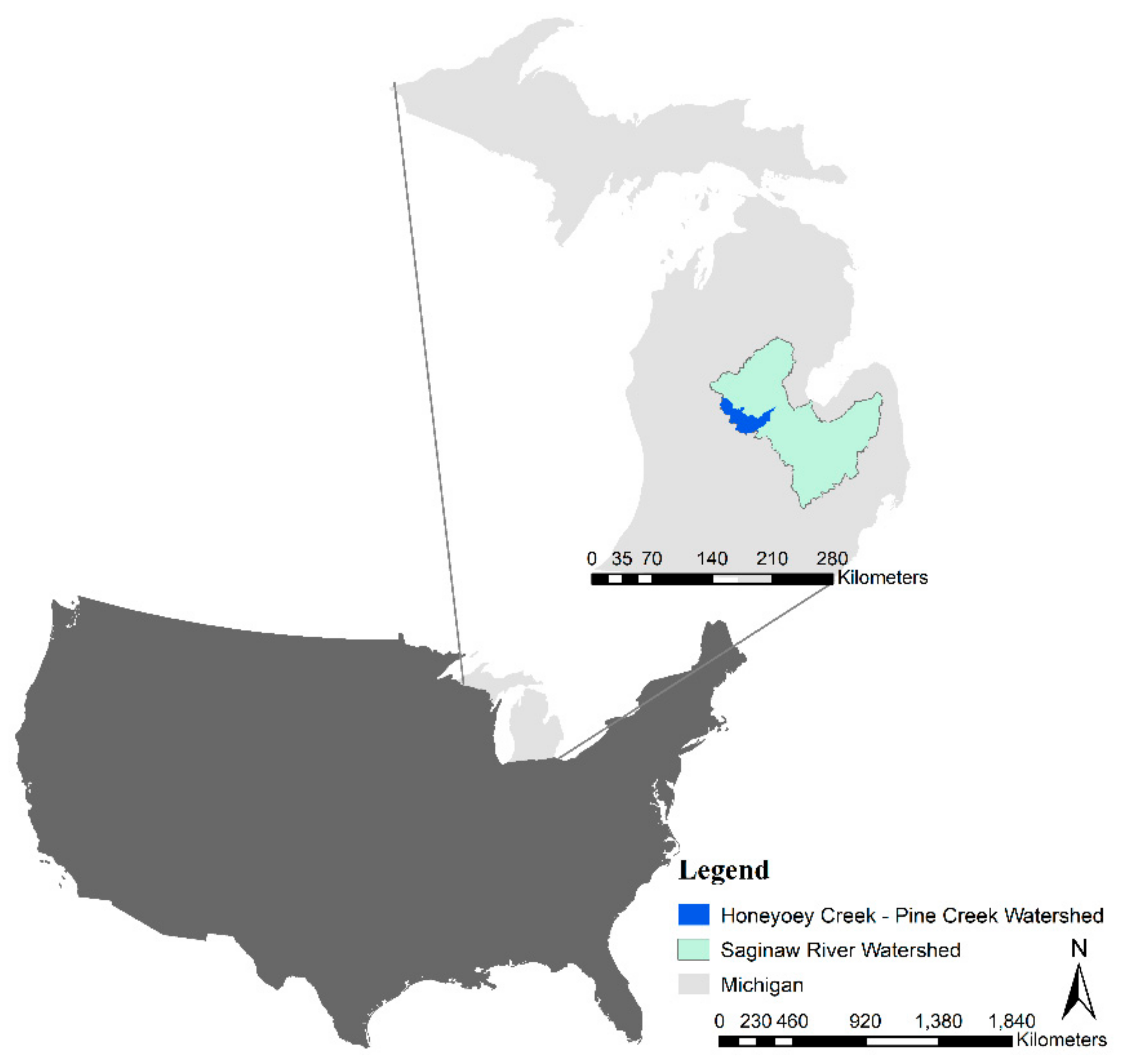
Figure 2.
A schematic diagram presenting the overall multi-objective optimization framework for the selection and placement of biofuel crops.
Figure 2.
A schematic diagram presenting the overall multi-objective optimization framework for the selection and placement of biofuel crops.

Figure 3.
Hypervolume indicator and number of Pareto-optimal points at the end of each Unified Non-Dominated Sorting Genetic Algorithm III (U-NSGA-III) generation.
Figure 3.
Hypervolume indicator and number of Pareto-optimal points at the end of each Unified Non-Dominated Sorting Genetic Algorithm III (U-NSGA-III) generation.

Figure 4.
Clustered optimal Pareto front based on normalized economic, environmental, and stream health scores and most-preferred solutions.
Figure 4.
Clustered optimal Pareto front based on normalized economic, environmental, and stream health scores and most-preferred solutions.

Figure 5.
Cluster variable distribution with focuses on stream health (SH), environmental (EN), and economic (EC) central tendency and dispersion.
Figure 5.
Cluster variable distribution with focuses on stream health (SH), environmental (EN), and economic (EC) central tendency and dispersion.

Figure 6.
Relevant Pareto-optimal solutions: (a) best solution in terms of stream health, (b) best solution in terms of environment, (c) best solution in terms of net return, (d) trade-off solution with preference for stream health, (e) trade-off solution with preference for the environment, (f) trade-off solution with preference for net return, (g) most-preferred trade-off solution by compromise programming using the metric (Euclidian distance), (h) most-preferred trade-off solution selecting the most balanced pseudo-weight, and (i) most balanced high trade-off solution.


Table 1.
Percent change between evaluation metrics of select optimal solutions to current agriculture on an annual per hectare basis.
Table 1.
Percent change between evaluation metrics of select optimal solutions to current agriculture on an annual per hectare basis.
| Solution | EPT | HBI | IBI | FIBI | Total Sediment | Total Nitrogen | Total Phosphorus | Net Sequestrated C | Net Return |
|---|---|---|---|---|---|---|---|---|---|
| Compromise programming | 9% | −1% | 2% | 0% | −33% | 96% | −12% | 293% | −583% |
| Balanced Pseudo-weights | 4% | −1% | 1% | −1% | −29% | 88% | −16% | 244% | −463% |
| Most balanced high trade-off | 10% | −3% | 2% | −2% | −1% | 64% | 1% | 99% | −362% |
| Best stream health | 10% | −6% | 3% | 2% | 13% | 71% | 8% | 198% | −658% |
| Best environment | 7% | −1% | 2% | 6% | −81% | 137% | −30% | 601% | −1064% |
| Best economic | −14% | 1% | 1% | −6% | 32% | 67% | 15% | −30% | 86% |
Publisher’s Note: MDPI stays neutral with regard to jurisdictional claims in published maps and institutional affiliations. |
© 2021 by the authors. Licensee MDPI, Basel, Switzerland. This article is an open access article distributed under the terms and conditions of the Creative Commons Attribution (CC BY) license (http://creativecommons.org/licenses/by/4.0/).
Share and Cite
MDPI and ACS Style
Raschke, A.; Hernandez-Suarez, J.S.; Nejadhashemi, A.P.; Deb, K. Multidimensional Aspects of Sustainable Biofuel Feedstock Production. Sustainability 2021, 13, 1424. https://doi.org/10.3390/su13031424
AMA Style
Raschke A, Hernandez-Suarez JS, Nejadhashemi AP, Deb K. Multidimensional Aspects of Sustainable Biofuel Feedstock Production. Sustainability. 2021; 13(3):1424. https://doi.org/10.3390/su13031424
Chicago/Turabian StyleRaschke, Anna, J. Sebastian Hernandez-Suarez, A. Pouyan Nejadhashemi, and Kalyanmoy Deb. 2021. "Multidimensional Aspects of Sustainable Biofuel Feedstock Production" Sustainability 13, no. 3: 1424. https://doi.org/10.3390/su13031424
Note that from the first issue of 2016, this journal uses article numbers instead of page numbers. See further details here.