Article

Multi-Objective Optimization of Back-to-Back Starting for Pumped Storage Plants under Low Water Head Conditions Based on the Refined Model

1
College of Energy and Electrical Engineering, Hohai University, Nanjing 211100, China
2
Department of Rural Water Management, Nanjing Hydraulic Research Institute, Nanjing 210029, China
*
Author to whom correspondence should be addressed.
Sustainability 2022, 14(16), 10289; https://doi.org/10.3390/su141610289
Submission received: 19 July 2022 / Revised: 13 August 2022 / Accepted: 15 August 2022 / Published: 18 August 2022
(This article belongs to the Special Issue Ocean and Hydropower)

Abstract

:
Pumped storage plants (PSP) must switch frequently between various working conditions. Moreover, PSPs can fall easily into an S-shaped zone under low water head conditions, especially during back-to-back starting (BTBS), which reduces the stability and safety of unit operation. In this paper, a nonlinear PSP model for BTBS is established by combining an electrical subsystem with a refined hydraulic-mechanical subsystem. The influences of the hydraulic, mechanical, and electrical factors on the BTBS process are investigated quantitatively. Choosing the speed overshoot and speed stable time as the optimization objectives, and considering a variety of constraints, the multi-objective particle swarm optimization (MOPSO) algorithm is introduced to study and optimize two typical startup strategies. The results show that: (1) The parameters of a hydraulic-mechanical-electrical system have a significant impact on BTBS process, and the most unfavorable working condition corresponds to the lowest water head; (2) In the control schemes, a novel constant excitation voltage strategy is proposed based on the multi-objective optimization scheme. Compared with the constant excitation current strategy or single-objective, the optimization strategy proposed can considerably improve the speed overshoot and the speed stable time by at least 68.27% and 3.22% under the worst working conditions. (3) It is further verified that the problem of trapping in the S-shaped region under various working conditions may be avoided by the obtained optimal control scheme. The results give prominence to the effectiveness of the proposed optimization strategy for maintaining the safety and stabilization of PSP operation.

1. Introduction

In order to cope with climate change, many renewable energy sources have been developed, such as tidal, wind, solar, and hydro energies [1]. As unstable renewable energy is connected to the grid in large quantities and the load demand is diversified, the power grid’s supply and demand fluctuation is becoming more serious [2,3]. As an essential energy storage technology, a pumped storage plant (PSP) can effectively adjust the impact of unstable energy on the power system and enhance the consumption capacity of the power grid for unstable energy such as solar energy and wind power [4,5]. However, during the large fluctuation transition process of the pumped storage unit (PSU), due to the influence of the S-shaped curve of the pump turbine, the water hammer effect in the penstock of the diversion system causes an effect similar to the rapid closing of guide vanes, and the inflow decreases rapidly, resulting in the sharp rise of water pressure and speed, threatening the structural safety of unit and diversion pipelines [6,7]. The above operation characteristics and various potential operation accidents not only seriously endanger the safe and stable operation of PSPs, but also affect the safety and stability of the power supplies.
At present, the conventional startup mode of large PSPs at home and abroad is mainly via a static frequency converter starting and BTBS as standby [8,9,10]. During variable frequency starting, it is necessary to absorb electric energy from the power grid. If the power grid or the frequency converter fails, the unit cannot be started in this way, but the BTBS mode can meet the requirements well. Therefore, the experience and technology of BTBS should be explored in the context of building a resilient power grid. Among the numerous startup conditions of the PSU, the BTBS mode is the most complicated, requiring the mutual cooperation of monitoring, speed regulation, excitation, protection, and other systems of the two units, which presents an enormous challenge to the stable operation of PSPs. However, this issue has not been fully addressed until now. Previous studies have mainly focused on the transient electrical characteristics and electromechanical variation law. Relevant research findings are summarized as follows:
For BTBS modelling, previous studies focus on the electrical perspective by greatly simplifying the hydraulic and mechanical systems. The functions offered by turbine manufacturers and obtained by model tests, which are used to describe the dynamic behaviors among the mechanical torque, gate valve opening (GVO), and speed, have been widely adopted [11,12]. However, these models are mostly oversimplified based on strong assumptions in reflecting the coupling characteristics of the hydraulic-mechanical-electrical subsystems of a PSP under various working conditions, especially the S-shaped characteristics under low head conditions. Therefore, a nonlinear model with a detailed hydraulic-mechanical system, i.e., the logarithmic curve projection (LCP) method for pump turbine [13], and the method of characteristics (MOC) for conduit systems [14], has been adopted to improve the accuracy of the BTBS transient processes simulation in this work, which can overcome the shortcomings of the above-simplified models.
For analysis of influencing factors, Konidaris [12] systematically discussed the main parameters’ impact on the performance of the BTBS based on the physical laws behind the transient process. Osburn and Atwater [15] described the design and testing of a BTBS system. The feasibility of this kind of startup is analyzed theoretically. Guidance was developed in order to correctly select the main parameters for a successful start [16]. By means of simulating the transient starting performance for a PSU, alternative designs and their effects on the startup ability of the PSU for reliable improvement of the starting system were studied [17]. Proposals were offered to achieve safe and reliable fault clearance on the basis of the fault characteristics and actual deexcitation test results of the PSP [18].
For control optimization, there are many applications of the MOPSO algorithm in energy systems; A. Beiranvand applied the MOPSO algorithm in the optimization analysis of thermal power generation [19], and M. Ghazvini proposed the Coupled Multi-Objective Evolutionary Approaches [20]. There are also multi-objective optimization cases in the field of materials and chemicals [21,22], which give some inspiration to this paper. However, the BTBS model is more complicated. There exists no report on the optimization of the BTBS control scheme, and only some research on the startup strategy of PSPs under turbine conditions has been involved. Xu et al. [23] studied the optimal control for the turbine startup process of PSPs under low head conditions. There are hydraulic, mechanical, and electrical interferences between two units, and more control factors must be taken into account during the BTBS process. Moreover, BTBS generally happens during the low power consumption period, and the upper-reservoir water storage has been exhausted during the peak power consumption period. Thus, the PSU can more easily be under low water head conditions and fall into the S-shaped zone.
Through reviews of relevant works, it was found that too little work has been devoted to BTBS in the previous research, which mainly focused on the BTBS workflow or the influence of electrical factors on the transient process of BTBS. Many other factors, such as effects from the S-shaped characteristics, are likely to affect the transient processes of BTBS and have not been studied. In addition, to our best knowledge, the control scheme optimization strategy for BTBS has not been proposed in previous works.
Accordingly, in this paper, the effect mechanisms of the hydraulic-mechanical-electrical coupling factors on BTBS are investigated, and the optimization strategy for BTBS control at low water head conditions is proposed. A nonlinear model for PSP by incorporating an electrical subsystem with a refined hydraulic-mechanical subsystem is established to conduct the study, and the effects of the electrical and hydraulic-mechanical subsystems on the process of BTBS are quantitatively investigated subsequently. Moreover, on the basis of the analysis of the influencing factors, a novel multiobjective optimization scheme for the BTBS control strategy is proposed. The innovations of this paper are as follows.
(1)
It is the first to establish a nonlinear PSP model combining the electrical subsystem with the fine hydraulic and mechanical subsystems for BTBS;
(2)
The effects of the hydraulic-mechanical-electrical parameters on the BTBS are comprehensively investigated on the basis of the model mentioned above;
(3)
An innovative multi-objective optimization scheme is proposed for the control strategy of BTBS at low water head conditions for the first time, which is proven to be suitable for a variety of working conditions.
The remainder of the paper proceeds as follows: The nonlinear model of a PSP with a refined hydraulic-mechanical subsystem is constructed and validated in Section 2. In Section 3, the effects of the hydraulic-mechanical-electrical parameters on the BTBS processes are then studied. In Section 4, an innovative multi-objective optimization scheme for BTBS in the condition of low head is proposed on the basis of the analysis above. In Section 5, a case study is conducted and the optimization result is also authenticated in other working conditions. In Section 6, the conclusions of these analyses are brought forth. Figure 1 presents the flowchart of this research.

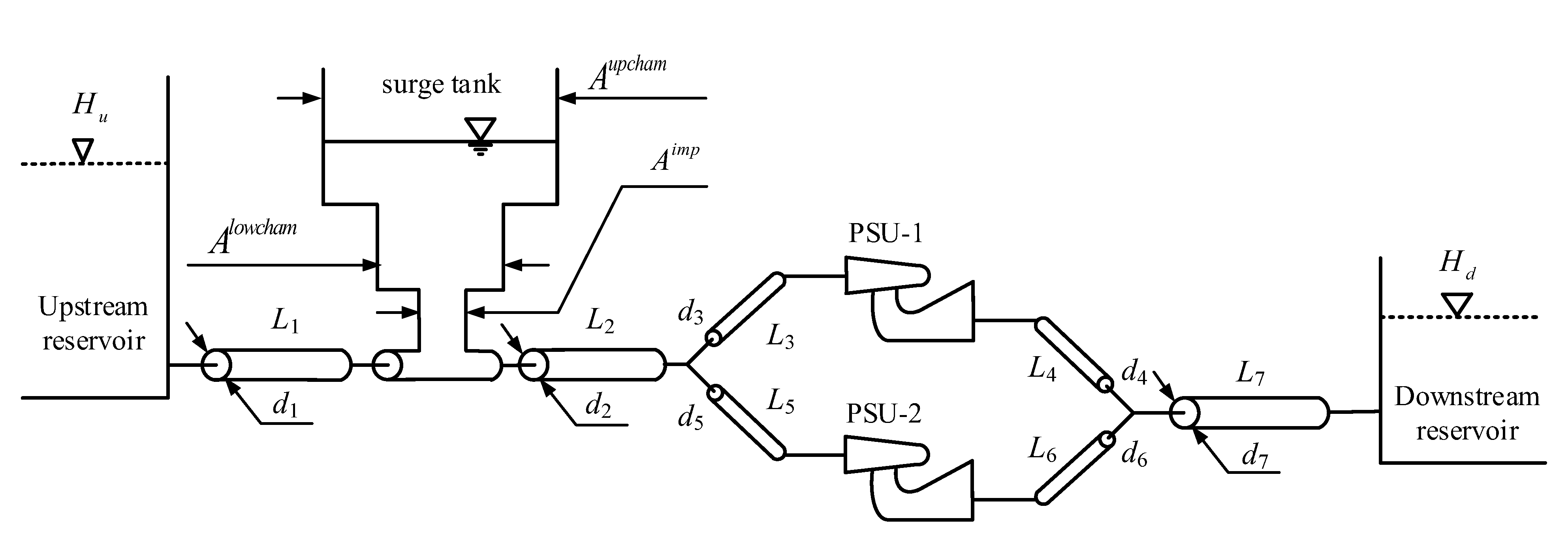
2. Refined Modelling of a Pumped Storage Plant for Back-to-Back Starting

The BTBS mode is also called synchronous starting mode, which uses one PSU as a generator to provide the current with increasing frequency. The other PSU to be started is used as a motor, and the current with variable-frequency output by the former is used to accelerate to the rated speed synchronously. The BTBS is affected by the coupling factors of the hydraulic-mechanical and electrical systems. The basic form of BTBS is shown in Figure 2.

2.1. The Hydraulic-Mechanical Subsystem

(1)
Conduit System
On the basis of hydromechanical theory, the momentum and continuity equations, which describe the unsteady pressure and flow in penstocks, can be formulated as follows [24]:
Q t + g A H x + f 2 d A Q Q = 0
a 2 Q x + g A H t = 0
The details of all variable symbols in the study are presented in the Nomenclature. The MOC method is used to solve the above equations, considering the elasticity of the water hammer in the penstocks [25].
(2)
The Pump turbine Model
As the key equipment of energy conversion, it is crucial to model the pump turbine accurately. At present, the characteristic curves have been widely adopted in nonlinear modelling for pump turbines provided by manufacturers, as shown in Figure 3. The nonlinear model can be described by (3) and (4):
M 11 = f M ( Y , N 11 ) Q 11 = f Q ( Y , N 11 )
M t = M 11 D 3 H t Q t = Q 11 D 2 H t N = N 11 H t / D
As shown in Figure 3, the S-shaped area raises obstacles for the pump turbine modelling, which presents a multivalued characteristic. The Logarithmic-Curve-Projection (LCP) method [13] is proposed to convert the unit speed N11 in the way of logarithmic projection so as to overcome the difficulty. The equation is as follows:
X = n 11 / e q 11 n 11 = N 11 / N 11 r q 11 = Q 11 / Q 11 r
The results obtained by means of the LCP method are shown in Figure 4; the LCP curves reflect the change rule of Q11 and M11 with abscissa X. It immensely reduces the complexity of the calculation procedure problems whether compared with the Suter or improved Suter methods [26].
Thereafter, in a given moment, the unit moment and the unit flow are computed using interpolation in accordance with the LPC curves.
(3)
The Turbine Governor System
The governor of the PSP is comprised of a controller and servomechanism. As the actuator of the governor, the servomechanism uses the output signal of the PID controller to drive the guide vanes. Considering the main nonlinear factors (dead zone, saturation, and output limiting), the whole model of the governor is shown in Figure 5.

2.2. The Electrical Subsystem

(1)
Synchronous Machine
Since it is very difficult to gain an accurate value of the original parameters of the synchronous machine through analysis and calculation, 18 original parameters of a synchronous machine are usually converted into 11 machine parameters composed of steady-state, transient, and sub-transient parameters in engineering, which can be obtained directly through experiments. The mathematical model of a synchronous machine expressed by 11 machine parameters includes voltage balance equations of stator winding (8), excitation equations of stator winding (9), voltage balance equations of rotor winding (10), and a rotor motion Equation (11) [27].
v d = φ ˙ d ω φ ˙ q R a i d v q = φ ˙ q + ω φ ˙ d R a i q
φ d = E q X d i d φ q = E d X q i q
T d 0 E ˙ q = X d X d X d X d E q + X d X d X d X d E q + E f d T d 0 E ˙ q = E q E q X d X d i d T q 0 E ˙ d = X q X q X q X q E d + X q X q X q X q E d T q 0 E ˙ d = E d E d + X q X q i q
δ ˙ = ω 1 ω 0 T j ω ˙ = M t M e
(2)
The Excitation System
A DC exciter is adopted, as shown in Figure 6 [28]. The primary elements of the excitation system block are the lead-lag compensator, main regulator, exciter, and damping block.

2.3. Model Validation with On-Site Measurement

The proposed PSP model is validated by a case study in this subsection. In previous studies, in many cases the electrical subsystem model has been validated by measurement [29]. Therefore, the goal of this paper is to use the model to prove the hydraulic-mechanical subsystem.
The research data in this section are from a large PSP in Hubei Province of China, and the topology of its regulation system is shown in Figure 7. The parameters of the pump turbine and the generator and motor of the PSU are shown in Table A1, and the characteristic curves of the pump turbine are shown in Figure 3. The pipeline parameters of the diversion system that can be used for modelling after processing are shown in Table A2. The dimensional parameters of the surge chamber are shown in Table A3. In addition, the basic parameters of each module of the regulation system are shown in Table A4.
In this case study, PSU-2 is offline when PSU-1 begins a single-unit load rejection. The water level of the upper reservoir is 306.98 m, and the downstream reservoir is 96.11 m, so the gross head is 210 m. When the PSU-1 operates normally with 300 MW load, the load is suddenly rejected. The guide vane is normally closed in 30 s. The variation waveform of various parameters in the simulation test is shown in Figure 8. Through analysis of the graph, the characteristic values of each parameter change are extracted and compared with the results of field measurements. Table 1 shows the comparison results.
As revealed in Figure 8 and Table 1, the calculation results of the full load rejection transition process achieve consensus results with the on-site measurements, which effectively verifies the accuracy of the PSP mathematical model constructed in this paper.

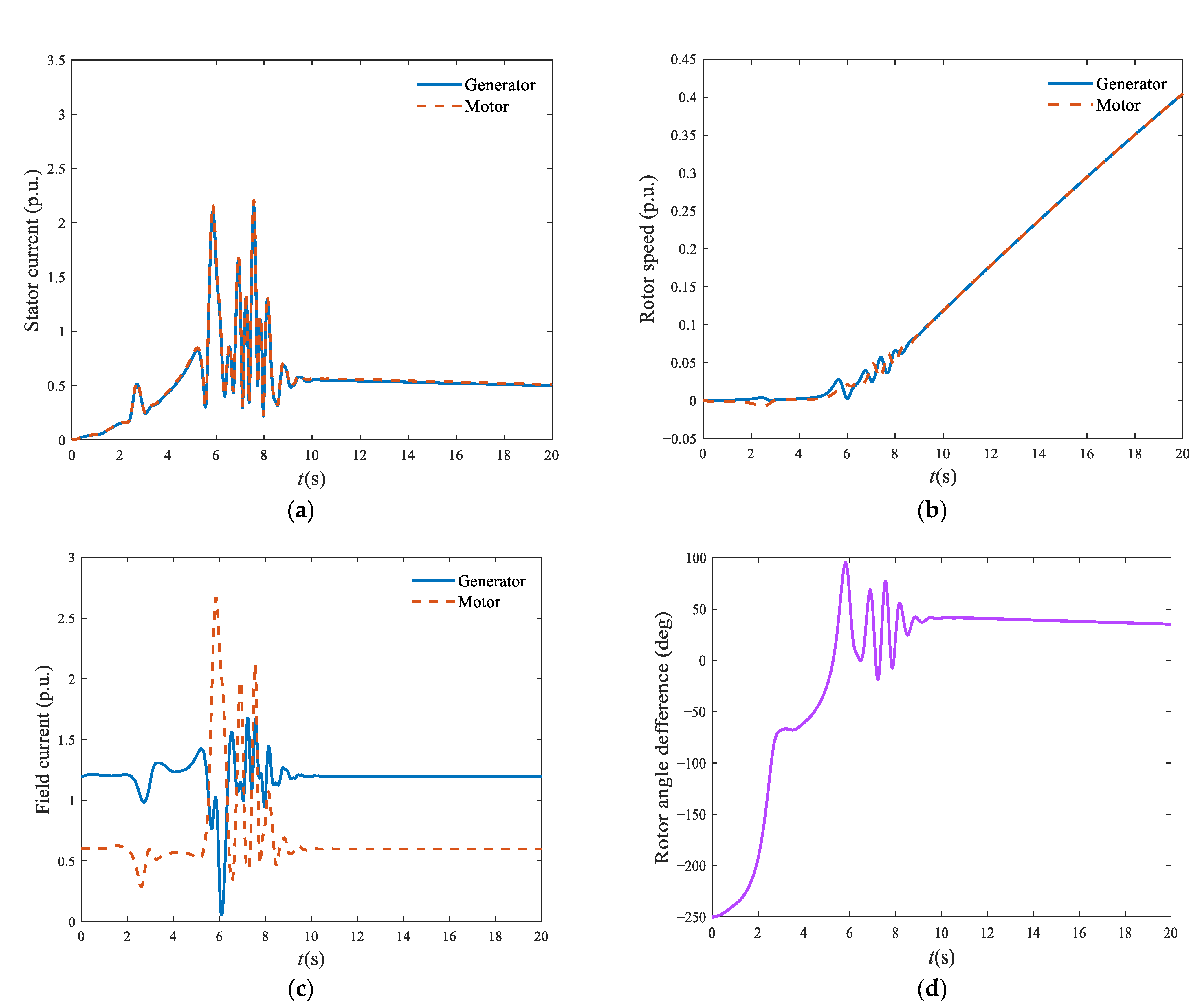
3. Analysis of Factors Affecting Back-to-Back Starting

3.1. Excitation Current

The excitation system of the two units adopts separate excitation sources (grid-side power supply or auxiliary power supply), and the closed-loop control modes of the constant excitation current (CEC) are adopted for the two units. After the speeds of the two units are synchronously accelerated to 90% of the rated value, the excitation control modes are changed to the closed-loop working modes of the constant terminal voltage. Figure 9 is an example of successful BTBS (given excitation current i g * = 1.2 , i m * = 0.6 ), while Figure 10 is an example of a failed start due to improper matching of excitation current (given that excitation current i g * = 0.8 , i m * = 0.5 ).
To explore the impact of given excitation current ( i g * , i m * ) on the BTBS process, BTBS under different excitation currents ( i g * , i m * ) are simulated, as may be observed in Figure 11. The range of i f d * is [0, 2], the default values are kept for other parameters of the PSP.
In Figure 11, The blue circle within the green area means that the BTBS is successful when the excitation current is ( i m * , i g * ). It shows that the BTBS results are altered by the given excitation current. The excitation current of the generator and motor must maintain an appropriate proportion to ensure successful BTBS. In particular, the proportion is affected by the characteristics of the units, and the requirements of the excitation current for the units are also different.

3.2. Control Way of the Excitation System

There are usually four control modes of an excitation system: constant terminal voltage regulation, constant excitation current regulation, constant reactive power regulation, and constant power factor regulation [30]. However, in the BTBS process of a large PSU, the excitation mode is usually constant excitation current regulation or constant terminal voltage regulation.
One innovation of this paper is the discovery that the closed-loop working mode of constant excitation voltage (CEV) (Note: not constant terminal voltage) can also realize BTBS. Two control modes are simulated and compared. For the convenience of comparison, only the oscillation stages before the two machines run into synchronous acceleration are presented. The simulation results of BTBS with CEC ( i g * = 1.4 , i m * = 1.2 ) are shown in Figure 12. Figure 13 shows the simulation results of BTBS with CEV ( V g * = 1.4 , V m * = 1.2 ).
By studying Figure 12 and Figure 13, it is revealed that under the same initial conditions, the oscillation in the starting process of CEC is much larger than in that of CEV. The above physical process shows that there must be an oscillation process when the two machines enter the oscillation stage before synchronous acceleration. The rotor circuit passively plays a specific damping role in this oscillation process, and the excitation current will oscillate accordingly. If the CEC closed-loop mode is adopted, the excitation current of the two machines will be forced to remain constant, which will weaken the damping effect of the rotor circuit. When the closed-loop mode of CEV is adopted, the excitation current of the two machines is allowed to oscillate passively to a certain extent, which is equivalent to increasing the damping of the rotor circuit. In this way, the excitation circuit should adopt the closed-loop mode of CEV.

3.3. Initial Difference between Rotor Positions
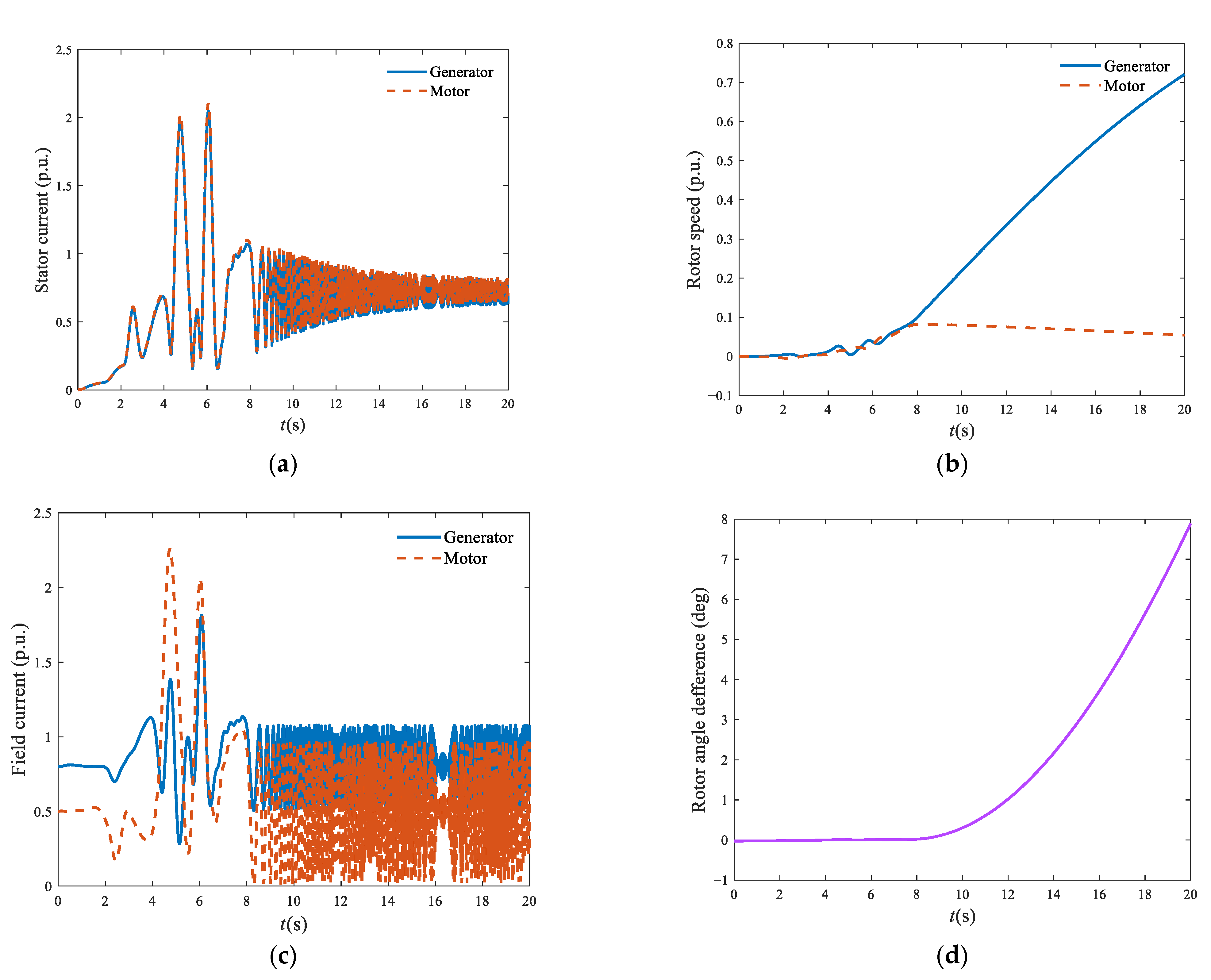
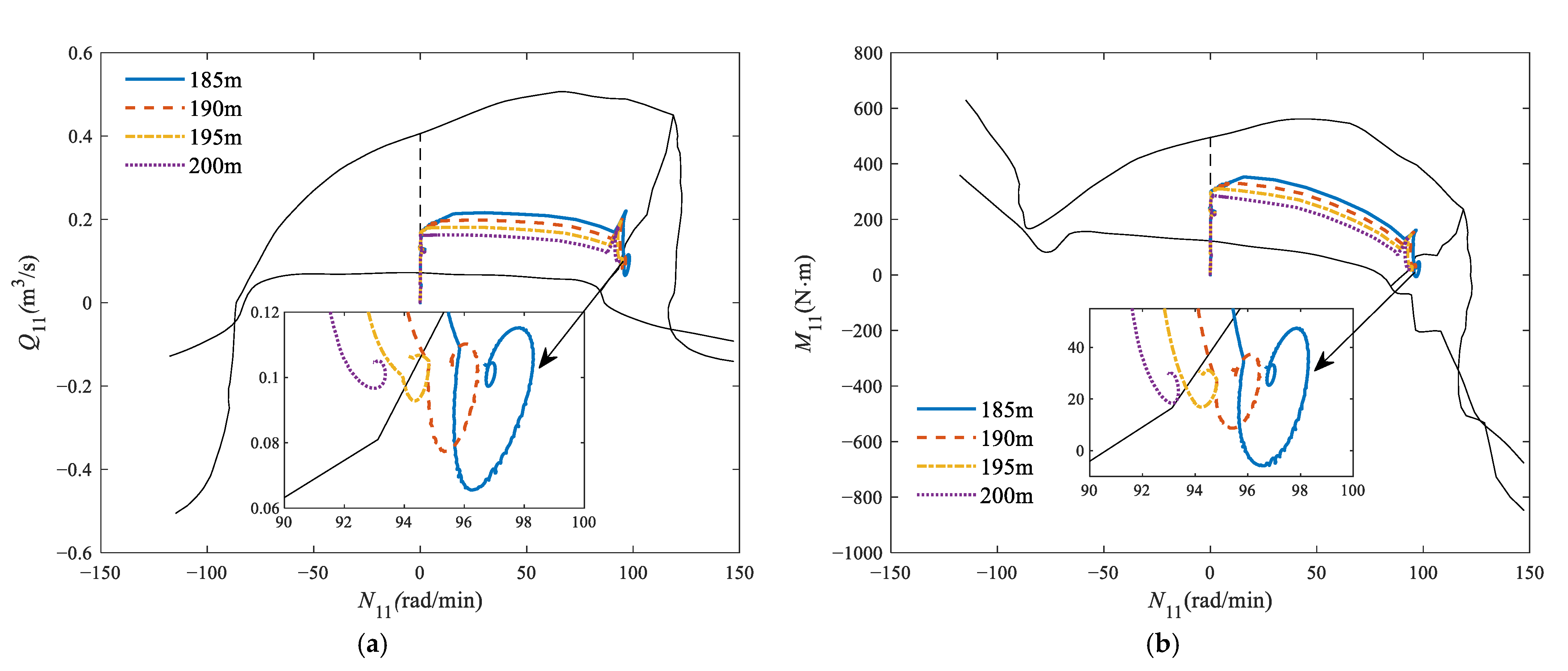
Due to the randomness of the initial difference between rotor angles of two units, there must be an adjustment from the initial angle difference to the target angle difference, which begins after the water pump is started. Table 2 shows the BTBS results of the two machines under different initial angles. The variation of rotor angle difference under different initial conditions is shown in Figure 14.
By observing the simulation results, it can be observed that different initial rotor angles have a certain impact on the startup time of the unit, but have little impact on the target angle difference when the rotor angle difference is stable. With the change of initial rotor angle difference between units, the oscillation in the startup synchronization will change to varying degrees, but it will not affect the successful startup of the unit. Therefore, the influence of the initial difference between rotor positions on BTBS may be ignored.

3.4. Water Head

As an important working condition parameter, the working head is also one of the pivotal influencing factors of the hydraulic machinery transition process, which can be roughly estimated by the water level difference between the upper reservoir and lower reservoir. Here, the changes in water levels above and downstream represent the changes in the working head of the pump turbine, and explore the influence of the working head on BTBS. Therefore, based on the actual unit data of a large PSP in China and the refined model of the PSU, the BTBS process under different working heads is simulated by numerical simulation in this section. The actual data of the unit is as follows: the maximum working head is 217 m, the rated working head is 195 m, and the minimum working head is 178.1 m. Figure 15 shows the dynamic process trajectory curve of unit flow and unit torque of the tractor under the working head of 200 m, 195 m, 190 m, and 185 m during the BTBS process. For the convenience of comparison, the critical multivalue points of each opening line on the flow characteristic curve and torque characteristic curve are connected to obtain the critical flow line and torque critical line dividing the S-shaped area, as shown in Figure 16. The critical boundary divides the closed area consisting of 0 unit velocity line, 6.9% opening line and 100% opening line into two parts. On the right is the S-shaped area and on the left is the area that can work steadily.
As observed in Figure 15, with the decrease of the working head, the opening of the no-load guide vane of the corresponding back-to-back starting tractor gradually increases. At this time, the unit can easily fall into the S-shaped area at the working point of rated speed. The strong nonlinearity of the pumped storage system in the S-shaped area and the instability of the control system act upon each other, especially when the PSU operates at 185 m head; the flow and torque in the S-shaped characteristic area fall into chaotic operation. This dynamic characteristic will lead the unit speed to swing to and fro, leading to a repeated adjustment of the guide vane opening. If there is no appropriate control strategy, the BTBS process of the unit under a low water head will fail. In summary, under the back-to-back starting condition, the lower the working head of the pump turbine, the more unfavorable it is to the hydraulic mechanical transition process of the unit.

3.5. Control Scheme of the Governor

The BTBS process consists of both open-loop and closed-loop control. The strategy of slowly opening of the guide vane to a certain set point (related to the current water head) is adopted before the rotor speed of the driving machine reaches a certain value ωs. After accelerating to 0.9, the PID controller is put into operation in closed-loop regulation according to the rated speed, as shown in Figure 17. The rotational speed transition curves of BTBS are plotted at different points of starting time Ts in Figure 18. Generally, the faster the guide vanes are opened, the faster the speeds of the units rise, but this is not absolute. As shown in Figure 18, when the starting time Ts =15 s, the rising speed of the driven machine is faster than the scheme with starting time Ts =10 s.

4. Optimization of BTBS Strategy Based on Multi-Objective Control

It is evident from Section 3 that the excitation current, control way of the excitation system, and control scheme of the governor have a marked impact on the BTBS process. It may even be unsuccessful under the low water head combination of worse control parameters, which is defined as the worst operating condition of BTBS. Therefore, this paper selects the working condition under a low water head as the research object.
The MOPSO algorithm [31,32] is introduced to complete the multi-objective optimization of the BTBS strategy. MOPSO is extensively used in many industries and has outstanding performers in the control optimization of PSU due to its superiority of easy implementation, high precision, and fast convergence [33,34].

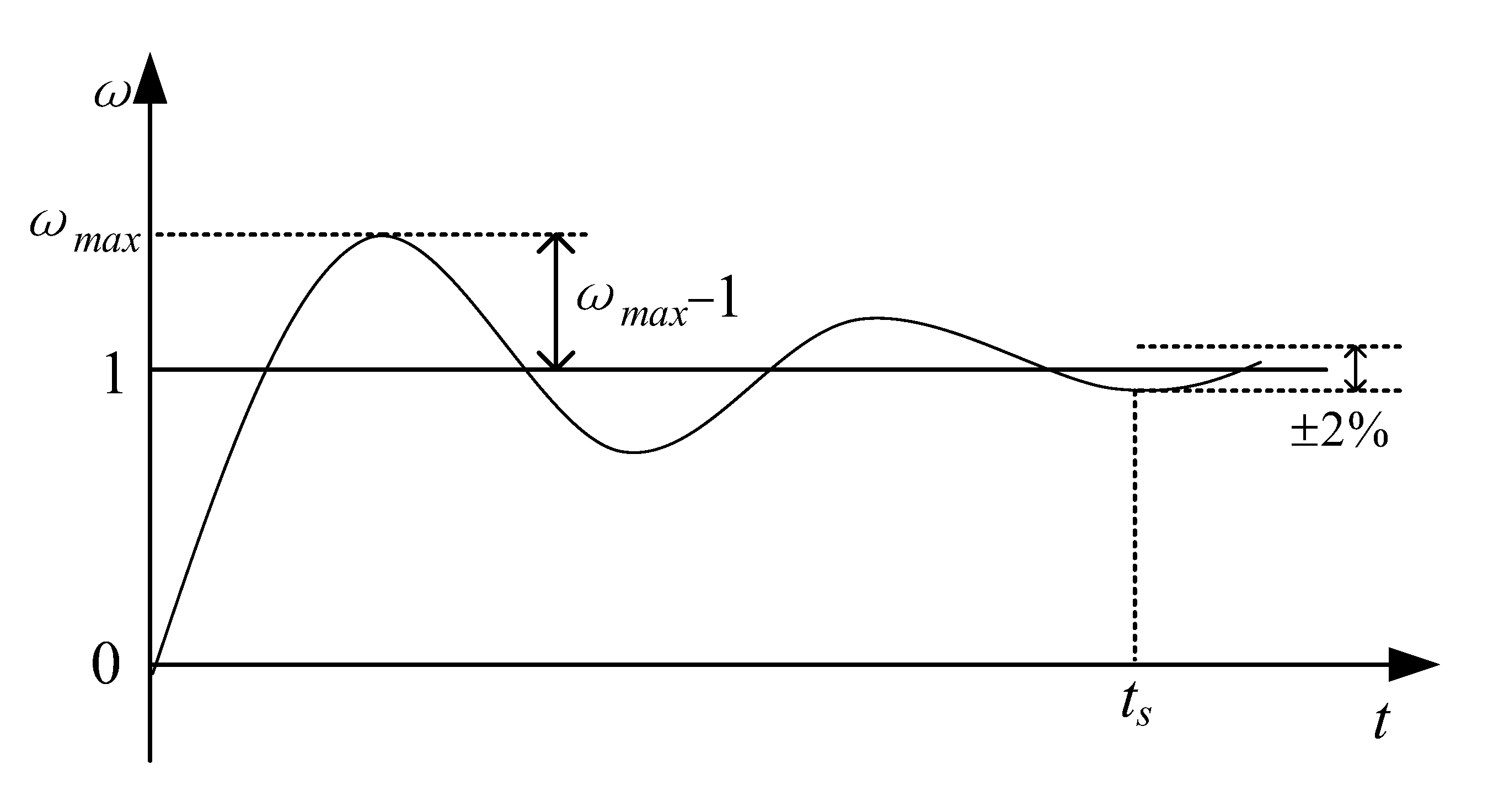
4.1. Objective Function

In the BTBS process, the overshoot of rotational speed and the speed stable time can be chosen to respectively represent the stationarity and the rapidity on which we focus. Thus, the overshoot and stable time of rotational speed are included as the evaluation indexes to optimize the BTBS strategy on the basis of multi-objective control. While both evaluation indexes are substitutes, the velocity is more critical, so the speed overshoot of PSU-1 and speed rise time of PSU-2 are chosen as two optimization indexes.
The two objectives are defined as follows:
min F 1 = ω 1 max 1 min F 2 = t s 2
where ω 1 max is the relative value of the peak speed of driving machine PSU-1, and t s 2 is the speed stable time of driven machine PSU-2. The description of the objective function is shown in Figure 19.

4.2. Decision Variables

The decision variable is the parameter of the BTBS strategy. For convenience of analysis, the speed regulation strategy adopts “one-stage guide vane direct opening + PID control”, as shown in Figure 17. This paper studies two excitation strategies: constant excitation current (CEC) and constant excitation voltage (CEV). Their decision variables are summarized as follows:
  • Scheme 1: The traditional CEC mode with one-stage DGVC+PID control. In one-stage DGVC, the guide vane of the driving machine is first opened at the rate kc, and remains unchanged when the guide vane opening reaches yc. When the speed reaches 90% of the rated speed, the PID controller will be put into operation. The excitation system of the two units shall first operate with the given excitation current, and switch to the constant terminal voltage mode when the speed reaches 90% of the rated speed. kc generally takes the maximum rate, which is a known parameter. Therefore, the given excitation current i g * , i m * , and given opening yc are selected as the decision variables in the open-loop stage. Parameters of PID controller, Kp, Ki, and Kd, are adopted as the decision variables in the closed-loop stage.
    X 1 = i g * , i m * , y c , K p , K i , K d
  • Scheme 2: The proposed CEV mode with one-stage DGVC+PID control. Similarly, the given excitation voltage V g * , V m * , given opening yc, and the three parameters of PID controller, Kp, Ki, and Kd, are chosen as the decision variables.
    X 2 = V g * , V m * , y c , K p , K i , K d

4.3. Constraint Conditions

There are three types of constraints extracted from engineering limitations according to our experiments in this study.
(1)
Operation Time Constraint
0 < t s 2 < t max
where t s 2 is the stability time of PSU-2. t max is the maximum operation time.
(2)
The Boundary of Decision Variables
X i L , U
where X i is the decision variables of i - th scheme; L and U indicate the lower limits and the upper limits of the boundary.
(3)
Rotor Speed Difference Between Two Machines
According to the requirements of the BTBS, the rotational speed difference between the two units shall not exceed a certain limit value; otherwise, it is considered a startup failure:
ω 1 ω 2 ω max d
where ω 1 is the rotor speed of the driving machine and ω 2 is the rotor speed of the driven machine. ω max d is the maximum allowable rotor speed difference between the two units.

4.4. Optimization Procedures

Based on the nonlinear simulation platform of the PSP system, this study puts forward two multi-objective optimization schemes of BTBS strategy, which are multi-objective constant excitation current (MOCEC) and multi-objective constant excitation voltage (MOCEV). In this subsection, the MOPSO algorithm is introduced to optimize the proposed optimization scheme under the low head condition of BTBS, because once the optimized control schemes can be applied to poor conditions, it is able to adapt to those under normal circumstances. Figure 20 shows the flowchart of the optimization for BTBS with main optimized procedures.

5. Case Study and Analysis

A real PSP in China is taken as the experimental object for the simulation analysis so as to certify the efficacy of the proposed scheme. The layout of the power station is shown in Figure 7. Both units participate in operation; that is, one pipe and two units operate under BTBS conditions. Among them, 1# machine operates as a tractor under the power generation condition of water turbine, and 2# unit operates as a driven machine under the pumping condition of the motor.

5.1. Model Parameters Setting

As shown in Figure 7, the capacities of the two units are the same. The basic parameters of the water diversion system, pump turbine, synchronous machine, governor, and excitation system are the same as those in Section 2.3, as shown in Table A1, Table A2, Table A3 and Table A4. All experiments in this section are carried out under the identical water head; that is, the water level of the upstream reservoir is 291.45 m, and that of the downstream reservoir is 106.11 m. The parameters of the multi-objective optimization algorithm are set as follows: the number of iterations is 200, the population size is 50, the initial value of the inertia weight is 0.5, the size of the external archive is 25, the inertia weight damping is 0.99, and the acceleration constants c 1 and c 2 are both 1.6. According to the analysis of experimental experience and results, the value ranges of decision variables X1 and X2 are obtained, as shown in Table 3.
The multi-objective optimization results named Pareto Set need further ordering to acquire the optimal solution that satisfies the needs of the decision-maker. Therefore, in this section, the multi-objective decision-making method based on relative target proximity is also used to sort the Pareto optimal solution set of MOCEC and MOCEV [35], and the weight information consisting of subjective weight α , objective weight β , and comprehensive weight γ required by the decision-making method are given in Table 4.

5.2. Introduction to Comparative Experiments

In order to demonstrate the superiority of the schemes mentioned above, single-objective optimization schemes based on the PSO algorithm are designed as comparative experiments, which are abbreviated as single objective constant excitation current (SOCEC) and single objective constant excitation voltage (SOCEV). The integrated time and absolute error (ITAE) index can be obtained for each unit, as shown in Equations (15) and (16):
F I T A E 1 = k = 1 N s t ( k ) | 1 ω 1 ( k ) |
F I T A E 2 = k = 1 N s t ( k ) | 1 ω 2 ( k ) |
where subscript 1 represents the variable of 1# unit, subscript 2 represents the variable of 2# unit. In order to consider the dynamic process performance indexes of the two units at the same time, the ITAE indexes of the two units are integrated with certain weights w 1 and w 2 as an objective function, as shown in Equation (17):
F I T A E = w 1 F I T A E 1 + w 2 F I T A E 2
where F I T A E is the objective function of single objective scheme, and w 1 and w 2 are the weight of ITAE index of 1# unit and 2# unit respectively.

5.3. Effectiveness Analysis

For the MOCEC and MOCEV, the optimization result is a set of Pareto optimal solution sets. The particles in the Pareto optimal solution set are non-dominated solutions to each other. The particles in the Pareto optimal solution set are listed in Table A5 and Table A6. To make the optimal solution satisfy the needs of the decision-maker, the decision-making method based on relative target proximity is used to sort the particles in the Pareto optimal solution set. The weight value of the decision-making method is shown in Table 4, so the particle ranking is selected as the optimal solution for the multi-objective optimization scheme. Table 5 shows the optimal solutions of the four schemes.
The optimal decision variables of the four schemes correspond to the four optimal BTBS strategies. The transition process curves of 1# and 2# units under BTBS conditions can be obtained by inputting the four optimal startup strategies into the nonlinear simulation platform of the PSP, as shown in Figure 21. Due to the short adjustment time of field current and rotor angle difference, these two parameters only show the transition process of the first 10 s. The performance indexes of rotor speed are shown in Table 6; Δωmax represents the speed overshoot, tr represents the speed rise time, and ts represents the stability time.
In Figure 21a, it can be found that the speed overshoot of single-objective schemes is large, while the speed overshoot of multi-objective schemes is small; the speed fluctuation of multi-objective schemes is also small and the curves are more stable. Figure 21b shows the PSU-2′s speed transition processes of the four schemes. It can be observed that the speed curves of single-objective schemes fluctuate more, and the speed curves of the multi-objective schemes are more stable. Figure 21c–h shows the transition curves of other physical quantities. In Figure 21c–d, the field current regulation processes of the four schemes have a certain fluctuation, but the current transition process curve of the MOCEV scheme can reach the steady state fastest and the fluctuation is the smallest. In Figure 21e, the GVO adjustment process of the MOCEV scheme is faster and the oscillation times are the shortest. As seen in Figure 21f, the peak value of rotor angle difference of the four schemes is essentially the same, but the rotor angle fluctuation range of the MOCEV scheme is the smallest. As observed in Figure 21g, the terminal voltage rise processes of the four schemes are slightly different. The terminal voltage rise of the single-objective optimization methods is faster than those of the multi-objective optimization methods, and the impulse generated during voltage control switching of the CEC control scheme is smaller than that of the CEV control scheme. By observing Figure 21h, it can be concluded that during the BTBS under low water head conditions, the multi-objective optimization method can help the PSU avoid going deep into the S-shape zone, so as to avoid the repeated oscillation of active power and falling into chaos. Therefore, from the analysis of other working indexes of the two units, the multi-objective optimization schemes are better than the single-objective optimization schemes.
For the single-objective schemes, the objective function is the weighted sum of the ITAE indexes of two units. It can be obtained from Table 6 that the speed overshoot of 1# unit is 4.98% and the speed rise time of 2# unit is 26.82 s for SOCEV, which is less than the value of SOCEC, but the speed stable time of 1# and 2# unit of SOCEC are slightly less than the value of SOCEV. For the multi-objective schemes, the objective function is speed overshoot of PSU-1 and speed stable time of PSU-2. The speed overshoot of 1# unit is 0.00088% and the speed stable time of 2# unit is 58.98 s for MOCEV, which is less than the value of MOCEC. Furthermore, comparing different schemes, the speed overshoot of multi-objective optimization schemes is much smaller than those of single-objective optimization schemes, and the speed stable time of multi-objective optimization schemes is also smaller. However, the speed rise time of multi-objective optimization schemes is greater than those of single-objective optimization schemes. In addition, among the four schemes, the speed overshoot of PSU-1 and speed stable time of PSU-2 for MOCEV are the smallest, so it is considered that the optimization effect of the MOCEV scheme is better.
To further reflect the advantages of the multi-objective scheme MOCEV, Figure 22 shows the Pareto fronts of MOCEC and MOCEV schemes.
The Pareto front are even-distributed shown in Figure 22, and the first 25 particles of the MOCEV scheme are non-dominated solutions. If one selects three particles from the far left, middle, and far right for specific analysis, one could simulate their speed transition process curve, as shown in Figure 23. In Figure 23, the speed overshoot of 1# unit of three particles increases in turn, while the speed stable time of 2# unit decreases in turn. Additionally, these three typical particles can help the unit avoid going deep into the S-shaped zone, which ensures the safety and stability of the BTBS process of the PSU under low head conditions. These three particles represent three kinds of particles. Decision-makers may choose one of them as the optimal solution for power plant operation according to actual needs. There are also 25 particles in front of the MOCEC scheme, and most of them are dominated by the particles at the front of the MOCEV. This phenomenon also shows that the MOCEV scheme is better than the MOCEC.

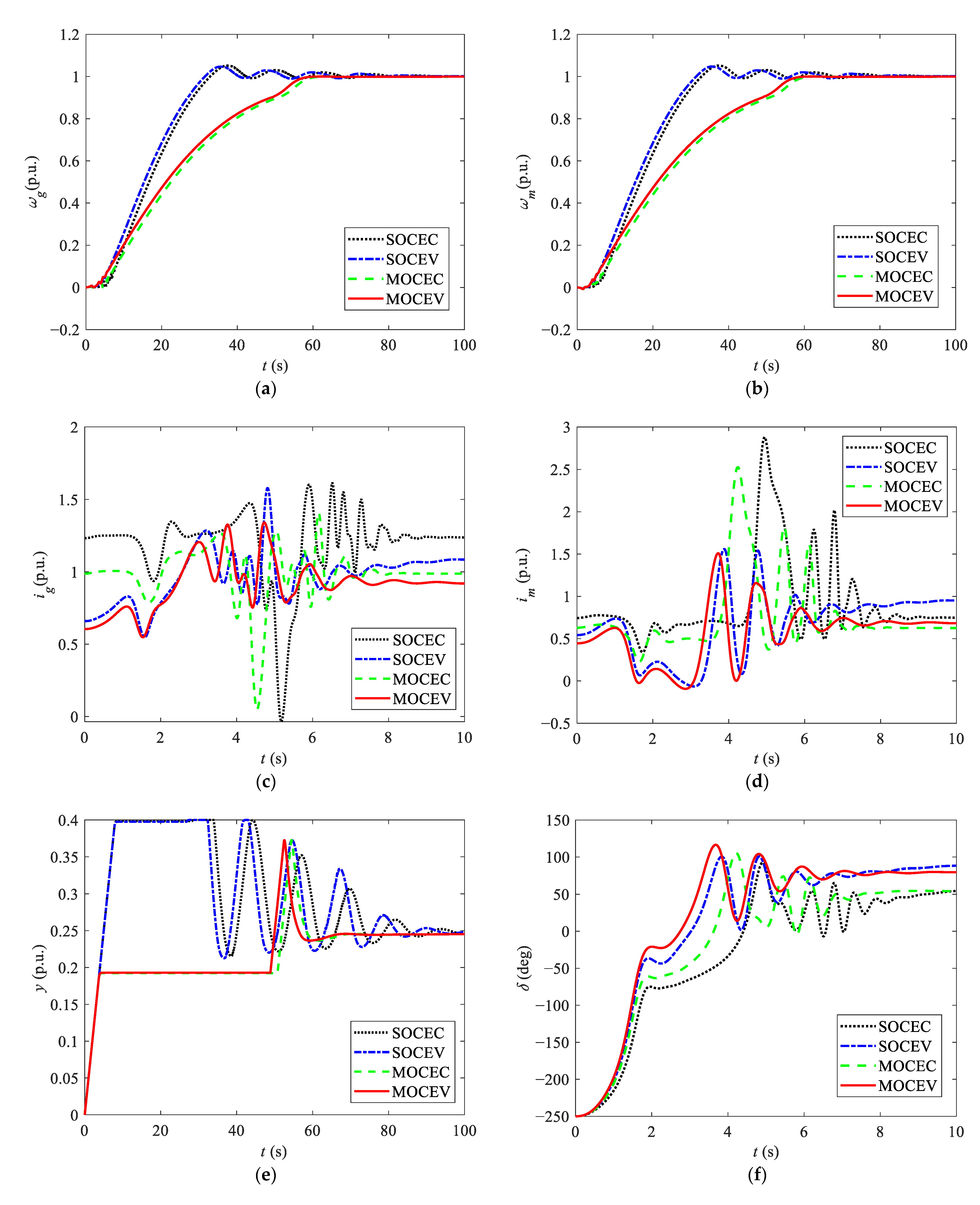
5.4. Validation of the Proposed Optimization Strategy

This section verifies the effectiveness of the multi-objective optimization method MOCEV for BTBS conditions proposed in this paper under other conditions, and selects different upstream and downstream water levels to form the verification conditions; the corresponding data are listed in Table 7. The parameters of the optimization results in Section 5.4 are respectively substituted into the refined mathematical model of the regulation system of the PSU for the transition process simulation, and the key indicators of the transition process are obtained, as shown in Figure 24.
Figure 24a–c shows that, when the multi-objective optimization result is used as the control parameter for BTBS, with the water head increases, the velocity overshoot increases, the velocity stable time decreases first and then increases, and the speed rising time decreases. This is because the no-load GVO under a low water head is larger. When used for open-loop control under other water heads, the speed rise will be faster and the overshoot will be increased. However, in order to ensure that the unit does not fall into the S-shaped area, the integral parameter value under the low head is small, which will lead to a longer time for the speed to reach the steady state under other conditions. Therefore, with the increase of water head, the integral parameters can be appropriately increased to improve the regulation quality under other working conditions. In addition, by observing Figure 24d, it can be concluded that the control parameters optimized under a low water head can prevent the BTBS process of the unit from falling into the S-shaped zone within the full working condition.

6. Conclusions

A refined nonlinear model for BTBS of PSP is developed in this paper, the impacts from the electrical and hydraulic-mechanical subsystem on the operation of PSP during BTBS are investigated subsequently, and a novel MOCEV control strategy is proposed accordingly. The following conclusions are drawn from the simulation results.
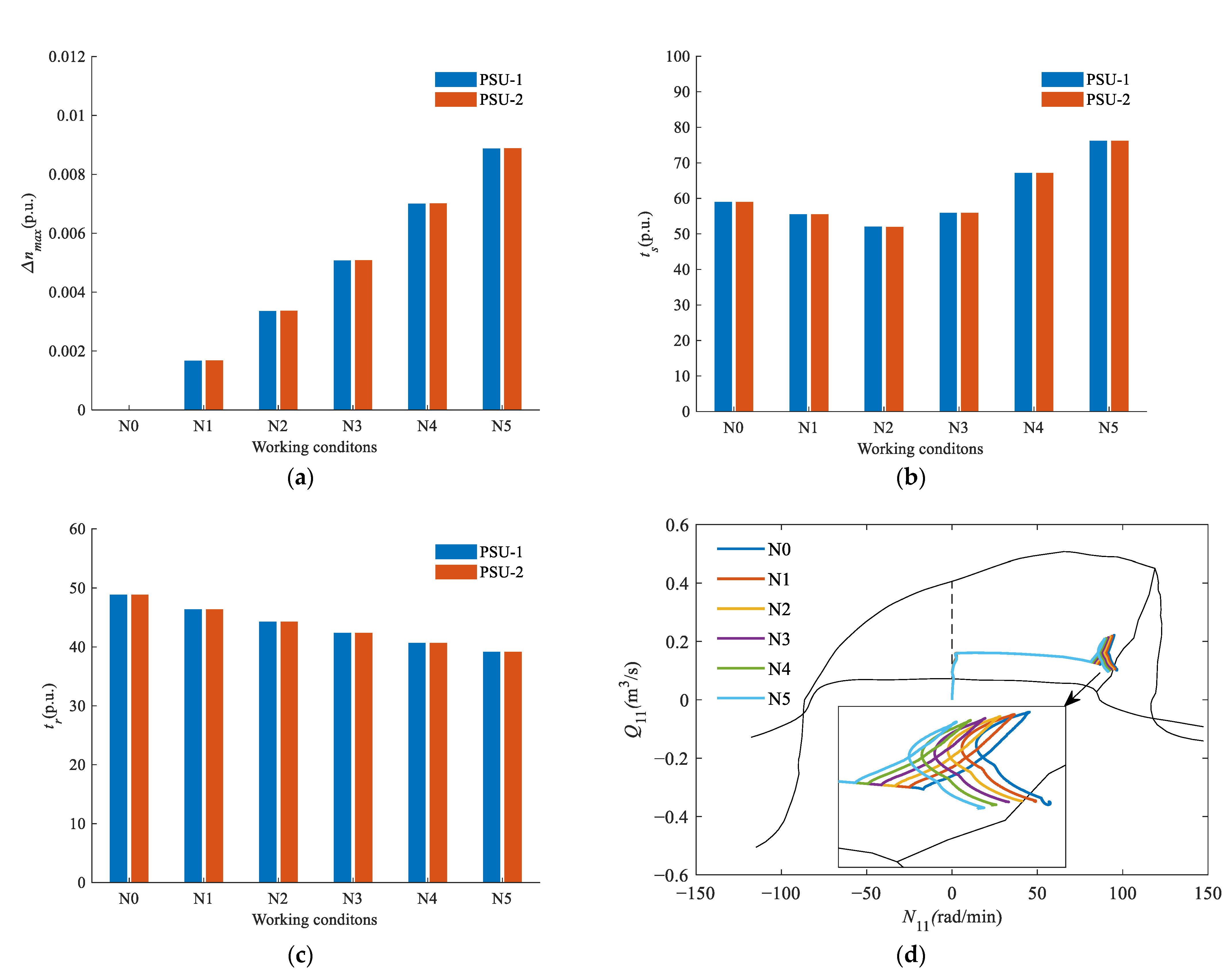
  • The given value and control way of excitation current, the control scheme of the governor, and the water head have great influence on the transient process of BTBS. The control scheme of excitation current and guide vane should be selected as the decision variables in the BTBS optimization; the worst BTBS condition can be identified by the lowest water head.
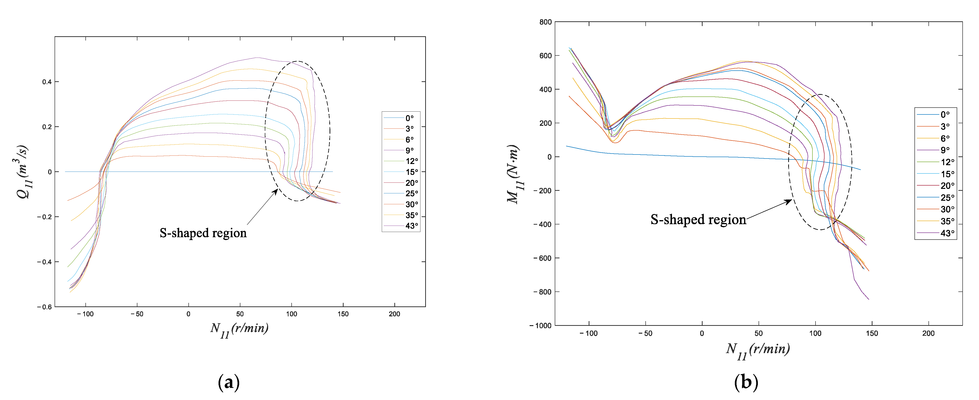
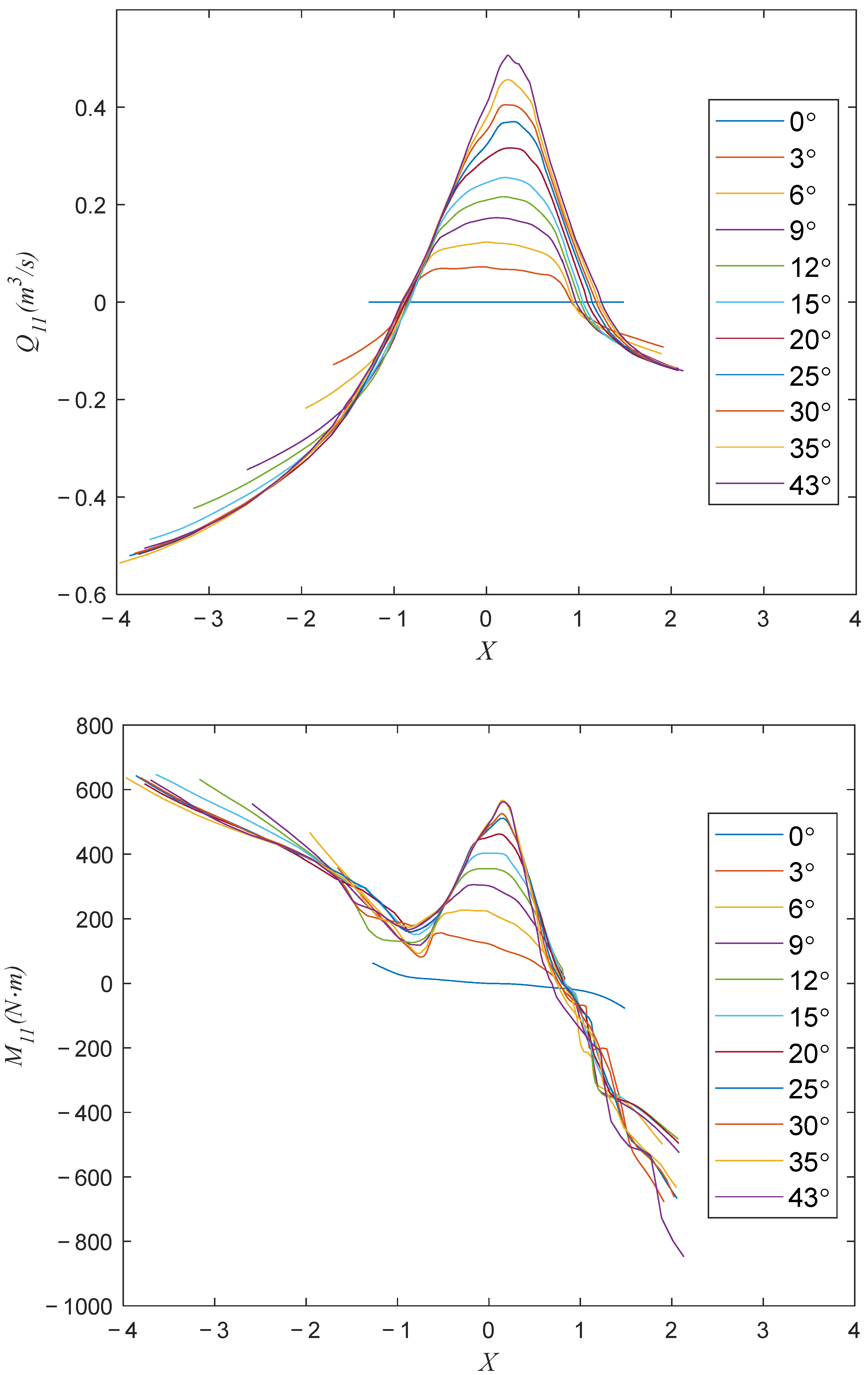
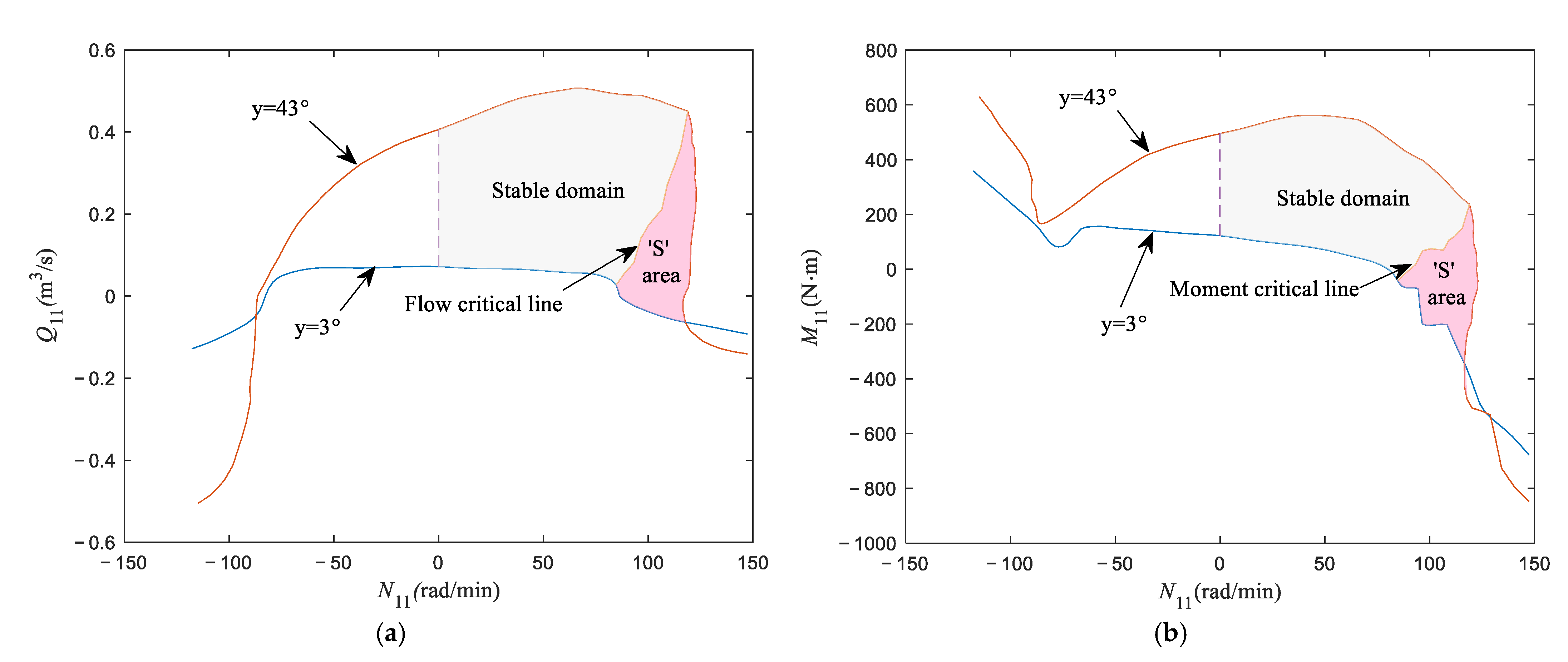
  • The overshoot and stable time of the speed are contradictory. The traditional single-objective optimization scheme merely considers the single objective, which can very easily cause the unit to fall into the S-shaped area, resulting in severe fluctuations in speed and power.
  • Compared with the single-objective, the optimization strategy proposed can considerably improve the speed overshoot and the speed stable time by at least 68.27% and by 3.22% under the worst working condition. The optimization results show that the multi-objective scheme is a better choice than the single-objective scheme.
  • Compared with the MOCEC scheme, when the MOCEV scheme is adopted, the overshoot, rise time, and stable time are improved by 68.35%, 3.7%, and 3.2% in PSU-1, and 45.4%, 3.7%, and 3.2% in PSU-2. Thus, the MOCEV scheme is superior.
  • The proposed MOCEV optimal control scheme can effectively keep away from the S-shaped area and is verified by a real PSU.

Author Contributions

Conceptualization, methodology, software, data curation, writing, original draft preparation, C.F.; writing, editing, corresponding, G.L.; reviewing and editing, supervision, Y.Z.; supervision, D.Z.; visualization, investigation, Z.M. All authors have read and agreed to the published version of the manuscript.

Funding

The Fundamental Research Funds for the Central Universities (B220202005) and the National Natural Science Foundation of China (No. 51979086).

Institutional Review Board Statement

Approval for the study was not required in accordance with local/national legislation.

Informed Consent Statement

Not applicable.

Data Availability Statement

Not applicable.

Conflicts of Interest

The authors declare that they have no known competing financial interest or personal relationships that could have appeared to influence the work reported in this paper.

Nomenclature

Abbreviations
PSPpumped storage plant
BTBSback-to-back starting
PSUpump storage unit
CEVconstant excitation voltage
CECconstant excitation current
LCPlogarithmic curve projection
MOCmethod of characteristics
GVOgate valve opening
MOCECmulti-objective CEC
MOCEVmulti-objective CEV
SOCECsingle-objective CEC
SOCEVsingle-objective CEV
ITAEintegrated time and absolute error
puper-unit value
Symbols
Parameters
Across sectional area of pipeline (m2)
awave velocity (m/s)
bppermanent difference coefficient (pu)
Dthe diameter of the turbine runner (m)
dpipeline diameter (m)
ffriction coefficient (pu)
gacceleration of gravity (m/s2)
Kddifferential gain (pu)
Keself-excitation coefficient of exciter (pu)
Kfdamping coefficient (pu)
k0forward amplification factor (pu)
Kiintegral gain (pu)
Kpproportional gain (pu)
Raresistance of stator winding (pu)
Seexciter saturation factor (pu)
Taamplifier time constant (s)
Tblead lag time constant (s)
Tclead lag time constant (s)
xdistance calculated from upstream (m)
Tddifferential time constant (s)
Teexciter time constant (s)
Tfdamping time constant (s)
Tjmechanical time constant (s)
Tymain servomotor response time (s)
Ty1assistant servomotor response time (s)
T d 0 , T d 0 transient and sub-transient time constants of open-circuit d-axis (s)
T q 0 , T q 0 transient and sub-transient time constants of open-circuit q-axis (s)
X q , X q , X q synchronous, transient and sub-transient reactance of q-axis (pu)
Variables
E d , E d the transient and sub-transient internal EMF of d-axis (pu)
Efdexcitation EMF (pu)
E q , E q the transient and sub-transient internal EMF of q-axis (pu)
Hpiezometric head (m)
Htthe working head of pump turbine (m)
i d , i q the current of d- and q-axis (pu)
ifdexcitation current (pu)
i g * , i m * excitation current setting value of generator and motor (pu)
Kaamplifier coefficient (pu)
Meelectromagnetic torque (pu)
Mtthe moment of pump turbine (pu)
M11unit torque (N/m3)
Nthe rotational speed of the turbine (r/min)
N11unit speed (m1/2/s)
N11rrated unit speed (m1/2/s)
Qthe water flow rate (m3/s)
Qtthe flow of pump turbine (m3/s)
Q11unit flow (m1/2/s)
Q11rrated unit flow (m1/2/s)
ucontroller output signal (pu)
V g * , V m * excitation voltage setting value of generator and motor (pu)
v d , v q d- and q-axis component of the voltage (pu)
Yguide vane opening (deg)
ymain servomotor output signal (pu)
ω, ω*relative and given value angular shaft velocity (m)
φ d , φ q the internal EMF of d- and q-axis (pu)
δ rotor angle (rad)

Appendix A

Table A1. PSP design parameters.
ParametersValuesParametersValues
Rated speed (r/min)250Rated capacity (MVA)334
Rated water-head (m)195Rated voltage (kV)15.75
Rated water flow (m3/s)176.1Rated current (A)12,244
Power rating (MW)306Rated frequency (Hz)50
Turbine runner diameter (m)5.26Power factor0.90
100% guide-vane opening (°)43.01Moment of inertia (ton/m2)19,300
Table A2. Basic parameters of equivalent pipeline of diversion system.
NumberLength (m)Diameter (m)Wave Velocity (m/s)Roughness
L11113.949.2111000.014
L2206.718.9711200.014
L3250.774.7712040.011
L4173.526.9011610.010
L5260.304.8012040.011
L6173.526.8911600.012
L7295.2710.8210500.014
Table A3. Basic parameters of surge chamber.
Sectional Area of the Impedance Hole (m2)Inflow Loss CoefficientOutflow Loss CoefficientSectional Area (m2)Altitude (m)
19.630.00092170.000676719.63231.70~268.30
380.13268.30~310.00
530.93310.00~320.00
Table A4. Basic parameters of each module of the regulation system model of pumped storage unit.
Excitation SystemSynchronous Machine
Ta0.001Ra0.00125X’’d0.2
Tb0Xd1.015X’’q0.195
Tc0Xq0.627Td012.6
Te0Xd0.253T’’d00.189
Tf0.1Tj10.8T’’q00.519
Ka300Speed Regulation System
Ke1bp0.01k01
Kf0.001Ty10.02Ty0.2
Table A5. The detailed parameters corresponding to the Pareto front solutions of constant excitation current.
Solutions F 1 F 2 ( s ) i g * i m * y c KpKiKd
1 0.0000 61.1400 0.9805 0.6135 0.1923 3.4725 0.1000 5.1410
20.0000 60.9600 0.9881 0.6272 0.1924 3.5060 0.1000 4.9311
30.0001 60.8600 1.0098 0.6266 0.1932 3.4515 0.1000 5.0734
40.0002 60.3600 1.0188 0.5930 0.1938 3.6432 0.1000 5.2704
50.0003 60.2800 1.0329 0.6127 0.1942 3.5734 0.1000 5.1753
60.0003 60.2200 1.0125 0.6208 0.1945 3.5620 0.1000 5.3608
70.0003 60.0400 0.9989 0.6175 0.1944 3.5887 0.1000 5.1362
80.0004 59.8600 1.0071 0.5973 0.1949 3.5649 0.1000 5.1444
90.0005 59.7000 1.0080 0.6061 0.1954 3.3926 0.1000 4.9045
100.0006 59.3400 0.9943 0.6156 0.1964 3.5366 0.1000 5.3577
110.0007 59.2200 0.9977 0.6136 0.1962 3.4684 0.1000 4.9254
120.0007 59.1400 0.9970 0.6167 0.1970 3.4364 0.1000 5.1984
130.0008 59.0000 1.0160 0.6366 0.1971 3.5003 0.1000 5.0073
140.0009 58.8800 1.0035 0.6084 0.1968 3.3919 0.1000 4.6497
150.0010 58.6400 1.0143 0.6353 0.1984 3.3848 0.1000 5.1553
160.0010 58.5200 1.0118 0.6244 0.1980 3.3945 0.1000 4.7860
170.0011 58.4600 1.0115 0.6289 0.1988 3.3993 0.1000 5.1672
180.0012 58.1600 1.0112 0.6271 0.1997 3.3300 0.1000 5.1576
190.0012 57.8800 1.0027 0.6149 0.1999 3.4411 0.1000 5.2033
200.0015 57.7200 1.0255 0.6064 0.2001 3.2400 0.1000 4.5951
210.0016 57.2200 0.9945 0.6315 0.2014 3.3322 0.1000 4.9067
220.0018 57.0600 1.0057 0.6203 0.2022 3.2075 0.1000 4.8830
230.0018 56.8000 1.0073 0.6276 0.2028 3.3360 0.1000 5.0474
240.0020 56.7800 0.9945 0.6364 0.2038 3.3257 0.1000 5.1467
250.0020 56.7400 1.0045 0.6287 0.2029 3.1622 0.1000 4.6525
Table A6. The detailed parameters corresponding to the Pareto front solutions of constant excitation voltage.
Solutions F 1 F 2 ( s ) V g * V m * y c KpKiKd
1 0.0000 58.9400 0.6049 0.4437 0.1929 3.5941 0.1000 5.0779
20.0001 58.8800 0.5815 0.4172 0.1928 3.4206 0.1000 4.6254
30.0001 58.7200 0.5967 0.4302 0.1940 3.5515 0.1000 5.3448
40.0002 58.3600 0.6055 0.4150 0.1949 3.6035 0.1000 5.4766
50.0003 58.2200 0.5762 0.4380 0.1946 3.5755 0.1000 5.1809
60.0004 57.9400 0.5310 0.4862 0.1955 3.6367 0.1000 5.3869
70.0004 57.9200 0.5631 0.4490 0.1956 3.3992 0.1000 4.9775
80.0005 57.8800 0.5369 0.4775 0.1963 3.4578 0.1000 5.4568
90.0005 57.6000 0.5851 0.4409 0.1962 3.5772 0.1000 5.2510
100.0006 57.4600 0.5933 0.4596 0.1962 3.5212 0.1000 4.9430
110.0007 57.2600 0.6137 0.4421 0.1975 3.5201 0.1000 5.4057
120.0007 57.1400 0.5369 0.4708 0.1974 3.4673 0.1000 5.1295
130.0008 57.0000 0.5759 0.4408 0.1976 3.4549 0.1000 5.0178
140.0008 56.9400 0.5776 0.4511 0.1979 3.4562 0.1000 5.1085
150.0009 56.8600 0.5853 0.4415 0.1986 3.3694 0.1000 5.2359
160.0010 56.6200 0.5782 0.5092 0.1990 3.5058 0.1000 5.3278
170.0010 56.5000 0.5681 0.4310 0.1991 3.4715 0.1000 5.2946
180.0010 56.4200 0.5768 0.4593 0.1992 3.5151 0.1000 5.2587
190.0012 56.0000 0.5805 0.4346 0.2003 3.4980 0.1000 5.2770
200.0014 55.7800 0.5440 0.4646 0.2010 3.3650 0.1000 5.1138
210.0015 55.5800 0.5772 0.4403 0.2013 3.3715 0.1000 5.0147
220.0016 55.3200 0.5720 0.4422 0.2023 3.3496 0.1000 5.1389
230.0016 55.2200 0.5543 0.4567 0.2024 3.3941 0.1000 5.1392
240.0018 55.0600 0.5587 0.4434 0.2027 3.2578 0.1000 4.8341
250.0020 54.8600 0.5710 0.4508 0.2037 3.1818 0.1000 4.8972

References

  1. Zhang, Y.; Zang, W.; Zheng, J.; Cappietti, L.; Zhang, J.; Zheng, Y.; Fernandez-Rodriguez, E. The influence of waves propagating with the current on the wake of a tidal stream turbine. Appl. Energy 2021, 290, 116729. [Google Scholar] [CrossRef]
  2. Zhang, Y.; Zhang, Z.; Zheng, J.; Zhang, J.; Zheng, Y.; Zang, W.; Lin, X.; Fernandez-Rodriguez, E. Experimental investigation into effects of boundary proximity and blockage on horizontal-axis tidal turbine wake. Ocean Eng. 2021, 225, 108829. [Google Scholar] [CrossRef]
  3. Zhang, Y.; Zhang, J.; Lin, X.; Wang, R.; Zhang, C.; Zhao, J. Experimental investigation into downstream field of a horizontal axis tidal stream turbine supported by a mono pile. Appl. Ocean Res. 2020, 101, 102257. [Google Scholar] [CrossRef]
  4. Zheng, Y.; Chen, Q.; Yan, D.; Liu, W. A two-stage numerical simulation framework for pumped-storage energy system. Energy Convers Manag. 2020, 210, 112676. [Google Scholar] [CrossRef]
  5. Zheng, Y.; Chen, Q.; Yan, D.; Zhang, H. Equivalent circuit modelling of large hydropower plants with complex tailrace system for ultra-low frequency oscillation analysis. Appl. Math. Model. 2021, 103, 176–194. [Google Scholar] [CrossRef]
  6. Feng, C.; Li, C.; Chang, L.; Ding, T.; Mai, Z. Advantage analysis of variable-speed pumped storage units in renewable energy power grid: Mechanism of avoiding S-shaped region. Int. J. Electr. Power Energy Syst. 2020, 120, 105976. [Google Scholar] [CrossRef]
  7. Zeng, W.; Yang, J.; Hu, J. Pumped storage system model and experimental investigations on S-induced issues during transients. Mech. Syst. Signal Process. 2017, 90, 350–364. [Google Scholar] [CrossRef]
  8. Wang, X.; Na, R. Simulation of asynchronous starting process of synchronous motors based on Matlab/Simulink. In Proceedings of the Sixth International Conference on Electrical Machines and Systems, ICEMS 2003 IEEE, Beijing, China, 9–11 November 2003; Volume 2, pp. 684–687. [Google Scholar]
  9. Wang, F.; Jiang, J. A novel static frequency converter based on multilevel cascaded H-bridge used for the startup of synchronous motor in pumped-storage power station. Energy Convers Manag. 2011, 52, 2085–2091. [Google Scholar] [CrossRef]
  10. Magsaysay, G.; Schuette, T.; Fostiak, R.J. Use of a static frequency converter for rapid load response in pumped-storage plants. IEEE Trans. Energy Convers. 1995, 10, 694–699. [Google Scholar] [CrossRef]
  11. Li, B.; Duan, Z.; Wu, J. Short-circuit analysis of pumped storage unit during back-to-back starting. IET Renew. Power Gener. 2015, 9, 99–108. [Google Scholar] [CrossRef]
  12. Konidaris, D.N. Investigation of back-to-back starting of pumped storage hydraulic generating units. IEEE Trans. Energy Convers. 2002, 17, 273–278. [Google Scholar] [CrossRef]
  13. Xu, Y.; Zhou, J.; Xue, X.; Fu, W.; Zhu, W.; Li, C. An adaptively fast fuzzy fractional order PID control for pumped storage hydro unit using improved gravitational search algorithm. Energy Convers. Manag. 2016, 111, 67–78. [Google Scholar] [CrossRef]
  14. Chaudhry, H. Applied Hydraulic Transients, 3rd ed.; Springer: Berlin/Heidelberg, Germany, 2014. [Google Scholar]
  15. Osburn, G.D.; Atwater, P.L. Design and testing of a back-to-back starting system for pumped storage hydrogenerators at Mt. Elbert Powerplant. IEEE Trans. Energy Convers. 1992, 7, 280–288. [Google Scholar] [CrossRef]
  16. Rajamani, K.; Hariharan, M.V. Synchronous starting of synchronous machine. Electr. Mach. Power Syst. 1993, 21, 647–661. [Google Scholar] [CrossRef]
  17. Karmaker, H.; Mi, C. Improving the starting performance of large salient-pole synchronous machines. IEEE Trans. Magn. 2004, 40, 1920–1928. [Google Scholar] [CrossRef]
  18. Xiao, S.; Liu, J.; Kang, X. The coordination of Back-to-back starting and protections for pumped storage units. In Proceedings of the Asia-Pacific Power and Energy Engineering Conference, Shanghai, China, 27–29 March 2012; pp. 1–4. [Google Scholar]
  19. Ghazvini, M.; Pourkiaei, S.M.; Pourfayaz, F. Thermo-economic assessment and optimization of actual heat engine performance by implemention of NSGA II. Renew. Energy Res. Appl. 2020, 1, 235–245. [Google Scholar]
  20. Beiranvand, A.; Ehyaei, M.A.; Ahmadi, A.; Silvaria, J.L. Energy, exergy, and economic analyses and optimization of solar organic Rankine cycle with multi-objective particle swarm algorithm. Renew. Energy Res. Appl. 2021, 2, 9–23. [Google Scholar]
  21. Sabbagh, O.; Fanaei, M.A.; Arjomand, A.; Ahmadi, M.H. Multi-objective optimization assessment of a new integrated scheme for co-production of natural gas liquids and liquefied natural gas. Sustain. Energy Technol. Assess. 2021, 47, 101493. [Google Scholar] [CrossRef]
  22. Pourkiaei, S.M.; Pourfayaz, F.; Mehrpooya, M.; Ahmadi, M.H. Multi-objective optimization of tubular solid oxide fuel cells fed by natural gas: An energetic and exergetic simultaneous optimization. J. Therm. Anal. Calorim. 2021, 145, 1575–1583. [Google Scholar] [CrossRef]
  23. Xu, Y.; Zheng, Y.; Du, Y.; Yang, W.; Peng, X.; Li, C. Adaptive condition predictive-fuzzy PID optimal control of start-up process for pumped storage unit at low head area. Energy Convers. Manag. 2018, 177, 592–604. [Google Scholar] [CrossRef]
  24. Wylie, E.B.; Streeter, V.L.; Suo, L. Fluid transients in systems; Prentice Hall: Englewood Cliffs, NJ, USA, 1993. [Google Scholar]
  25. Chaudhry, M.H. Characteristics and Finite-Difference Methods. In Applied Hydraulic Transients; Springer: New York, NY, USA, 2014; pp. 65–113. [Google Scholar]
  26. Lai, X.; Li, C.; Zhou, J.; Zhang, N. Multi-objective optimization of the closure law of guide vanes for pumped storage units. Renew. Energy 2019, 139, 302–312. [Google Scholar] [CrossRef]
  27. Machowski, J.; Lubosny, Z.; Bialek, J.W. Power System Dynamics: Stability and Control; John Wiley & Sons: Hoboken, NJ, USA, 2020. [Google Scholar]
  28. Grigsby, L.L. Power System Stability and Control; CRC press: Boca Raton, FL, USA, 2007. [Google Scholar]
  29. Yang, W.; Norrlund, P.; Bladh, J.; Yang, J.; Lundin, U. Hydraulic damping mechanism of low frequency oscillations in power systems: Quantitative analysis using a nonlinear model of hydropower plants. Appl. Energy. 2018, 212, 1138–1152. [Google Scholar] [CrossRef]
  30. Zhao, L.; Gong, Z.S. Application of ABB F series excitation regulator in synchronous motor. Electr. World 2006, 47, 1–5. (In Chinese) [Google Scholar]
  31. Coello, C.A.C.; Lechuga, M.S. MOPSO: A proposal for multiple objective particle swarm optimization. In Proceedings of the 2002 Congress on Evolutionary Computation, Honolulu, HI, USA, 12–17 May 2002; Volume 2, pp. 1051–1056. [Google Scholar]
  32. Sheikholeslami, F.; Navimipour, N.J. Service allocation in the cloud environments using multi-objective particle swarm optimization algorithm based on crowding distance. Swarm Evol. Comput. 2017, 35, 53–64. [Google Scholar] [CrossRef]
  33. Hou, J.; Li, C.; Guo, W.; Fu, W. Optimal successive start-up strategy of two hydraulic coupling pumped storage units based on multi-objective control. Int. J. Electr. Power Energy Syst. 2019, 111, 398–410. [Google Scholar] [CrossRef]
  34. Qu, B.Y.; Suganthan, P.N. Constrained multi-objective optimization algorithm with an ensemble of constraint handling methods. Eng. Optim. 2011, 43, 403–416. [Google Scholar] [CrossRef]
  35. Song, H.Z. A method based on objective adjacent scale for multi-objective decision-making and its application. Math. Pract. Theory 2004, 5, 30–36. [Google Scholar]
Figure 1. A flowchart of the research in this paper.
Sustainability 14 10289 g001
Figure 2. The basic form of back-to-back starting.
Sustainability 14 10289 g002
Figure 3. Characteristic curves of a pump turbine. (a) Flow characteristic curve. (b) Moment characteristic curve.
Sustainability 14 10289 g003
Figure 4. Logarithmic-Curve-Projection of the characteristic curves.
Sustainability 14 10289 g004
Figure 5. Block diagram of the governor system with nonlinear mechanical components.
Sustainability 14 10289 g005
Figure 6. Block diagram of the excitation system.
Sustainability 14 10289 g006
Figure 7. Layout diagram of the considered PSP.
Sustainability 14 10289 g007
Figure 8. Simulation results of PSU-1 during a single-unit load rejection. (a) Guide vane opening. (b) Rotational speed. (c) Volute water pressure. (d) Draft tube water pressure.
Sustainability 14 10289 g008
Figure 9. Successful BTBS of constant excitation current i f d g * = 1.2 , i f d m * = 0.6 . (a) Stator’s current; (b) Rotor speed; (c) Field current; (d) Rotor angle difference.
Sustainability 14 10289 g009
Figure 10. Unsuccessful BTBS of constant excitation current i f d g * = 0.8 , i f d m * = 0.5 . (a) Stator’s current; (b) Rotor speed; (c) Field current; (d) Rotor angle difference.
Sustainability 14 10289 g010
Figure 11. The influence of the given excitation current on the BTBS process.
Sustainability 14 10289 g011
Figure 12. Simulation results of BTBS with CEC. (a) Excitation current; (b) Rotor speed; (c) Rotor angle difference.
Sustainability 14 10289 g012
Figure 13. Simulation results of BTBS with CEV. (a) Excitation current; (b) Rotor speed; (c) Rotor angle difference.
Sustainability 14 10289 g013
Figure 14. The influence of initial rotor angle differences between two machines.
Sustainability 14 10289 g014
Figure 15. Dynamic process trajectory of moment and torque under different water heads. (a) Dynamic trajectory of flow; (b) Dynamic trajectory of the moment.
Sustainability 14 10289 g015
Figure 16. The critical curves of the stable domain and S-shaped region. (a) Flow critical curve; (b) Moment critical curve.
Sustainability 14 10289 g016
Figure 17. The one-stage direct control law.
Sustainability 14 10289 g017
Figure 18. The results of different control schemes.
Sustainability 14 10289 g018
Figure 19. Diagram of speed transition process curve.
Sustainability 14 10289 g019
Figure 20. Multi–objective control scheme optimization for BTBS [31,34].
Sustainability 14 10289 g020
Figure 21. BTBS process of four schemes. (a) Rotor speed of PSU-1; (b) Rotor speed of PSU-2; (c) Field current of PSU-1; (d) Field current of PSU-2; (e) Guide vane opening; (f) Rotor angle difference; (g) Terminal voltage; (h) Active power.
Sustainability 14 10289 g021aSustainability 14 10289 g021b
Figure 22. The Pareto fronts obtained by the multi-objective optimization strategy.
Sustainability 14 10289 g022
Figure 23. BTBS process of three typical particles. (a) Rotor speed of PSU-1; (b) Rotor speed of PSU-2; (c) Flow trajectory; (d) Moment trajectory.
Sustainability 14 10289 g023
Figure 24. The MOCEV result of the optimal solution under N0–N5. (a) Maximum rotor speed; (b) Speed stable time; (c) Speed rising time; (d) Flow trajectory.
Sustainability 14 10289 g024
Table 1. Full load rejection results of PSU-1 compared to on-site measurements.
Unit NumberCategoryMaximum Pressure at Measuring Point of Volute InletMinimum Water Pressure at MEASURING Point of Draft TubeMaximum Speed
1#Measurement299.32 m26.6 m140%
Refined model297.05 m27.9 m136%
Absolute error−2.27 m1.3 m−4%
Relative error−0.75%4.88%2.85%
Table 2. BTBS results of the two machines with different initial rotor angles.
Initial Rotor Angel Difference (°)Start Time of Speed Rise (s)Rotor Angle Difference at Steady State (°)Description of BTBS
0317.66Successful start; Slight oscillation
−90819.24Successful start; Slight oscillation
−1801020.89Successful start; Moderate oscillation
−2701021.19Successful start; Moderate oscillation
Table 3. Boundaries of decision variables.
Decision VariablesBoundariesValues
X1L10.10.10.110.10
U12.02.00.4616
X2L20.10.10.110.10
U22.02.00.4616
Table 4. The weight value of MOCEC and MOCEV schemes.
Schemes α β γ
MOCEC(0.90, 0.10)(0.53, 0.47)(0.91, 0.09)
MOCEV(0.90, 0.10)(0.63, 0.36)(0.94, 0.06)
Table 5. Optimal decision variables of four schemes.
SchemesSOCECSOCEVMOCECMOCEV
Variables
i g * ( V g * ) 1.23310.65990.98810.6049
i m * ( V m * ) 0.74220.54130.62720.4437
yc0.39850.39760.19240.1929
Kp3.90834.62983.50603.5941
Ki0.36300.39000.10000.1000
Kd0.31900.70314.93115.0779
Table 6. Speed performance indexes of four schemes.
SchemesSOCECSOCEVMOCECMOCEV
IndexesPSU-1PSU-2PSU-1PSU-2PSU-1PSU-2PSU-1PSU-2
Δ ω max 0.05150.05180.04680.04722.7796 × 10−54.1466 × 10−58.7973 × 10−62.2633 × 10⁻⁵
tr (s)28.2028.1826.8426.8250.7450.7448.8648.84
ts (s)90.6890.6899.3099.3060.9860.9459.0058.98
Table 7. Parameters and MOCEV results under various working conditions of BTBS.
Working ConditionsWater LevelWater Head (m)
Upstream (m)Downstream (m)
N0291106185
N1295105190
N2298103195
N3303103200
N430398205
N530898210
Publisher’s Note: MDPI stays neutral with regard to jurisdictional claims in published maps and institutional affiliations.

