

A Flashforward to Today Made in the Past: Evaluating 25-Year-Old Projections of Precipitation and Temperature over West Africa


1
Department of Geography, University of Bonn, 53115 Bonn, Germany
2
National Water Institute (INE UAC), University of Abomey-Calavi, Cotonou 01 BP 526, Benin
3
Quantum Leap Africa (QLA), AIMS Rwanda Center, Remera Sector KN 3, Kigali, Rwanda
*
Author to whom correspondence should be addressed.
Sustainability 2022, 14(19), 12093; https://doi.org/10.3390/su141912093
Submission received: 15 July 2022
/
Revised: 12 September 2022
/
Accepted: 13 September 2022
/
Published: 24 September 2022
(This article belongs to the Special Issue Landscape, Water, Ground, and Society Sustainability under Global Change Scenarios)
Abstract
:While scientists generally generate new projections with the newest models, the paper suggested the use of past projections as a different approach which could be explored and then complement classical approaches. With the idea that today is yesterday’s future, a set of past Intergovernmental Panel on Climate Change (IPCC) climate projections (first-AR1, second-AR2 and third-AR3 assessment reports) were compared to gauge-based observations of the last three decades (1990–2016). Why would someone need to check previous models and scenarios when the new ones are currently available? Some in-depth discussion points were raised to answer that question. Monthly and annual precipitation and temperatures were analyzed over West Africa, divided into 3 climatic sub-regions. The results revealed that observed differences are greater at higher latitudes and are strongly scenario dependent. The Business-as-Usual scenario (few or no steps are taken to limit greenhouse gas emissions) appeared to be closest to the observations. The AR1 projections were shown to be disconnected from the observations. AR2 exhibited the best performance, and AR3 presented higher uncertainties in the northern areas. The relative importance and potential implications of the differences between projections and observations on society were appreciated with regard to certain climate and weather-related factors that could greatly influence sustainable development in the region, such as water resources management, agriculture practices and yields, health conditions, and fishery management. Finally, some recommendations to policy and decision makers were given as well as further research topics for the scientific community.
1. Introduction
A good quality of life is a requirement for sustainable development and is hugely affected by a healthy environment [1]. Nevertheless, human activities in the recent past have altered the atmosphere of our planet in a way that has led to a change in the climate. In addition, this has been established as evidence over the last decades by observations and numerous studies. Climate change affects and may have negative consequences on many key development determinants including water resources, extreme climate events (e.g., floods and droughts), agricultural practices and yields, livestock, fisheries, health, the economy, energy, ecology, policy, transport, human mobility, and so on [2,3,4,5,6,7,8,9]).
Given these critical stakes, a lot of efforts is deployed. We can find in the literature that the scientific community addresses this challenge in many ways. Various types of investigations have been conducted so far. These studies aim at generating the scientific basis needed to develop the best responses in terms of adaptation and mitigation strategies. We may mention the category of descriptive studies which, on the one hand, aim at running historical simulations in order to characterize past and present climate. They also assess how skillful climate models are in reproducing past and present-day key features of various climate variables such as temperature or rainfall [10,11,12,13,14,15,16,17,18]. Descriptive studies, on the other hand, are concerned with assessing the current and recent potential impacts of climate change, as shown in [19,20,21,22,23,24,25,26]. Another category of climate change impact related studies addresses the question of how the future climate will develop under various scenarios (societal, land use/land cover, or carbon dioxide emission scenarios). These studies describe potential impacts on various determinants for development (mentioned above). In the last ten years, numerous studies of this type have been undertaken in West Africa (WA) (IPCC, National Communications, Universities, Research institutions, Projects, etc.): ([18,27,28,29,30]). If most of these studies are quite recent, we do also have previous studies, conducted during the 1990s, and which projected various trends for temperature and precipitation (see a sample of studies from the National Communications of WA countries to the United Nations Framework Convention on Climate Change (UNFCCC) in Table 1).
Table 1 illustrates how past projected trends over WA considerably varied from one model to another. It also provides evidence that WA countries do rely a lot on IPCC models projections as inputs for their planning. Nevertheless, model predictions and scenarios suffer from high uncertainties due to the many unknowns in regard to the future behavior of society, climate feedbacks in the face of greenhouse gases (GHGs) concentrations, climate model structural errors, or the evolution of land use and land cover [42]. Due to the uncertainties, past projections should be assessed by comparing projections to observations. We agree with Rahmstorf et al. [43] and Singh et al. [44] who assert that it is important to keep track of how well past projections match the accumulating observational data. Some might consider that those past models and projections are outdated and therefore do not need to be assessed because we have a better understanding of society, and climate dynamics and also because we have better models (increased complexity; with higher temporal and spatial resolution). Although this may be true, the same will be true in 30 years from now. Since we are simulating the future, previous models will always be outdated compared to the target year or horizon of the projections. Furthermore, the performance of a climate model against observations does not guarantee its performance in simulating future climates. This is what Reinfen and Toumi [45] found after testing the principle of selecting climate models based on their agreement with observations for surface temperature using 17 of the IPCC AR4 models.
Few studies have currently assessed past projections. Some studies have evaluated the accuracy of past projections by addressing variables such as temperature, sea level rise, and/or atmospheric carbon dioxide concentration on a global scale. Hausfather [46], e.g., analyzed how well climate models have projected global warming from 1973 until the fifth IPCC assessment report (2014). Kahn [47] published climate projections made by the Exxon oil and gas company in 1982. The company had projected the growth of atmospheric CO2 and the average global temperature increase from 1980 until 2100. Rahmstorf et al. [43] conducted an analysis of global temperature and sea-level data for the past decades up to 2011 and compared them to projections published in the third (2001) and fourth (2007) AR of the IPCC.
Exploring the performance of past projections might give us some insight into a better planning for the future. Many countries in WA have built their adaptation plans based on projections made by a number of these models. Almost 30 years later, it is time to check how right the projections were. What could be the consequences of relying on potentially incorrect projections? What then should be the best attitude for decision-makers in the face of projections so that we establish a “no-regret” situation? This exercise may provide us with insights into the best models to use for a specific application (agriculture, ecology, energy, etc.) in the near future.
The research presented here tends to look back at what was projected 20 to 30 years ago. The goal is to assess the performance of past projections in comparison with observations, considering the state of scientific knowledge at that time in the past, the computing capacity, the models available and the defined scenarios.
The approach proposed in this paper is based on the assumption that if a coupled “society scenario + CO2 scenarios + climate model” has demonstrated some predictive capacity for the future (future here being the past 20–30 years), it may be able to provide some useful insight for the short (i.e., near-future) and long terms. We are not saying that other approaches should be abandoned; rather, they should be complemented by this different approach, which is worth some attention and testing. Our research is an attempt to define a complementary approach to classical ones. From our perspective, this type of study can be easily understood by non-scientists. Consequently, we believe the study has a non-negligible advantage in terms of supporting scientists in their communication to non-scientists about uncertainties concerning their research on climate change projections.
The objective of the study is to compare IPCC past projections on precipitation and temperature to observations over the WA sub-region. We are interested in the data produced in the context of the First, Second, and Third Assessment Reports (further referred to as AR1, AR2 and AR3). The study was conducted with the intention of learning from the past (period 1990–2016) in order to support short-term predictions for decision-makers in various key development sectors and to possibly improve future projections (i.e., for the period 2020–2050 or 2025–2055 or further). Our first research question addresses how good our climate models have been so far in WA. There are a number of climate and weather-related factors which directly influence sustainable development, such as water resources management and agricultural practices. The second research question investigates what the implications could be of the similarities and differences between projections and observations in regards to these factors for WA countries. Additionally, how could these similarities or differences be interpreted and what are the potential drivers for them? Thirdly, from analyses conducted ahead, what could we learn from the past for better projections?
2. Materials and Methods
2.1. Data Description
Data for this study comprised two sets of observational data and six sets of past IPCC climate projections. Variables considered were precipitation and temperature. We chose observation data according to the quality of the product. Projected precipitation was compared to the Global Precipitation Climatology Centre Full Data Monthly Product (GPCC Version 2018 with a spatial resolution of 0.25°). Data is given as globally gridded monthly land-surface precipitation totals from rain-gauges built on GTS-based and historical Data. Precipitation anomalies at the stations were interpolated and then superimposed on the GPCC Climatology V2018 in the corresponding resolution [48]. Data is available for the period ranging from January 1891 until December 2016. Precipitation being more uncertain than temperature, we recognize and endorse the possible sensitivity of our results to this specific precipitation data product. Many studies such as those of Sylla et al. [10] or Poméon et al. [49] pointed this out.
Projected temperatures were compared to a. product which results from the combination of two large individual data sets of station observations collected from the Global Historical Climatology Network version 2 (GHCN) and the Climate Anomaly Monitoring System (CAMS) and the use of interpolation methods [50]. The resulting dataset is called GHCN-CAMS. It includes analyzed monthly mean global land surface temperatures at a spatial resolution of 0.5° from 1948 to near present. As we decided to look at datasets from the IPCC, we limited the selection of past projection datasets (model runs and scenarios) to those available at the IPCC Data Distribution Centre (DDC) [51]. We also made the decision to focus on models used by WA countries in the elaboration of their National Communications to the UNFCCC. Furthermore, transient runs were preferred over equilibrium ones because we were comparing data until the year 2016. Details about chosen models and scenarios are summarized in Table 2.
2.2. A Brief Description of Socio-Economic and GHGs Scenarios
As pointed out before, the choice and definition of scenarios plays a major role in the models results. We have to remember that the goal of working with scenarios is not to predict the future but to better understand uncertainties and alternative futures, in order to consider how robust different decisions or options may be under a wide range of possible futures [62]. Another important thing to mention is that scenarios have been updated from AR1 to AR6. Table 3 shows a brief summary of the evolution of IPCC scenarios from AR1 to today.
In 1990, for the AR1, the IPCC Working Group III generated four emission scenarios referred to as policy scenarios (A, B, C and D). Scenario A approximates a Business-as-Usual (BaU) case or “the 2030 High Emissions Scenario” and assumes that few or no steps are taken to limit GHGs emissions. Working Group I explicated that under this scenario, the equivalent of a doubling of pre-industrial CO2 levels would occur by around 2025. The other three scenarios incorporate a progressive penetration of controls on GHGs emissions and each scenario includes emissions of the main GHGs, and other gases (such as NOx and CO2) which influence then concentration [63]. Under Scenario B also called “the 2060 Low Emissions Scenario”, it is assumed that CO2 levels will double around 2060 [64]. In the futures envisioned by scenarios C and D, it is assumed that more steps (use of renewable energy sources among others) will be taken to reduce GHGs emissions so that their levels will go below scenario B’s level.
In 1992, scenarios were updated to six alternative IPCC scenarios (IS92a to f) as described in the 1992 Supplementary Report to the IPCC Assessment. Leggett et al. [8] insisted that scenario outputs are not predictions of the future, and should not be used as such: they illustrate the effect of a wide range of economic, demographic and policy assumptions; and because they reflect different views of the future, they are inherently controversial. They further explained that the IS92e scenario (that combines among other assumptions, moderate population growth, high economic growth, high fossil fuel availability and eventual phase out of nuclear power) generates the highest GHGs. As for the lowest level of GHGs emissions, it is given by IS92c which has a CO2 emissions path that eventually falls below its 1990 starting level. In that scenario, it is estimated that population will first grow, then will decline by the middle of next century, that economic growth will be low, and that there will be severe constraints on fossil fuel supply. Scenarios IS92a and IS92b are the closest to SA90. Although IS92 proposed up to six various scenarios, IS92a has been adopted as a standard scenario for use in impact assessments [8].
In 2000, new scenarios were published and used for AR3. They comprised four so-called “storylines” A1, A2, B1 and B2. Each storyline represents different demographic, social, economic, technological, and environmental developments (driving forces of GHGs and sulfur emissions) that diverge in increasingly irreversible ways [51]. The storylines result from the combination of two sets of divergent tendencies: one set varying between strong economic values and strong environmental values, the other set between increasing globalization and increasing regionalization. Under each storyline could be constructed a scenario or a scenario family.
In 2009, a new set of scenarios was proposed. van Vuuren et al. [65] explained that the need for new scenarios prompted the IPCC in 2007 to request the scientific communities to develop a new set of scenarios to facilitate future assessment of climate change. The new scenarios were built with a new “philosophy”: There are RCPs (Representative Concentration Pathway) which are separated from SSPs (Shared Socioeconomic Pathways). RCPs fix the pathways for the radiative forcing and the concentrations of GHGs, and then climate modelers can run their simulations without necessarily connecting to a pre-defined storyline. According to a defined radiative forcing value in the year 2100 (2.6, 4.5, 6, and 8.5 W/m2, respectively), RCPs are designated RCP2.6, RCP4.5, RCP6, and RCP8.5. SSPs are developed in a parallel process and represent a set of consistent socio-economic scenarios with storylines to guide mitigation, adaptation, and mitigation analysis [66]. It appears then that with the new RCPs many different socio-economic futures are possible leading to the same level of radiative forcing [66].
For more details about the changes that occurred in the scenarios since the AR1 the readers are referred to the comprehensive analysis conducted by Girod et al. [67]. Regarding the latest scenarios in AR6, detailed information can be found in the Working Group I contribution to the Sixth Assessment Report [68].
2.3. Methodology for Data Processing
After retrieving data from their original source or database, they were processed in three main steps:
- Change in the format of the data, conversion to netcdf format for the files which were not originally at that format.
- Subsetting of the data to the same temporal resolution. For precipitation, data was converted to mm/month (monthly totals). For temperature we considered the monthly mean in degrees Celsius. As the temporal extent, we considered the period from 1990–2016.
- Resampling of the data to the same spatial resolution. We remapped the original datasets according to the bilinear method to a 0.25° × 0.25° grid. We also extracted the WA Region (as defined above) from the processed datasets.
For the present observation-past projections data comparison, we selected a 27-year period ranging from 1990 to 2016. In order to assess the performance of past projections with regard to observations, various types of analysis were conducted.
The methodology has been designed so that for each variable three main aspects are investigated which are (1) the mean climatology; (2) the mean annual cycles and (3) the trends.
First, the mean climatology was analyzed through the plotting of mean variable patterns and the percentage of the difference between observations and projections. The annual mean (for total precipitation) and monthly mean (for temperature) were computed at the grid points and then the percentage of difference for each projection dataset by comparison to observation were calculated. Here, data was averaged over time and the results were displayed as maps.
Second, the mean annual cycles were studied not only by averaging the monthly means over time and space, but also over time and longitude. Hovmöller diagrams were obtained from the latter analysis. A Hovmöller diagram, as highlighted by Di Liberto [69] is a cross between a map and a graph; it was created by a scientist named Ernest Hovmöller in order to show movement in static pictures. Time is generally put on one axis of the graph and either latitude or longitude on the other. For our analysis, we chose to use the horizontal dimension (X-axis) to represent time and the vertical dimension (Y-axis) to represent latitude as our purpose here was to put in evidence the seasonal migration of rainfall in WA along latitudes. After calculating the annual cycle at the grid points over our study domain, data was averaged by latitude, i.e., for a given latitude point and a given month, data along all longitude points were averaged.
Third, the trends are plots of observations (from approximately 1950 to present) and projections (over the whole period of the corresponding run).
In addition, two metrics were computed in support of the analysis: the Percent Bias (PBIAS) and the Root Mean Squared Error (RMSE). The methodology is summarized in Figure 1.
Novel computer codes were developed for the treatment and analysis of the data used in this study. The files are freely available on Bitbucket upon request (see Supplementary Materials).
2.4. Study Area
The evaluation of the past projections was undertaken over the West African region (Figure 2). The map shows that following a north–south gradient in increasing annual precipitation, WA can be subdivided into five broad east-west belts that characterize the climate and the vegetation [70]. These are the bioclimatic zones known as the Saharan, Sahelian, Sudanian, Guinean, and Guineo-Congolian regions. Considering these bioclimatic zones, we divided West Africa in 3 analysis sub-regions defined as follow: with the longitude 13° W–13° E, Sahel goes from 14° N to 19° N, Soudano from 9° N to 14° N and finally Guinea from 4° N to 9° N according to Heinzeller et al. [18]’s domain of study (Figure 3).
The climate over the Sahel is mainly dominated by two seasons; a dry season of nearly eight months from October to May and a wet season of approximately four months JJAS [71]. In the Soudano sub-region, the annual cycle is composed of two seasons with a longer rainy season which has a length of seven months from April to October [72,73]. Over the Guinea region, four seasons are observed: two rainy seasons with drier periods between the rains. The drier periods are NDJF and JA [70].
3. Results and Discussion
3.1. Precipitation
3.1.1. Precipitation Climatology
The spatial distribution of the mean annual precipitation for GPCC observations and past projections is shown in Figure 4. The maps display the spatial patterns and amounts of precipitation for each dataset. The observation depicted a south-north gradient of decreasing precipitation. All the projections were characterized by the same spatial pattern with some important differences in amounts, and shapes of the east-west belts. As explained by [11] and Sylla, Elguindi, et al. [16], precipitation maxima are associated with WA orography: they are found around the Guinean Highlands—GH (750 m), Jos Plateau—JP (1220 m to up to 1766 m) in Nigeria and the Cameroun Mountains—CM (4040 m) (Figure 4). We noticed that AR1 showed a general overestimation; which is consistent with the results of the model validation reported by Hansen et al. [52]. In the context of their experiments with the GISS model, the authors identified a chief problem which was the movement of monsoon rainfall into the Sahara and the excessive northward movement of precipitation. This was attributed to insufficiency in the physical parametrizations. The authors acknowledged that some important processes such as moist convection, clouds, boundary layer transports and ground hydrology each were treated in very crude ways and that there was a need for better numerical calculations.
We also noticed that isohyets were less smooth, which was not surprising given the fact that the spatial resolution is twice to three times coarser than the observations. Although AR2-GF reproduced the general patterns well, the precipitation amounts were largely underestimated. AR2-HC2 and AR3 seemed to have a better agreement with the observations. The percentage of difference of each projection by comparison to GPCC observation dataset is illustrated in Figure 5. Table 4 reports quantitative performance measures. PBIAS is identical for monthly and yearly data, as yearly data is the sum of the months. There was a systemic underestimation over orographic areas. For AR1, although topography was taken into account, the maximum altitude considered over WA on the digital map for topography was 650 m [52]. When moving from the Coast of Guinea towards the continent, there was an increasing wet bias. In other words, there was a greater percentage of difference in higher latitudes (drier areas).
AR1 exhibited the largest biases and a yearly bias of more than 600% in the Sahel. AR1-B (2060 low emissions) had a slightly lower bias than AR1-A (2030 high emissions); this can be attributed to the GHGs concentrations scenarios. AR3 tended to overestimate the precipitation, A2 (more economic scenario) at a lower rate than B2 (more environmental scenario). Along some coastal areas (Liberia/Sierra-Leone and Nigeria/Cameroon), there was a systematic underestimation. When analyzing the map of the West–African climatic zones, these coastal areas match with the Guineo-Congolian climate. We can notice then that there was an underestimation of maxima and an overestimation of minima. The analysis metrics allowed us to confirm that AR2-HC2 is the projection having the best agreement with observations. For a given report, when we compared the metrics of the entire domain to those of each sub-region, we remarked that the metrics were improved (at least for one of the sub-regions). This lead us to the same conclusion as Gbobaniyi et al. [11], who identified high heterogeneity of the sub-regions as a driving factor which makes it difficult to adequately capture fine-scale features. Furthermore, it clearly appeared that models’ performance was better for newer reports. Additionally, the metrics revealed that the performance of the models was lower over the Sahel sub-region for all reports. Similar results over Sahel have been obtained by Hulme et al. [74] who examined the inter-decadal precipitation variability of the 20th century. HadCM2 model then revealed a discrepancy in the magnitude of simulated precipitation in comparison with observations.
If we examine the data from a decision-making perspective, one could determine threshold values that could be considered as the maximum acceptable bias. In the situation where the data would be tested for a resource planning purpose (agriculture for example), a set of sub-region dependent thresholds are proposed in Table 5 to serve as an illustration. This would allow for the easy location of (on the percentage of difference maps) areas where these thresholds were not reached. We selected values that depend on the sub-region because they do not have the same mean annual precipitation. For an example of application, the reader is referred to Gaba et al. [75]’s work on WA.
3.1.2. Precipitation Annual Cycles
The second part of our analysis focused on mean annual cycles of monthly precipitation for the observations and the past projections datasets (Figure 6). Metrics for the numerical assessment of the plots are given in Table 6.
In the Guinea sub-region, all projections were unable to capture the second peak of the cycle, but AR2 and AR3 captured the timing of the first peak in June well. AR2-GF underestimated the total precipitation by approximately 20% and AR3 roughly captured the seasonality with some important overestimations in July and August. AR1 did not simulate the seasonality correctly. The amount of precipitation was almost the same the whole year: around 200 mm/month which means that GISS model showed no variation of seasons for Guinea region. AR2-HC2 presented the best metrics.
In the Soudano sub-region, the seasonal pattern (unimodal rainy season) was well captured but not the timing: the peak of the season was projected to arrive one month earlier than observed. The precipitation amount was underestimated by AR2 and slightly overestimated by AR3. AR1projections patterns were the opposite of what we would expect; from January to September, there was a descending line and then from September to December, an ascending line. AR3-A2 presented the best metrics.
In the Sahel sub-region, the seasonal pattern was not well captured, although most projections agreed on a unimodal rainy season. For AR2 and AR3, there was a tendency to peak in June rather than in August (timing of peak in the observations). The patterns of AR1 were again opposite to the observed patterns with the lower point in September. AR2-HC2 presents the best metrics.
One major process influencing precipitation amounts and large-scale patterns over the study area is the West Africa Monsoon (WAM). The WAM modulates the moisture flux from the Atlantic Ocean to the WAn region [71]. The tropical rain belt (also known as the inter-tropical convergence zone, ITCZ) oscillates between the southern tropics and northern over the course of a year, and its movement commences rainfall in the southern region, progresses towards the north between June and October. It reaches a peak in August, and the amount diminishes rapidly with increasing latitude [76]. The way this process was simulated by models can be assessed through Hovmöller diagrams (Figure 7). The very characteristic pattern of the WAM on a Hovmöller diagram is clearly detailed by various authors among others [11,72,73,76,77]. It is composed of 3 main phases: the onset, the “monsoon jump” and the southward shift [11]. The onset occurs between April and June and consists of a gradual progression of the rain belt from the coast to about 5° N. The second phase is the “monsoon jump” which is characterized by an abrupt latitudinal shift of the ITCZ in late June from a quasi-stationary location at 5° N in May-June to another quasi-stationary location at 10° N in July–August. A [73,77]. This sharp discontinuity brings high amount of rainfall into the Sahel accompanied by a sudden cessation in appreciable precipitation intensities along the Guinean coast. The later phase is a southward shift towards the Guinean coast around September accompanied by a decrease in rainfall intensity over the Sahel [11,72]. We noticed that AR1 was not able to reproduce the pattern. For the four remaining projections, although the general pattern was followed (i.e., northward and then southward migration of the monsoon), timing, locations and rainfall amplitudes were not respected. In fact, there was no “monsoon jump” and the monsoon did not move far enough north. Such behavior resulted in a continuous rainy season in the Guinea region instead of two rainy seasons separated by a drier one. This may explain the large biases in precipitation estimations. Modelling the WAM remains one of the main challenges scientists are facing in climate change studies over WA [78,79].
3.1.3. Precipitation Trends
Finally, in Figure 8, we present the trends of annual precipitation from 1950 until 2100. Ranges vary according to each projection (see also Table 2). Many projections started a little far from the observations starting point in 1950. This suggests that the initialization in the model atmosphere and ocean and the initial forcing of GHGs scenarios have a certain influence on the results of models runs and the trends. For all sub-regions, AR1-A and AR2-HC2 had the highest trends while AR1-B and AR2-GF projected the lowest trends. The observed trend seemed to decrease but the majority of projections had an increasing trend.
Considering the results presented above, one would have expected AR2-HC2 trend to be the one closest to the observed trend. Projection AR2-GF seemed to be the one that is the closest to observations. This suggests that although AR2-GF is able to roughly capture the long-term trend, it is unable to reproduce short term temporal and spatial patterns. There is no clear evidence of what could explain such a result. Nevertheless, the Intergovernmental Panel on Climate Change (IPCC) [80] explains that as the area of interest moves from global to regional to local, or the time scale of interest shortens, the amplitude of variability linked to weather increases relative to the signal of long-term climate change. The authors further comment that this makes detection of the climate change signal more difficult at smaller scales and that conditions in the oceans are important as well, especially for interannual and decadal time scales (Intergovernmental Panel on Climate Change (IPCC) [3]. A more extensive analysis is certainly needed in order to deepen how long-term prediction could inform short term prediction and how today’s decisions could positively impact the far future.
3.2. Temperature
3.2.1. Temperature Climatology
The mean observed temperatures over WA and the period of interest is displayed in Figure 9. The maps show the spatial patterns of temperatures and their values for each dataset.
Observations exhibited large-scale patterns which were characterized by cold temperatures along the Gulf of Guinea and warm temperatures in the Sahara Desert. It was also noticeable that the coldest observed temperatures were measured over the orographic peaks mentioned above [11] and the warmest temperatures along a west-east band passing through the north of Burkina Faso. Four (AR2-GF, AR2-HC2, AR3-A2 and AR3-B2) out of the 6 simulations reproduced these large-scale patterns well. In contrast, AR1 (A and B) showed an inverted trend, i.e., there was an increase of temperature from the Sahara to the Gulf of Guinea. AR2-GF had some additional patterns featured by a circular zone with the center located in the southern part of Mali and being the warmest point. From this point out, temperatures spread with a decreasing gradient. The percentage of difference of each projection by comparison to the GHCN-CAMS observation dataset is displayed in Figure 10.
Quantitative performance measures are reported in Table 7. There appeared to be a systemic overestimation over orographic areas. AR1 and AR2-GF exhibited a greater percentage of difference in higher latitudes (drier areas). Other projections did not show a particular spatial pattern but rather a good agreement with observations. Although AR3 biases were relatively small, there were high warm biases over mountainous regions. This can be attributed to the HadCM3 problems of relating observations and model data in these regions and to the fact that all points above 1500 m were excluded from the analysis [81]. Metrics revealed that the percentage of difference was generally quite low meaning that projections were quite good in simulating the temperatures. We can mention that over the Sahel region, there was a general trend to high negative biases. This is not what is desirable for a region which is already warm. Slightly overestimated values are preferable (this is the case for AR2-HC2) for a better adaptation planning. For practical purposes, an option would be to choose threshold values for the plotting of maps showing the percentage of difference (See Table 8). In this case areas with values lower than the threshold could be directly identified. An example of such analysis is provided in the work of Gaba et al. [75] on WA.
3.2.2. Temperature Annual Cycles
Figure 11 displays the mean annual cycles of monthly temperatures for the observation and the six past projections from the three ARs mentioned above. Metrics for the numerical assessment of the plots are presented in Table 9.
The temperature seasonal cycles were marked by the alternation of peaks (highest temperature values) and dips (lowest temperature values). Peaks were observed during the dry seasons while dips formed when precipitations reached their maximum. In the Guinea sub-region, the annual cycle was characterized by two peaks (in March and in November) and one dip in July–August. One observed that all projections were able to capture the seasonality except AR1. AR3 showed a very good performance at simulating the timing. During June-September, AR2 tended to underestimate the temperatures while AR3 overestimated them. AR3 presented the best metrics.
In the Soudano sub-region, the seasonal pattern (two peaks in April and October and one dip in August) was well captured except by AR1. During the rainy season JJAS, all projections overestimated the observations. This can be due to the poor reproduction of the “monsoon jump”. AR3-A2 gives the best metrics. Within the Sahel sub-region, the seasonal pattern (two peaks in May and October; one dip in August) was not completely captured. AR2 were able to reproduce the peaks but there was no dip but rather a straight line, a plateau. AR2-GF underestimated the temperatures. AR3 caught the April-September seasonality but with some errors in the timing and values. AR1 did not catch any aspect of the seasonality nor the values; it simulated almost the same temperatures all year round. AR2-HC2 and AR3 present very similar and good metrics.
In addition to annual cycles, Hovmoeller diagrams were plotted (Figure 12). The plot of observations showed a peak in temperatures over the Sahel during April-May-June, just before the rainy season. This was not captured by the projections.
The pattern of AR1 was due to insufficiency in the physical parametrizations as explained earlier [52]. As noted by Dieng et al. [71], precise causes of the temperature biases are difficult to identify as they depend on a number of factors such as cloudiness, surface albedo, surface water, and energy fluxes.
3.2.3. Temperature Trends
Finally, in Figure 13, we present trends of monthly temperature (°C) averaged over the Guinea, Soudano, Sahel sub-regions and the entire WA for the period 1950–2100 for GHCN-CAMS observation and each of the past projections. Ranges vary according to each projection. Details for each run are available in Table 2.
In contrast with the precipitation, projected temperature trends followed reasonably well the trend of the observations. Nevertheless, AR1 and AR2-HC2 were slightly shifted from the observed trend. This result is consistent with earlier results which revealed that temperatures had small biases. The trends of temperatures in the models are probably linked to the climate sensitivities they have considered. It is known that climate sensitivity describes how sensitive the global climate is to a change in the amount of energy reaching the Earth’s surface and lower atmosphere (radiative forcing) (Cook 2015). The equilibrium climate sensitivity is defined as the global average surface warming following a doubling of carbon dioxide concentrations from the pre-industrial level of 280 parts per million by volume (ppmv) to 560 ppmv. It is likely to be in the range 2 °C to 4.5 °C with a best estimate of about 3 °C, and is very unlikely to be less than 1.5 °C (Intergovernmental Panel on Climate Change (IPCC) [3].
3.3. Overall Analysis
In general, precipitation biases were higher than those of temperature. From AR1 to AR3 we noticed that there was a better spatial representation of parameters (precipitation, temperature) due to better physical parametrizations and model resolution. From AR2 to AR3, the version of the HC model had been improved. Nevertheless, HC version 2 showed a better performance than HC version 3; this might be linked to the choice of scenarios made in the framework of this research. In AR1, we had the same model but different scenarios. There was not much difference from one scenario to another. Values did not change—substantially. In AR2, two different models were tested. We noticed substantial differences from one model to another.
In AR3, HC3 was used with scenarios A2 and B2. No major differences were observed. Overall, we noticed that for a particular model, the good performance of spatially averaged variables might hide unacceptable performance for some locations. Contrary, the space-averaged low performance of a model might hide the fact that specific locations exhibit very good agreement with observations.
We argue that depending on the intended use of a projection and the target sub-region, country or area of application, there is a need for more criteria in order to facilitate the choice of appropriate models and scenarios. Table 10 illustrates the conclusions drawn from the results of the current work. Within the projections tested in the context of this study, AR2-HC2 seemed to be the best projection.
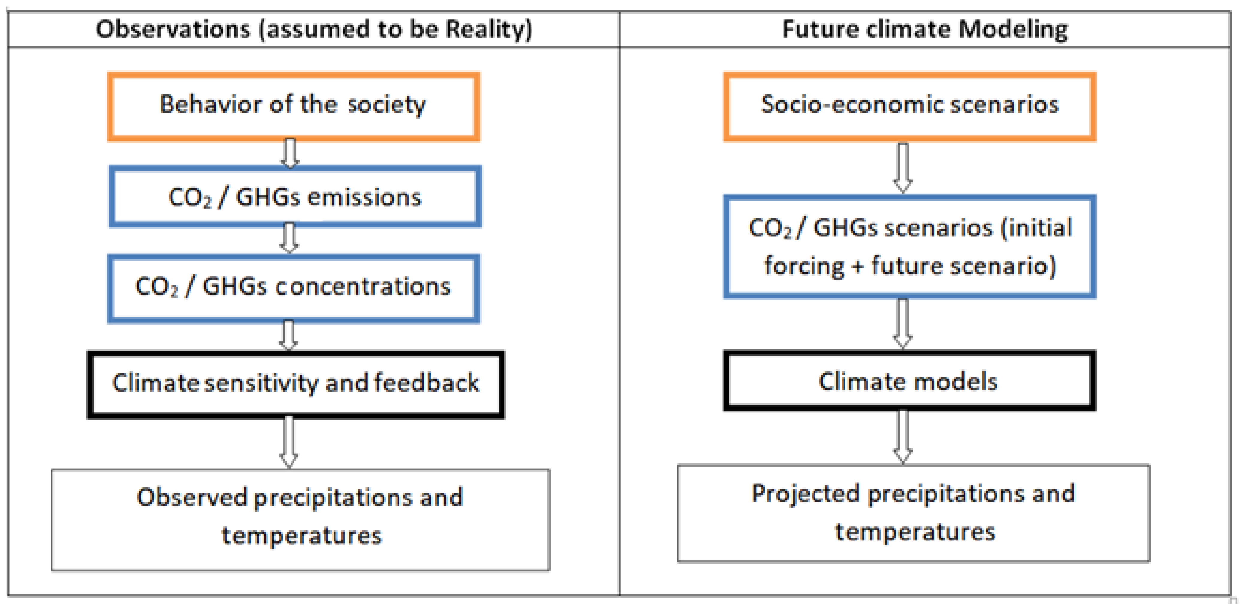
There are many factors influencing the quality of climate models outputs. When considering the current practice in climate modeling science, we have identified three factors we would want to focus on. They are featured in Figure 14, they are socio-economic scenarios, CO2 and other GHGs concentration scenarios and climate model uncertainty.
The results obtained from the models combine uncertainties originating from at least these three sources. Here we want to emphasize on the fact that because the task of predicting the impacts of climate change in the future does not depend solely on models or socio-economic/GHGs scenarios, projections carried out in the past should not just be left aside, at least from AR2. In fact, it is noticeable that past works related to the assessment of the impacts of climate change are generally quickly considered outdated in favor of new sets of socio-economic scenarios; GHGs scenarios; and climate models. These past projections might, however, bring some very useful insight for the future. They offer a unique possibility to verify 25 to 30 years (1990 to present) of past climate predictions. Indeed, Johns et al. [57] provided evidence that ability to reproduce the past record does not necessarily guarantee that predictions of future climate will also be accurate. Next, for the near future, past socio-economic scenarios; past GHGs scenarios; and past models could be evaluated over 1990–2016 and then combined with new socio-economic scenarios, GHGs concentrations and models; depending on the sub-region (See Table 11).
4. Concluding Remarks
The research proposed an approach that intended to learn from the recent past in order to be better prepared for the near future and even for longer terms. Although AR1 projections were not good over WA mainly because of physical parametrizations and spatial resolution of the GISS model, AR2 and AR3 provided, to some extent, valuable results. The most recent models (AR2 and AR3) showed very appreciable performance regarding the climatology, the seasonality and trends. We now have a better insight into how past models and scenarios were able to predict various characteristics of today’s climate. The results can be further analyzed in order to provide a valuable prediction of precipitation and temperature for the next 20–30 years. In fact, one could select, as explained before, a combination of past and new scenarios and models that suit the most specific locations and purposes. Then, results from these runs could be used as short-term projections. We think this approach can become complementary to current climate impact assessments studies.
The observational products used are derived from ground measurements. Knowing the sparse meteorological network and the lack of long-term measurements in WA, we acknowledge that the historical data might present some quality issues especially for precipitation. This WA context makes the evaluation of climate simulations much more difficult than for other geographical regions of the world [71]. Efforts are being made to improve data collection in WA in both quality and quantity, such as the WASCAL (West African Science Service Centre on Climate Change and Adapted Land Use) Hydrometeorological Observatory in the Sudan Savanna of Burkina Faso and Ghana [82]. Recently, in the year 2020, additional equipment has been acquired and added to this regional network.
Another limitation is the fact that our study made use of only 6 datasets, but more or all datasets available from the IPCC data center can be tested in the future, and further studies could consider ensemble- analysis and include analysis of extremes. Basically, new studies could consider comparison of ensembles while the present study just compared one projection to another. We did not consider bias correction of models’ outputs. This is an interesting point to include in next studies. As new climate projections are constantly being developed, we believe an automation of our research methodology could allow us to integrating new observations as time goes by and more recent projections. In fact, we stopped at 2016, but new datasets would go beyond and allow us to work with datasets that span longer than 30 years.
Further studies could be conducted to analyze to what extent some projections might be used for short-term predictions for specific regions and/or applications and what range of uncertainty can be expected. With a larger number of input datasets, certain projections could be identified as more appropriate for a specific region and purpose and then proposed for an ensemble analysis. Such an investigation could be helpful in determining areas where developing models and scenarios will be most profitable.
We expect our study to be useful in complementing classical approaches. Classical approaches do not use previous projections to predict the future. Researchers generally generate new projections based on newer scenarios and models.
We can link the results to various key development sectors. For example, in terms of water resources availability (management purposes), an underestimation of precipitation is preferable to an overestimation, but it would be ideal if the result was as accurate as possible. In the case of preparation against extreme events (floods, droughts), an overestimation of precipitation is desirable for long-term flood risk; and an underestimation is desirable for drought prediction. For agricultural purposes, an analysis of the seasonal cycle, timing, and amplitude of precipitation may be relevant. When related to ecology, some aspects such as the seasonal cycle, timing of precipitation and temperature may be taken into consideration. The elaboration of safety measures in health may be supported by the analysis of seasonal cycles, timing, and values of temperatures; this may be relevant for predicting occurrences of certain vector-borne diseases such as malaria. Other sectors such as farming, fishing, and mobility may also be considered. Further steps could be to use more projection datasets in the analysis and determine to what extent the observed difference is acceptable depending on the sector and the country.
We expect to communicate our research with stakeholders and policy makers in WA via regional and national research and governmental institutions, non-novernmental organizations (NGOs), and possibly the private sector.
Supplementary Materials
The following supporting information can be downloaded at: https://www.mdpi.com/article/10.3390/su141912093/s1.
Author Contributions
Conceptualization, O.U.C.G. and B.D.; methodology, O.U.C.G.; software, O.U.C.G. and Y.U.G.; validation, O.U.C.G. and B.D.; formal analysis, O.U.C.G.; investigation, O.U.C.G.; resources, O.U.C.G., Y.U.G. and B.D.; data curation, O.U.C.G.; writing—original draft preparation, O.U.C.G.; writing—review and editing, O.U.C.G., Y.U.G. and B.D.; visualization, O.U.C.G. and Y.U.G.; supervision, B.D.; project administration, O.U.C.G. and B.D.; funding acquisition, O.U.C.G. and B.D. All authors have read and agreed to the published version of the manuscript.
Funding
The research paper presents a part of the results of the investigations undertaken in the framework of the COMO Project (Comparison of Climate Models and Observations). This project was designed and conducted under the International Climate Protection Fellowship (ICP) scheme which is a research fellowship of the German Alexander von Humboldt Foundation (AvH). This research and APC were funded by the Alexander von Humboldt Foundation within the previously specified context.
Institutional Review Board Statement
Not applicable.
Informed Consent Statement
Not applicable.
Data Availability Statement
The data presented in this study are openly available. The details on where to find the data is given in the Section “Materials and Methods” of this article.
Acknowledgments
The work was carried out under the International Climate Protection Fellowship (ICP) provided by the German Alexander von Humboldt Foundation (AvH), in partnership with the University of Bonn, Germany and the University of Abomey-Calavi, Benin. This paper and the research behind it would not have been possible without their exceptional support. YUG wants to acknowledge that this publication was made possible by a grant from Carnegie Corporation of New York (provided through the African Institute for Mathematical Sciences). The statements made and views expressed are solely the responsibility of the author. The authors also want to express their gratitude to the Deutsches Klimarechenzentrum (DKRZ)—German Climate Computing Centre with special thanks addressed to Franck Toussaint, Michael Böttinger and Ilse Hamann. We are grateful to the West African Science Service Centre on Climate Change and Adapted Land Use (WASCAL) Competence Center (Burkina Faso) in particular to Aymar Bossa, Mouhamadou Bamba SYLLA for their helpful suggestions in the collection of past datasets. We acknowledge the online “cdo” support Team of the Max Planck Institute for Meteorology, Germany for the assistance provided to read some of the past datasets. We also acknowledge the NOAA/OAR/ESRL PSL, Boulder, Colorado, USA for making GHCN Gridded V2 data available from their Web site at https://psl.noaa.gov/ (accessed on 15 October 2019).The authors thank Thomas Poméon for their expertise and assistance in discussing the methodology and writing the codes. The authors want to thank Odou Thierry for his contribution in the creation of the code for the plotting of the Hovmöller diagrams. We are grateful for the insightful comments given by the anonymous peer reviewers at MDPI Open Access Journals. We are also grateful to Andrew Manoba Limantol, Lecturer at the University of Environment and Sustainable Development (UESD), Ghana for his help in proofreading some parts of the manuscript.
Conflicts of Interest
The authors declare no conflict of interest. The funders had no role in the design of the study; in the collection, analyses, or interpretation of data; in the writing of the manuscript; or in the decision to publish the results.
References
- Streimikiene, D. Environmental indicators for the assessment of quality of life. Intellect. Econ. 2015, 9, 67–79. [Google Scholar] [CrossRef]
- IPCC. Intergovernmental Panel on Climate Change (IPCC) Climate Change 2014: Synthesis Report. In Contribution of Working Groups I, II and III to the Fifth Assessment Report of the Intergovernmental Panel on Climate Change; The Core Writing Team, Pachauri, R.K., Meyer, L.A., Eds.; IPCC: Geneva, Switzerland, 2014. [Google Scholar]
- Solomon, S.; Qin, D.; Manning, M.; Chen, Z.; Marquis, M.; Averyt, K.B.; Tignor, M.; Miller, H.L. (Eds.) IPCC Summary for Policymakers. In Climate Change 2007: The Physical Science Basis. Contribution of Working Group I to the Fourth Assessment Report of the Intergovernmental Panel on Climate Change; Cambridge University Press: Cambridge, UK, 2007; pp. 1–18. [Google Scholar]
- Intergovernmental Panel on Climate Change (IPCC) Climate Change 2007: The Physical Science Basis. In Contribution of Working Group I to the Fourth Assessment Report of the Intergovernmental Panel on Climate Change; Solomon, S.; Qin, D.; Manning, M.; Chen, Z.; Marquis, M.; Averyt, K.; Tignor, M.; Miller, H.L. (Eds.) Cambridge University Press: Cambridge, UK; New York, NY, USA, 2007; ISBN 9780521880091. [Google Scholar]
- IPCC Working Group, I. Climate Change 2001: The Scientific Basis. Contribution of Working Group I to the Third Assessment Report of the Intergovernmental Panel on Climate Change; Houghton, J.T., Ding, Y., Griggs, D.J., Noguer, M., van der Linden, P.J., Dai, X., Maskell, K., Johnson, C.A., Eds.; Cambridge University Press: Cambridge, UK; New York, NY, USA, 2001. [Google Scholar]
- Zhang, T.; Gregory, K.; Hammack, R.W.; Vidic, R.D. IPCC Climate Change 1995: A report of the Intergovernmental Panel on Climate Change. Environ. Sci. Technol. 1996, 48, 4596–4603. [Google Scholar] [CrossRef]
- Intergovernmental Panel on Climate Change (IPCC) Climate Change:The 1990 and 1992 IPCC Assessments. In IPCC First Assessment Report. Overview and Policymaker Summaries and 1992 IPCC Supplement; Intergovernmental Panel on Climate Change (IPCC) (Ed.) Intergovernmental Panel on Climate Change (IPCC): Geneva, Switzerland, 1992. [Google Scholar]
- Leggett, J.; Pepper, W.; Swart, R.; Edmonds, J.; Meira Filho, L.; Mintzer, I.; Wang, M. Emissions scenarios for the IPCC: An update. In Climate change 1992. The Supplementary Report to the IPCC Scientific Assessment; Houghton, J., Callander, B., Varney, S.K., Eds.; Cambridge University Press: Cambridge, UK, 1992; pp. 68–95. [Google Scholar]
- United Nations. United Nations United Nations Framework Convention on Climate Change—UNFCCC; UN: Rio de Janeiro, Brazil, 1992. [Google Scholar]
- Sylla, M.B.; Giorgi, F.; Coppola, E.; Mariotti, L. Uncertainties in daily rainfall over Africa: Assessment of gridded observation products and evaluation of a regional climate model simulation. Int. J. Climatol. 2013, 33, 1805–1817. [Google Scholar] [CrossRef]
- Gbobaniyi, E.; Sarr, A.; Sylla, M.B.; Diallo, I.; Lennard, C.; Dosio, A.; Diedhiou, A.; Kamga, A.; Klutse, N.A.B.; Hewitson, B.; et al. Climatology, annual cycle and interannual variability of precipitation and temperature in CORDEX simulations over West Africa. Int. J. Climatol. 2014, 34, 2241–2257. [Google Scholar] [CrossRef]
- Biao, E.I.; Alamou, E.A. Influence of the Long-Range Dependence in Rainfall in Modelling Oueme River Basin (Benin, West Africa). Atmos. Ocean. Sci. 2016, 1, 19–28. [Google Scholar] [CrossRef]
- Alamou, E.A.; Quenum, G.M.L.D.; Lawin, E.A.; Badou, F.D.; Afouda, A. Variabilité spatio-temporelle de la pluviométrie dans le bassin de l’Ouémé, Bénin. Afrique Sci. 2016, 12, 315–328. [Google Scholar]
- N’Tcha M’Po, Y. Comparison of Daily Precipitation Bias Correction Methods Based on Four Regional Climate Model Outputs in Ouémé Basin, Benin. Hydrology 2016, 4, 58. [Google Scholar] [CrossRef]
- Klutse, N.A.B.; Sylla, M.B.; Diallo, I.; Sarr, A.; Dosio, A.; Diedhiou, A.; Kamga, A.; Lamptey, B.; Ali, A.; Gbobaniyi, E.O.; et al. Daily characteristics of West African summer monsoon precipitation in CORDEX simulations. Theor. Appl. Climatol. 2016, 123, 369–386. [Google Scholar] [CrossRef]
- Sylla, M.B.; Elguindi, N.; Giorgi, F.; Wisser, D. Projected robust shift of climate zones over West Africa in response to anthropogenic climate change for the late 21st century. Clim. Change 2016, 134, 241–253. [Google Scholar] [CrossRef]
- Klein, C.; Bliefernicht, J.; Heinzeller, D.; Gessner, U.; Klein, I.; Kunstmann, H. Feedback of observed interannual vegetation change: A regional climate model analysis for the West African monsoon. Clim. Dyn. 2017, 48, 2837–2858. [Google Scholar] [CrossRef]
- Heinzeller, D.; Dieng, D.; Smiatek, G.; Olusegun, C.; Klein, C.; Hamann, I.; Salack, S.; Bliefernicht, J.; Kunstmann, H. The WASCAL high-resolution regional climate simulation ensemble for West Africa: Concept, dissemination and assessment. Earth Syst. Sci. Data 2018, 10, 815–835. [Google Scholar] [CrossRef] [Green Version]
- Abroulaye, S.; Issa, S.; Abalo, K.E.; Nouhoun, Z. Climate Change: A Driver of Crop Farmers-Agro Pastoralists Conflicts in Burkina Faso. Int. J. Sci. Technol. 2015, 5, 92–104. [Google Scholar]
- Koudamiloro, O.; Vissin, E.W.; Sintondji, L.O.; Houssou, C.S. Risques hydroclimatiques dans le bassin versant du fleuve Ouémé à l’exutoire de Bétérou au Bénin (Afique de l’ouest). XXVIIIe Colloq. l’Association Int. Climatol. 2015, 543–548. Available online: https://docplayer.fr/29392349-Xxviiie-colloque-de-l-association-internationale-de-climatologie-liege-2015.html (accessed on 11 September 2022).
- Amoussou, E.; Vodounon, H.T.; Sourou, H.; Allagbe, S.; Kodja, J.D.; Akognongbe, A.; Sohou, B.; Expédit, E.V.; Boko, M.; Houndenou, C.; et al. Péjoration climatique et dynamique hydroécologique dans le bassin-versant du fleuve Ouémé à Bonou au Bénin. Hydrol. Sci. J. 2015, 57, 235–244. [Google Scholar]
- Kabore/Bontogho, T.-N.P.E.; Ibrahim, B.; Barry, B.; Helmschrot, J. Intra-Seasonal Variability of Climate Change in Central Burkina Faso. Int. J. Curr. Eng. Technol. 2015, 5, 1955–1965. [Google Scholar]
- Yéo, W.E.; Goula, B.T.A.; Diekkrüger, B.; Afouda, A. Vulnerability and adaptation to climate change in the Comoe River Basin (West Africa). Springerplus 2016, 5, 15. [Google Scholar] [CrossRef] [PubMed]
- Project RAPSAHEL. Cartographie de la Vulnérabilité des Ecosystèmes et des Populations aux Changements Climatiques en Afrique de L’ouest: Approche Opérationnelle Pour L’élaboration des Cartes de Vulnérabilités. 2017. Available online: https://www.researchgate.net/publication/332242436_Etat_de_l’art_sur_la_vulnerabilite_des_ecosystemes_et_des_populations_aux_changements_climatiques_en_Afrique_de_l’Ouest_une_revue_bibliographique_et_cartographique (accessed on 28 November 2020).
- Badou, F.; Kapangaziwiri, E.; Diekkrüger, B.; Hounkpe, J.; Afouda, A. Evaluation of recent hydro-climatic changes in four tributaries of the Niger river Basin (West Africa). Hydrol. Sci. J. 2017, 62, 715–728. [Google Scholar] [CrossRef]
- Labitan, C.; Totin, E.; Segnon, A.; D’haen, S. État des Lieux des Connaissances Scientifiques Actuelles sur les Impacts, la Vulnérabilité, et L’adaptation aux Changements Climatiques au Bénin; Adaptation Community: Cotonou, Benin, 2018. [Google Scholar]
- Jung, G.; Wagner, S.; Kunstmann, H. Joint climate-hydrology modeling: An impact study for the data-sparse environment of the Volta Basin in West Africa. Hydrol. Res. 2012, 43, 231–248. [Google Scholar] [CrossRef]
- Sylla, M.B.; Pal, J.S.; Wang, G.L.; Lawrence, P.J. Impact of land cover characterization on regional climate modeling over West Africa. Clim. Dyn. 2016, 46, 637–650. [Google Scholar] [CrossRef]
- Obada, E.; Alamou, E.A.; Zandagba, J.; Chabi, A.; Afouda, A. Change in future rainfall characteristics in the Mekrou catchment (Benin), from an ensemble of 3 RCMs (MPI-REMO, DMI-HIRHAM5 and SMHI-RCA4). Hydrology 2017, 4, 14. [Google Scholar] [CrossRef]
- Sylla, M.B.; Faye, A.; Giorgi, F.; Diedhiou, A.; Kunstmann, H. Projected Heat Stress Under 1.5 °C and 2 °C Global Warming Scenarios Creates Unprecedented Discomfort for Humans in West Africa. Earth’s Future 2018, 6, 1029–1044. [Google Scholar] [CrossRef]
- Ministry of Environment-Benin. Communication Nationale Initiale du Bénin sur les Changements Climatiques; Projet BEN/98/G31 «Changements Climatiques»; Ministry of Environment-Benin: Cotonou, Benin, 2001.
- Gouvernment of Burkina Faso. Communication Nationale du Burkina Faso; Gouvernment of Burkina Faso: Ouagadougou, Burkina Faso, 2001.
- Ministry of Environment-CI. Communication Nationale Initiale de la Côte d’Ivoire; Ministry of Environment-CI: Abidjan, Côte d’Ivoire, 2000.
- Department of State for Environment-The Gambia. First National Communication of the Republic of the Gambia To the United Nations Framework Convention on Climate Change; Department of State for Environment-The Gambia: Banjul, The Gambia, 2003.
- Environmental Protection Agency-Ghana. Ghana’s Second National Communication to the UNFCCC; Environmental Protection Agency-Ghana: Accra, Ghana, 2011. [Google Scholar]
- Ministry of Environment-Guinea. Communication Initiale de la Guinée à la Convention Cadre des Nations Unies sur les Changements Climatiques; Ministry of Environment-Guinea: Conakry, Guinea, 2002.
- Environmental Protection Agency-Liberia. Initial National Communication; Monrovia, Liberia, 2013. Environmental Protection Agency-Liberia: Monrovia, Liberia, 2013. [Google Scholar]
- Ministry of Environment-Mali. Convention Cadre de Nation Unies sur les Changements Climatiques: Communication Initiale du Mali; Ministry of Environment-Mali: Bamako, Mali, 2000.
- National Council of Environment-Niger. Seconde Communication Nationale du Niger; National Council of Environment-Niger: Niamey, Niger, 2009.
- Federal Ministry of Environment Abuja. Nigeria’s Second National Communication; Federal Ministry of Environment Abuja: Abuja, Nigeria, 2014.
- Ministry of Environment-Togo. Communication Nationale Initiale du Togo; Ministry of Environment-Togo: Lomé, Togo, 2001.
- Wilby, R.L.; Dessai, S. Robust adaptation to climate change. Weather 2010, 65, 180–185. [Google Scholar] [CrossRef]
- Rahmstorf, S.; Foster, G.; Cazenave, A. Comparing climate projections to observations up to 2011. Environ. Res. Lett. 2012, 7, 044035. [Google Scholar] [CrossRef]
- Singh, B.B.; Kumar, K.N.; Seelanki, V.; Karumuri, R.K.; Attada, R.; Kunchala, R.K. How reliable are Coupled Model Intercomparison Project Phase 6 models in representing the Asian summer monsoon anticyclone? Int. J. Climatol. 2022, 1–13. [Google Scholar] [CrossRef]
- Reifen, C.; Toumi, R. Climate projections: Past performance no guarantee of future skill? Geophys. Res. Lett. 2009, 36, 1–5. [Google Scholar] [CrossRef] [Green Version]
- Hausfather, Z. Analysis: How Well Have Climate Models Projected Global Warming? Carbon Brief. 2017. Available online: https://www.carbonbrief.org/analysis-how-well-have-climate-models-projected-global-warming. (accessed on 23 April 2020).
- Kahn, B. Exxon Predicted 2019’s Ominous CO2 Milestone in 1982. Earther Gizmodo. 2019. Available online: https://gizmodo.com/exxon-predicted-2019-s-ominous-co2-milestone-in-1982-1834748763 (accessed on 23 April 2020).
- Schneider, U.; Becker, A.; Finger, P.; Meyer-Christoffer, A.; Ziese, M. GPCC Full Data Monthly Product Version 2018 at 0.25°: Monthly Land-Surface Precipitation from Rain-Gauges built on GTS-based and Historical Data. Glob. Precip. Climatol. Cent. 2018. [Google Scholar] [CrossRef]
- Poméon, T.; Jackisch, D.; Diekkrüger, B. Evaluating the performance of remotely sensed and reanalysed precipitation data over West Africa using HBV light. J. Hydrol. 2017, 547, 222–235. [Google Scholar] [CrossRef]
- Fan, Y.; van den Dool, H. A global monthly land surface air temperature analysis for 1948-present. J. Geophys. Res. Atmos. 2008, 113, 1–18. [Google Scholar] [CrossRef]
- Website SRES Emissions Scenarios. Data Distribution Center of the IPCC. 2019. Available online: https://sedac.ciesin.columbia.edu/ddc/sres/index.html (accessed on 13 June 2019).
- Hansen, J.; Russell, G.; Rind, D.; Stone, P.; Lacis, A.; Lebedeff, S.; Ruedy, R.; Travis, L. Efficient three-dimensional global models for climate studies: Models I and II. Mon. Weather Rev. 1983, 111, 609–662. [Google Scholar] [CrossRef]
- (NASA/GISS), N.G.I. for S.S. IPCC-DDC FAR GISS SCENARIO A 2008; World Data Center for Climate (WDCC) at DKRZ: Hamburg, Germany, 2008. [Google Scholar]
- (NASA/GISS), N.G.I. for S.S. IPCC-DDC FAR GISS SCENARIO B 2008; World Data Center for Climate (WDCC) at DKRZ: Hamburg, Germany, 2008.
- Dixon, K.W.; Delworth, T.L.; Knutson, T.R.; Spelman, M.J.; Stouffer, R.J. A comparison of climate change simulations produced by two GFDL coupled climate models. Glob. Planet. Change 2003, 37, 81–102. [Google Scholar] [CrossRef]
- Stouffer, R.J. GF01GG01-GHG: THE 100-YEAR GREENHOUSE GAS INTEGRATION of GFDL 2001. World Data Center for Climate (WDCC) at DKRZ. 2001. Available online: https://www.wdc-climate.de/ui/entry?acronym=GF01GG01 (accessed on 18 June 2019).
- Johns, T.C.; Carnell, R.E.; Crossley, J.F.; Gregory, J.M.; Mitchell, J.F.B.; Senior, C.A.; Tett, S.F.B.; Wood, R.A. The second Hadley Centre coupled ocean-atmosphere GCM: Model description, spinup and validation. Clim. Dyn. 1997, 13, 103–134. [Google Scholar] [CrossRef]
- Mitchell, J. HC01GS01-GSG:The Sulphate Aerosol and Greenhouse Gas Integration 2001; World Data Center for Climate (WDCC) at DKRZ: Hamburg, Germany, 2001. [Google Scholar]
- Johns, T.C.; Gregory, J.M.; Ingram, W.J.; Johnson, C.E.; Jones, A.; Lowe, J.A.; Mitchell, J.F.B.; Roberts, D.L.; Sexton, D.M.H.; Stevenson, D.S.; et al. Anthropogenic climate change for 1860 to 2100 simulated with the HadCM3 model under updated emissions scenarios. Clim. Dyn. 2003, 20, 583–612. [Google Scholar] [CrossRef]
- Johns, T.C.; Gregory, J.M.; Ingram, W.J.; Johnson, C.E.; Jones, A.; Lowe, J.A.; Mitchell, J.F.B.; Roberts, D.L.; Sexton, D.M.H.; Stevenson, D.S.; et al. IPCC-DDC_HADCM3_SRES_A2: 150 YEARS MONTHLY; MEANS Hadley Centre for Climate Prediction and Research-UK Met Office, World Data Center for Climate (WDCC) at DKRZ: Hamburg, Germany, 2004. [Google Scholar] [CrossRef]
- Johns, T.C.; Gregory, J.M.; Ingram, W.J.; Johnson, C.E.; Jones, A.; Lowe, J.A.; Mitchell, J.F.B.; Roberts, D.L.; Sexton, D.M.H.; Stevenson, D.S.; et al. IPCC-DDC_HADCM3_SRES_B2: 150 YEARS MONTHLY; MEANS Hadley Centre for Climate Prediction and Research-UK Met Office, World Data Center for Climate (WDCC) at DKRZ: Hamburg, Germany, 2004. [Google Scholar]
- Wayne, G. The Beginner’s Guide to Representative Concentration Pathways By Skeptical Science By Skeptical Science. 2013. Available online: https://skepticalscience.com/doc (accessed on 31 October 2019).
- IPCC Working Group I. Climate Change: The IPCC Scientific Assesment; Houghton, J.T., Jenkins, G.J., Ephraums, J.J., Eds.; Cambridge University Press: Cambridge, UK, 1990. [Google Scholar]
- IPCC Working Group III. Climate Change: The IPCC Response Strategies; Bernthal, F., Dowdeswell, E., Luo, J., Attard, D., Vellinga, P., Karimanzira, R., Eds.; Cambridge University Press: Cambridge, UK, 1990. [Google Scholar]
- van Vuuren, D.P.; Edmonds, J.; Kainuma, M.; Riahi, K.; Thomson, A.; Hibbard, K.; Hurtt, G.C.; Kram, T.; Krey, V.; Lamarque, J.F.; et al. The representative concentration pathways: An overview. Clim. Change 2011, 109, 5–31. [Google Scholar] [CrossRef]
- Bjørnæs, C. A Guide to Representative Concentration Pathways. CICERO Center. 2015. Available online: https://cicero.oslo.no/en/posts/news/a-guide-to-representative-concentration-pathways (accessed on 5 November 2019).
- Girod, B.; Wiek, A.; Mieg, H.; Hulme, M. The evolution of the IPCC’s emissions scenarios. Environ. Sci. Policy 2009, 12, 103–118. [Google Scholar] [CrossRef]
- Intergovernmental Panel on Climate Change (IPCC). Climate Change 2021: The Physical Science Basis. Contribution of Working Group I to the Sixth Assessment Report of the Intergovernmental Panel on Climate Change; Masson-Delmotte, V., Zhai, P., Pirani, A., Connors, S.L., Péan, C., Berger, S., Caud, N., Chen, Y., Goldfarb, L., Gomis, M.I., et al., Eds.; In press; Cambridge University Press: Cambridge, UK; New York, NY, USA, 2021. [Google Scholar]
- Di Liberto, T. Hovmöller Diagram: A Climate Scientist’s Best Friend. ClimateWatch Magazine NOAA Cliamte.gov. 2020. Available online: https://www.climate.gov/news-features/understanding-climate/hovmöller-diagram-climate-scientist’s-best-friend (accessed on 12 October 2020).
- Comité Permanent Inter-états de Lutte contre la Sécheresse dans le Sahel (CILSS). Landscapes of West Africa—A Window on a Changing World; Comité Permanent Inter-états de Lutte contre la Sécheresse dans le Sahel (CILSS): Ouagadougou, Burkina Faso, 2016. Available online: https://eros.usgs.gov/westafrica (accessed on 12 October 2020).
- Dieng, D.; Smiatek, G.; Bliefernicht, J.; Heinzeller, D.; Sarr, A.; Gaye, A.T.; Kunstmann, H. Evaluation of the COSMO-CLM high-resolution climate simulations over West Africa. J. Geophys. Res. 2017, 122, 1437–1455. [Google Scholar] [CrossRef]
- Ibrahim, B. Caractérisation des Saisons de Pluies au Burkina Faso dans un Contexte de Changement Climatique et Évaluation des Impacts Hydrologiques sur le Bassin du Nakanbé. Doctoral Thesis, Université Pierre et Marie Curie (UPMC) & Institut International d’Ingénierie de l’Eau et de l’Environnement (2iE), Paris, France, 2012. [Google Scholar]
- Sultan, B.; Janicot, S. The West African Monsoon Dynamics. Part II: The ‘“ Preonset ”’ and “ Onset ” of the Summer Monsoon. J. Clim. 2003, 16, 3407–3427. [Google Scholar] [CrossRef]
- Hulme, M.; Doherty, R.; Ngara, T.; New, M.; Lister, D. African climate change: 1900–2100. Clim. Res. 2001, 17, 145–168. [Google Scholar] [CrossRef]
- Gaba, O.U.; Poméon, T.; Diekkrueger, B.; Gaba, Y.U. How good have our climate models been so far ? A case study from West Africa. In Proceedings of the EGU General Assembly 2020, Online, 4–8 May 2020. [Google Scholar] [CrossRef]
- Akinseye, F.M.; Agele, S.O.; Traore, P.C.S.; Adam, M.; Whitbread, A.M. Evaluation of the onset and length of growing season to define planting date—‘A case study for Mali (West Africa )’. Theor. Appl. Climatol. 2016, 124, 973–983. [Google Scholar] [CrossRef]
- Sultan, B.; Janicot, S. Abrupt Shift of the ITCZ over West Africa and intra-seasonal variability over. Geophys. Res. Lett. 2000, 27, 3353–3356. [Google Scholar] [CrossRef]
- Dieng, D.; Smiatek, G.; Heinzeller, D.; Kunstmann, H. Simulation of the Rain Belt of the West African Monsoon (WAM) in High Resolution CCLM Simulation. In High Performance Computing in Science and Engineering; Nagel, W.E., Ed.; Springer International Publishing AG: Berlin/Heidelberg, Germany, 2016; Volume 16, pp. 547–558. ISBN 9783319470665. [Google Scholar]
- Paxian, A.; Sein, D.; Panitz, H.-J.; Warscher, M.; Breil, M.; Engel, T.; Tödter, J.; Krause, A.; Cabos Narvaez, W.D.; Fink, A.H.; et al. Bias reduction in decadal predictions of West African monsoon rainfall using regional climate models. J. Geophys. Res. Atmos. 2016, 119, 1715–1735. [Google Scholar] [CrossRef]
- Intergovernmental Panel on Climate Change (IPCC). Climate Change 2007: Synthesis Report.Contribution of Working Groups I, II and III to the Fourth Assessment Report of the Intergovernmental Panel on Climate Change; The Core Writing Team, Pachauri, R., Reisinger, A., Eds.; IPCC: Geneva, Switzerland, 2007. [Google Scholar]
- Pope, V.D.; Gallani, M.L.; Rowntree, P.R.; Stratton, R.A. The impact of new physical parametrizations in the Hadley Centre climate model: HadAM3. Clim. Dyn. 2000, 16, 123–146. [Google Scholar] [CrossRef]
- Bliefernicht, J.; Berger, S.; Salack, S.; Guug, S.; Hingerl, L.; Heinzeller, D.; Mauder, M.; Steinbrecher, R.; Steup, G.; Bossa, A.Y.; et al. The WASCAL Hydrometeorological Observatory in the Sudan Savanna of Burkina Faso and Ghana. Vadose Zone J. 2018, 17, 180065. [Google Scholar] [CrossRef] [Green Version]
Figure 1.
Summary of the methodology.

Figure 2.
Bioclimatic Regions of WA. Source: [70].
Figure 2.
Bioclimatic Regions of WA. Source: [70].
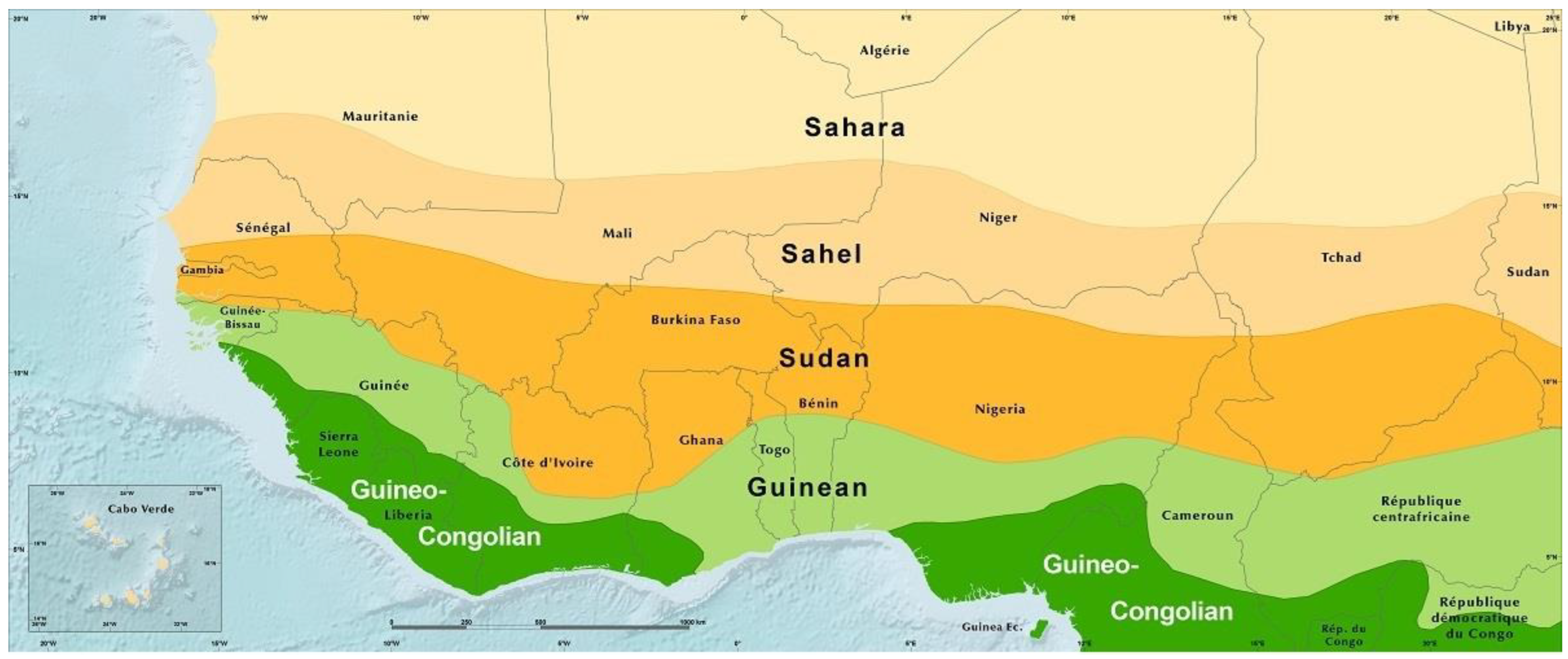
Figure 3.
Definition of Sahel, Soudano and Guinea sub-regions for our study. Taken from Heinzeller et al. [18].
Figure 3.
Definition of Sahel, Soudano and Guinea sub-regions for our study. Taken from Heinzeller et al. [18].
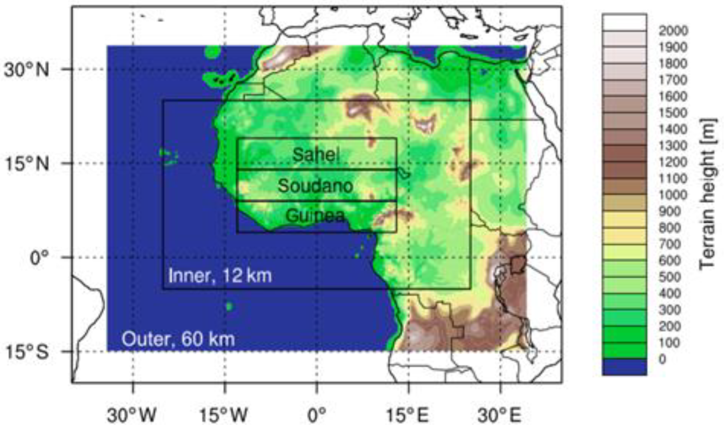
Figure 4.
Mean annual rainfall climatology (mm month−1) for the period 1990–2016 for GPCC observation and each of the past projections. Orographic zones: GH (Guinea Highlands), JP (Jos Plateau) and CM (Cameroun Mountains) are indicated.
Figure 4.
Mean annual rainfall climatology (mm month−1) for the period 1990–2016 for GPCC observation and each of the past projections. Orographic zones: GH (Guinea Highlands), JP (Jos Plateau) and CM (Cameroun Mountains) are indicated.
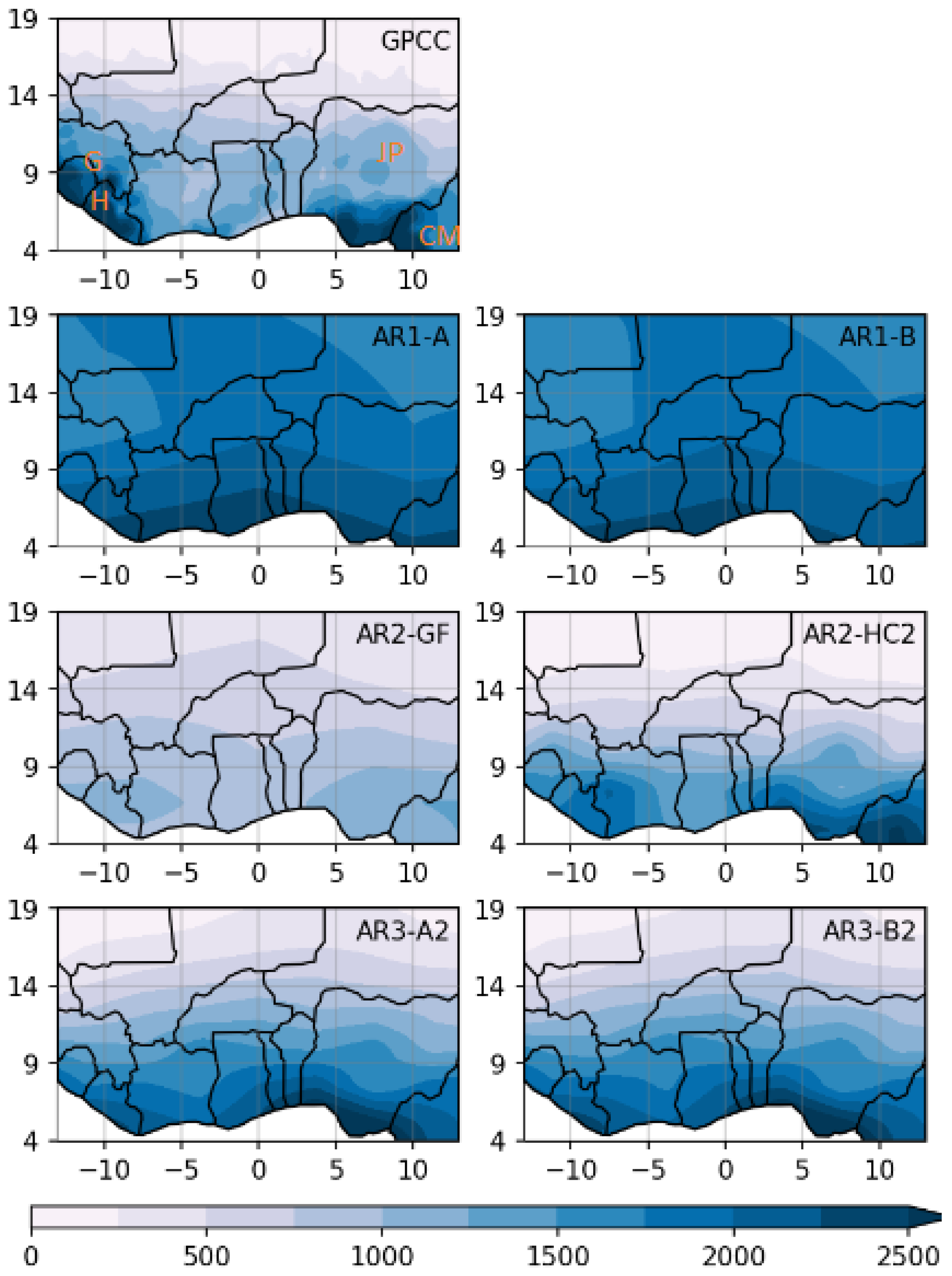
Figure 5.
Percentage of difference in mean rainfall climatology for the period 1990–2016 between each of the past projections and GPCC observation dataset.
Figure 5.
Percentage of difference in mean rainfall climatology for the period 1990–2016 between each of the past projections and GPCC observation dataset.

Figure 6.
Annual cycle of monthly precipitation (mm month−1) averaged over the Sahel, Soudano, Guinea sub-regions and the entire WA and for the period 1990–2016 for GPCC observation and each of the past projections.
Figure 6.
Annual cycle of monthly precipitation (mm month−1) averaged over the Sahel, Soudano, Guinea sub-regions and the entire WA and for the period 1990–2016 for GPCC observation and each of the past projections.
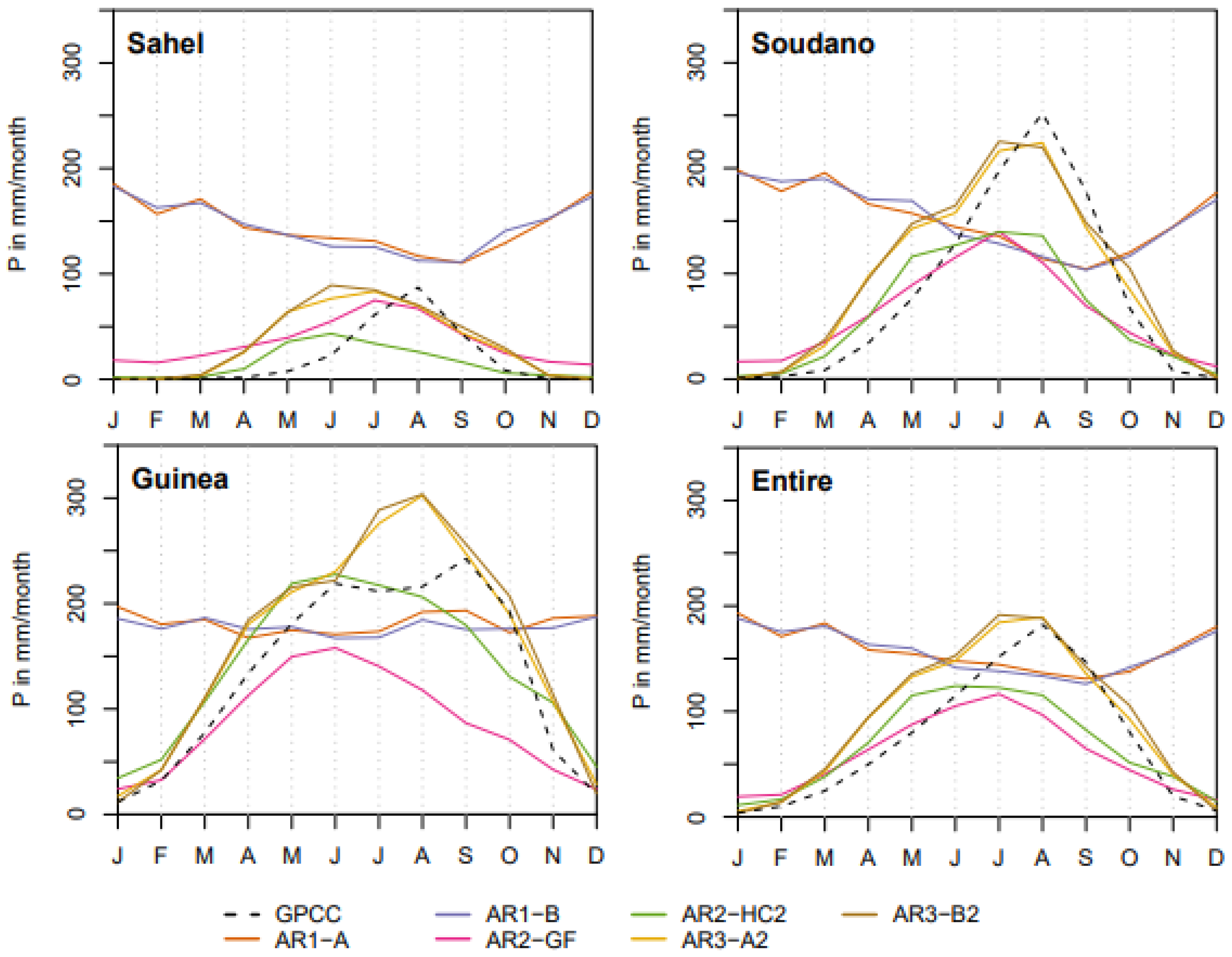
Figure 7.
Hovmöller diagram of monthly precipitation (mm month−1) averaged between 13° W and 13° E and for the period 1990–2016 for GPCC observations and each of the past projections.
Figure 7.
Hovmöller diagram of monthly precipitation (mm month−1) averaged between 13° W and 13° E and for the period 1990–2016 for GPCC observations and each of the past projections.

Figure 8.
Trends of annual precipitation (mm year−1) averaged over the Sahel, Soudano, Guinea sub-regions and the entire WA for the period 1950–2100 for GPCC observation and each of the past projections.
Figure 8.
Trends of annual precipitation (mm year−1) averaged over the Sahel, Soudano, Guinea sub-regions and the entire WA for the period 1950–2100 for GPCC observation and each of the past projections.

Figure 9.
Mean temperature climatology (°C) for the period 1990–2016 for GHCN-CAMS observation and each of the past projections.
Figure 9.
Mean temperature climatology (°C) for the period 1990–2016 for GHCN-CAMS observation and each of the past projections.

Figure 10.
Percentage of difference in mean temperature climatology for the period 1990–2016 between each of the past projections and GHCN-CAMS observation dataset.
Figure 10.
Percentage of difference in mean temperature climatology for the period 1990–2016 between each of the past projections and GHCN-CAMS observation dataset.

Figure 11.
Annual cycle of monthly temperatures (°C) averaged over the Sahel, Soudano, Guinea sub-regions and the entire WA and for the period 1990–2016 for GHCN-CAMS observation and each of the past projections.
Figure 11.
Annual cycle of monthly temperatures (°C) averaged over the Sahel, Soudano, Guinea sub-regions and the entire WA and for the period 1990–2016 for GHCN-CAMS observation and each of the past projections.
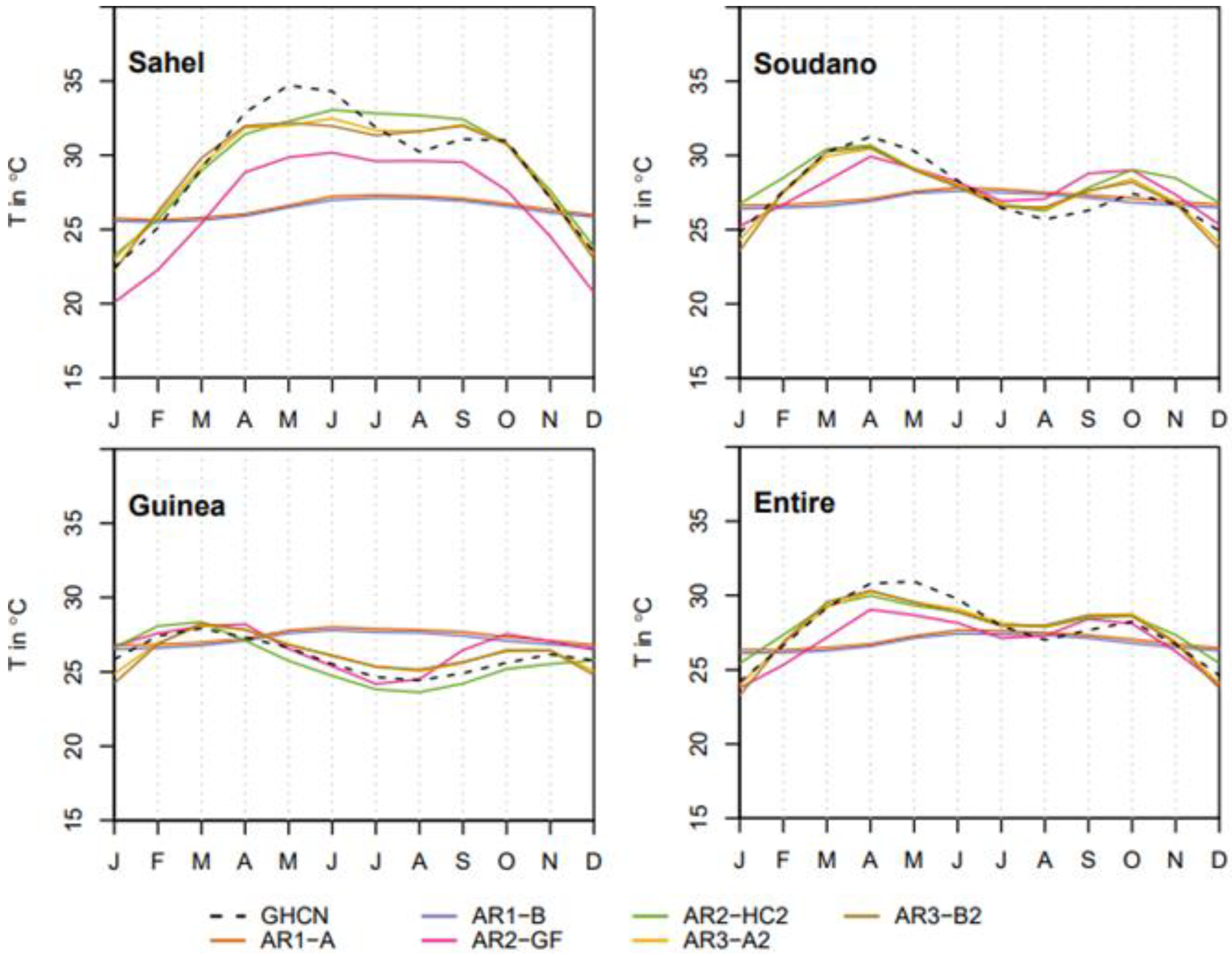
Figure 12.
Hovmöller diagram of monthly temperatures (°C) averaged between 13° W and 13° E and for the period 1990–2016 for GHCN-CAMS observation and each of the past projections.
Figure 12.
Hovmöller diagram of monthly temperatures (°C) averaged between 13° W and 13° E and for the period 1990–2016 for GHCN-CAMS observation and each of the past projections.

Figure 13.
Trends of monthly temperature (°C) averaged over the Sahel, Soudano, Guinea sub-regions and the entire WA for the period 1950–2100 for GHCN-CAMS observation and each of the past projections.
Figure 13.
Trends of monthly temperature (°C) averaged over the Sahel, Soudano, Guinea sub-regions and the entire WA for the period 1950–2100 for GHCN-CAMS observation and each of the past projections.
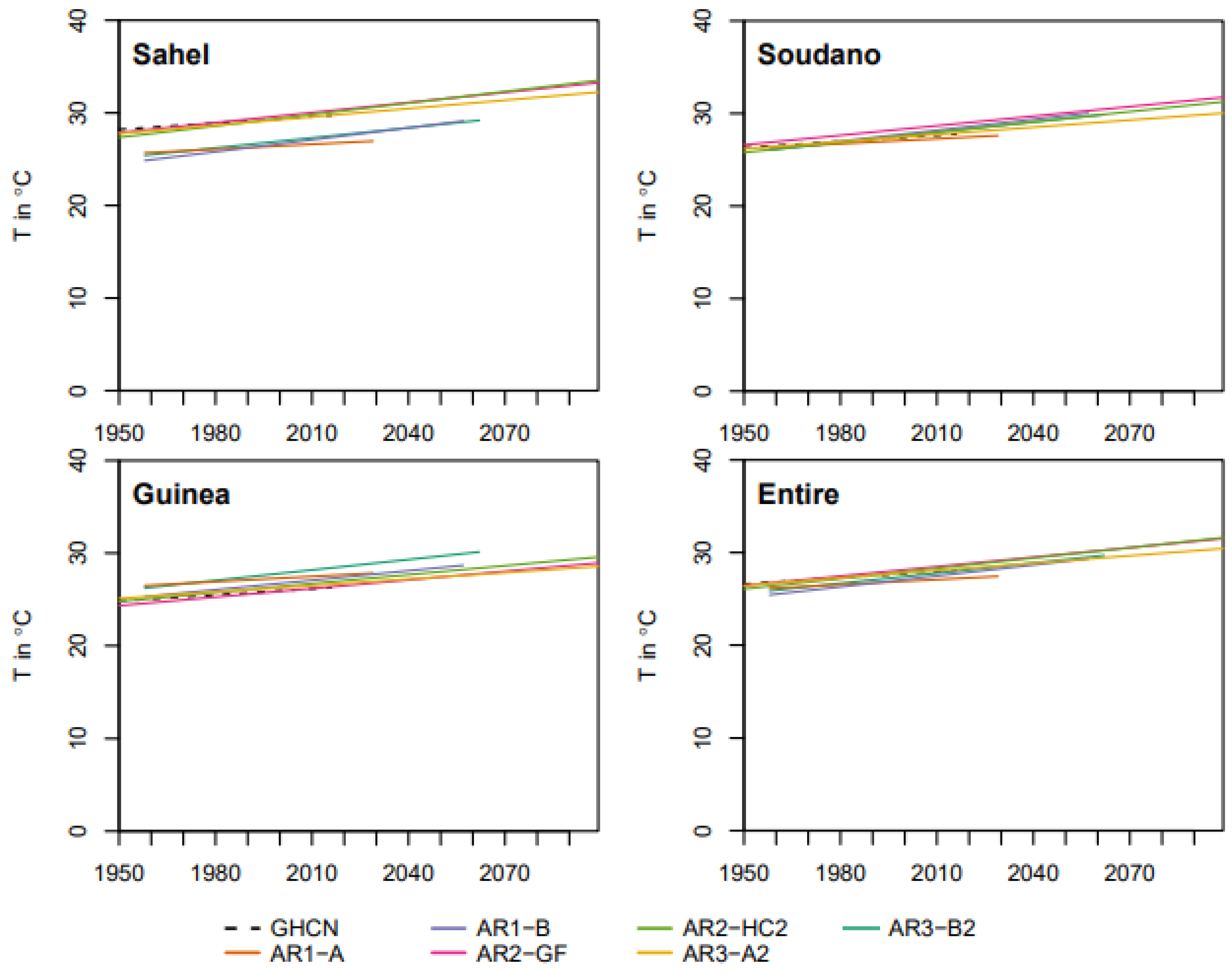
Figure 14.
Identification of some important parameters influencing the quality of future climate change projections.
Figure 14.
Identification of some important parameters influencing the quality of future climate change projections.

Table 1.
A summary of some climate change impacts on temperature and precipitation projected by WA countries in the framework of their National Communications to the UNFCCC.
Table 1.
A summary of some climate change impacts on temperature and precipitation projected by WA countries in the framework of their National Communications to the UNFCCC.
| Study | Models Used and Scenarios | Projected Change | |
|---|---|---|---|
| 1 | Initial National Communication of Benin [31] | MAGICC SCENGEN (ensembles of models), 3 scenarios IS92a (reference scenario); IS92c (optimistic scenario) et IS92e (extreme scenario) from 1990 | ΔT = +0.5 °C by 2025 +1 °C < ΔT < +2.5 °C by 2100 (−30%) < ΔP < +50% (reference 1961–1990) by 2100 |
| 2 | National Communication of Burkina Faso [32] | Japan Meteorological Agency; 2 scenarios (equilibrium and transient at 0.5% annual rate) | ΔT = +0.5 °C by 2025 ΔP < +50% (reference 1961–1995) by 2025 |
| 3 | Initial National Communication of Côte d’Ivoire [33] | GFD3 and UK89 climate models, reference 1994 | +2 °C < ΔT < +4 °C by 2100 UK89: increase of P GFD3: decrease of P |
| 4 | First National communication of the Republic of the Gambia [34] | Seven models were run but 4 were kept for analysis: 1-GFDL (Geophysical Fluid Dynamic Laboratory), 2-CCCM (Canadian Climate Change Model), 3-HCGG (Hadley Centre with Greenhouse Gases (GHGs)), 4-HCGS (Hadley Centre with GHGs and Sulphate aerosol) 1xCO2 and 2xCO2 | +3 °C < ΔT < +4.5 °C by 2075 (−59%) < ΔP < +29% (reference 1951–1990) by 2100 |
| 5 | Ghana’s Second National Communication to the UNFCCC [35] | Hadley Centre Model 2 (HadCM2); UK Meteorological Office Transient Model (UKTR); UK Meteorological Office High Resolution Model (UKHI). Business as usual scenario | Reference: 1961–2000 ΔT = +0.6 °C by 2020 ΔT = +2 °C by 2050 ΔT = +3.9 °C by 2080 Decrease in P 3% by 2020 and 21% by 2080 |
| 6 | Initial Communication of Guinea [36] | Same models as Ghana IS92 | Reference: 1961–1990 +0.2 °C < ΔT < +4.8 °C by 2100 over (2000–2100) Decrease in P that could reach (−40%) by 2100 |
| 7 | Initial National Communication of Liberia [37] | ECHAM5, HadCM3 and 10 RCM A1B scenarios | Reference: 1961–1990 ΔT = +0.4 °C (over 2010–2019) ΔT = +2.6 °C (over 2020–2049) Decrease in P 2% by 2019 and 9.2% by 2049 |
| 8 | Initial Communication of Mali [38] | MAGICC SCENGEN: HadCM2 1xCO2 and 2xCO2 | Reference 1961–1990. 2xCO2: +2.7 °C < ΔT < +4.5 °C by 2025 Decrease in P 10% by 2025 |
| 9 | Second National Communication of Niger [39] | HadCM3: scenarios A2 and B2. CGCM3 (Canadian Centre for Climate Modeling and Analysis): scenarios A2 and B1. MPI-ECHAM5, CSIRO-MK3, GFDL-CGCM2, MRI-CGM2. 1 RCM | Reference 1961–1990. Over 2020–2049: +1.5 °C < ΔT < +2.3 °C (–2%) < ΔP < +50% |
| 10 | Nigeria’s Second National Communication [40] | No clear reference to models used. B1 and A2 scenarios | Reference: 1961–1990. 2050s (2046–2065): +1.8 °C < ΔT < +2.2 °C 2090s (2081–2100): +2.2 °C < ΔT < +4.5 °C |
| 11 | Initial National Communication of Togo [41] | HadCM2, Csiro-Tr (Australia’s Commonwealth Scientific and Industrial Research Organization, Australia), and BMRC-EQ (Australian Bureau of Meteorological Research Center) Scenario IS92a | Reference: 1961–1990 -by 2025 + 0.47% < ΔT < +0.58% (−0.3%) < ΔP < (−0.1%) -by 2050 +1 °C < ΔT < +1.25 °C (−0.8%) < ΔP < (+0.6%) -by 2100 +2.3 °C < ΔT < +2.7 °C (−1.25%) < ΔP < (+1%) |
Table 2.
Characteristics of the Ocean and Atmospheric General Circulation Models (OAGCMs) and scenarios used for the observations-projections comparison.
Table 2.
Characteristics of the Ocean and Atmospheric General Circulation Models (OAGCMs) and scenarios used for the observations-projections comparison.
| IPCC Assessment Reports (AR) | Climate Models. (Lat. × Long.). References | Available Runs | Selected Runs | Period | Sources of Data |
|---|---|---|---|---|---|
| AR1, 1990 | Goddard Institute for Space Studies (GISS). USA. (7.830 × 100). [52] | Control Scenario A Scenario B Equilibrium | Scenario A:“Business-as-Usual (BaU)”. It was run in the mid-1980s. | 1958–2062 | National Aeronautics and space Administration [53] |
| Scenario B: the 2060 Low Emissions Scenario. It was run in the mid-1980s. | 1958–2029 | [54] | |||
| AR2, 1995 | Geophysical Fluid Dynamics Laboratory (GFDL-R30). USA. (2.250 × 3.750). [55] | Control ghg ghg + s: (ghg and sulphate aerosol) | GHGs—“Business-as-Usual (BaU)”. The value of CO2 increases gradually at the rate of 1% per year from the initial value (approximately equal to the value observed in 1958). | 1958–2058 | [56] |
| AR2, 1995 | Hadley Centre for Climate Prediction and Research (Hadley Centre Coupled Model version 2: HadCM2). UK. (2.50 × 3.750). [57] | Control 1 ensemble of 4 runs: (ghg 1%) 1 ensemble of 4 runs: (ghg 0.5 %) 1 ensemble of 4 runs: (ghg + s 1%) 1 ensemble of 4 runs: (ghg +s 0.5%) | First ensemble member of ghg 1%: (IPCC Scenarios) IS92a (approx. IPCC: “Business-as-Usual (BaU)” scenario). The GHGs forcing is increased gradually to represent the observed changes in forcing due to all the ghg from 1860 to 1990. From 1990 to 2100 it uses a 1% per year compounded increase in concentrations. | 1860–2099 | [58] |
| AR3, 2001 | Hadley Centre for Climate Prediction and Research (Hadley Centre Coupled Model version 3: HadCM3). UK. (2.50 × 3.750). [59] | 1 ensemble of 3 runs: (A2, A2b, A2c) Scenario B2 | Special Report on Emission Scenarios (SRES) A2 storyline: continuous increasing population together with a slower economic growth and technological change | 1950–2099 | [60] |
| Special Report on Emission Scenarios (SRES) B2 storyline: emphasis is put on local solutions to economic, social and environmental sustainability. The global population is increasing at a lower rate than storyline A2. | 1950–2099 | [61] |
Table 3.
Summary of IPCC scenarios used since AR1.
| Year | Name | Used in | Scenarios |
|---|---|---|---|
| 1990 | 1990 IPCC Scenario A: SA90 | AR1 | A (=Business as Usual—BaU) /B/C/D |
| 1992 | IPCC Scenarios (IS) IS92 | AR2 | IS92a, IS92b, IS92c, IS92d, IS92e, IS92f |
| 2000 | SRES—Special Report on Emissions and Scenario | AR3 and AR4 | Storylines A1; A2; B1 and B2 |
| 2009 | RCP—Representative Concentration Pathways | AR5 | RCP 2.6/RCP 4.5/RCP 6.0/RCP 8.5 |
| 2021–2022 | SSP—Shared Socio-economic Pathways | AR6 | SSP1-1.9/SSP1-2.6/SSP2-4.5/SSP3-7.0/SSP5-8.5 |
Table 4.
PBIAS and RMSE between projected precipitation and the GPCC observation for monthly and yearly values. Monthly precipitation (M) and Yearly precipitation (Y) values.
Table 4.
PBIAS and RMSE between projected precipitation and the GPCC observation for monthly and yearly values. Monthly precipitation (M) and Yearly precipitation (Y) values.
| Sahel | Soudano | Guinea | Entire WA | ||||||||||
|---|---|---|---|---|---|---|---|---|---|---|---|---|---|
| PBIAS% | RMSE mm | Obs mm | PBIAS% | RMSE mm | Obs mm | PBIAS% | RMSE mm | Obs mm | PBIAS% | RMSE mm | Obs mm | ||
| AR1-A | M | 643 | 136 | 20 | 92 | 135.9 | 78 | 36.5 | 108.7 | 133 | 118.2 | 118 | 78 |
| AR1-A | Y | 643 | 1513 | 240 | 92 | 890 | 940 | 36.5 | 607 | 1600 | 118.2 | 1032.43 | 930 |
| AR1-B | M | 640.5 | 135.8 | 20 | 91.4 | 136.5 | 78 | 33.7 | 107.3 | 133 | 116.3 | 117.92 | 78 |
| AR1-B | Y | 640.5 | 1507 | 240 | 91.4 | 888 | 940 | 33.7 | 563.2 | 1600 | 116.3 | 1017.63 | 930 |
| AR2-GF | M | 79.4 | 32.56 | 20 | −23.3 | 66.05 | 78 | −35.5 | 81.35 | 133 | −19.3 | 46.55 | 78 |
| AR2-GF | Y | 79.4 | 203 | 240 | −23.3 | 250.5 | 940 | −35.5 | 585.7 | 1600 | −19.3 | 187.22 | 930 |
| AR2-HC2 | M | −22 | 28.09 | 20 | −22 | 59.55 | 78 | 5.8 | 49.76 | 133 | −8 | 39.78 | 78 |
| AR2-HC2 | Y | −22 | 79.38 | 240 | −22 | 254.2 | 940 | 5.8 | 180.7 | 1600 | −8 | 126.31 | 930 |
| AR3-A2 | M | 69.7 | 31.52 | 20 | 18.7 | 44.59 | 78 | 21.6 | 55.1 | 133 | 25.2 | 34.86 | 78 |
| AR3-A2 | Y | 69.7 | 181.6 | 240 | 18.7 | 218.3 | 940 | 21.6 | 377.2 | 1600 | 25.2 | 238.02 | 930 |
| AR3-B2 | M | 79.4 | 33.19 | 20 | 23.4 | 46.09 | 78 | 23.6 | 58.63 | 133 | 29 | 36.9 | 78 |
| AR3-B2 | Y | 79.4 | 199.8 | 240 | 23.4 | 242.2 | 940 | 23.6 | 407.5 | 1600 | 29 | 266.48 | 930 |
Table 5.
Illustration of possible threshold values for the analysis of the maps related to the percentage of difference in precipitation for a resource planning purpose.
Table 5.
Illustration of possible threshold values for the analysis of the maps related to the percentage of difference in precipitation for a resource planning purpose.
| Sub-Region | Mean P mm/Year | Threshold in % | Threshold in Total Amount mm/Year |
|---|---|---|---|
| Sahel | 240 | 10 | 24 |
| Soudano | 940 | 8 | 75.2 |
| Guinea | 1600 | 6 | 96 |
Table 6.
PBIAS and RMSE between projected precipitation and the GPCC observation for annual cycles.
| Sahel | Soudano | Guinea | Entire WA | |||||||||
|---|---|---|---|---|---|---|---|---|---|---|---|---|
| PBIAS% | RMSE mm | Obs mm | PBIAS% | RMSE mm | Obs mm | PBIAS % | RMSE mm | Obs mm | PBIAS% | RMSE mm | Obs mm | |
| AR1-A | 643 | 134.18 | 20 | 92 | 132.05 | 78 | 36.5 | 100.13 | 133 | 118.2 | 115.8 | 78 |
| AR1-B | 640.5 | 134.11 | 91.4 | 132.37 | 33.7 | 98.62 | 116.3 | 115.49 | ||||
| AR2-GF | 79.4 | 20.81 | −23.3 | 56.43 | −35.5 | 70.44 | −19.3 | 38.43 | ||||
| AR2-HC2 | −22 | 23.29 | −22 | 50.78 | 5.8 | 35.32 | −8 | 32.63 | ||||
| AR3-A2 | 69.7 | 25.57 | 18.7 | 32.64 | 21.6 | 39.03 | 25.2 | 25.86 | ||||
| AR3-B2 | 79.4 | 28.13 | 23.4 | 35.98 | 23.6 | 42.57 | 29 | 28.58 | ||||
Table 7.
PBIAS and RMSE between projected temperature and the GHCN-CAMS observation for monthly and yearly values. Monthly temperature (M) and Yearly temperature (Y) values.
Table 7.
PBIAS and RMSE between projected temperature and the GHCN-CAMS observation for monthly and yearly values. Monthly temperature (M) and Yearly temperature (Y) values.
| Sahel | Soudano | Guinea | Entire WA | ||||||||||
|---|---|---|---|---|---|---|---|---|---|---|---|---|---|
| PBIAS% | RMSE °C | Obs °C | PBIAS% | RMSE °C | Obs °C | PBIAS% | RMSE °C | Obs °C | PBIAS% | RMSE °C | Obs °C | ||
| AR1-A | M | −10.1 | 4.67 | 30 | −1.3 | 2.14 | 28 | 5.2 | 1.98 | 26 | −3 | 2.15 | 28 |
| AR1-A | Y | −10.1 | 2.98 | −1.3 | 0.46 | 5.2 | 1.37 | −3 | 0.89 | ||||
| AR1-B | M | −10.6 | 4.79 | −2 | 2.18 | 4.3 | 1.84 | −3.7 | 2.23 | ||||
| AR1-B | Y | −10.6 | 3.15 | −2 | 0.63 | 4.3 | 1.16 | −3.7 | 1.08 | ||||
| AR2-GF | M | −9.9 | 3.54 | 0.6 | 1.89 | 2.1 | 1.33 | −3.1 | 1.79 | ||||
| AR2-GF | Y | −9.9 | 2.97 | 0.6 | 0.48 | 2.1 | 0.66 | −3.1 | 0.96 | ||||
| AR2-HC2 | M | 0.4 | 1.83 | 2.6 | 1.71 | −1.1 | 0.92 | 0.7 | 1.29 | ||||
| AR2-HC2 | Y | 0.4 | 0.53 | 2.6 | 0.95 | −1.1 | 0.47 | 0.7 | 0.53 | ||||
| AR3-A2 | M | −0.6 | 1.77 | −0.2 | 1.33 | 0.8 | 0.96 | −0.1 | 1.22 | ||||
| AR3-A2 | Y | −0.6 | 0.57 | −0.2 | 0.53 | 0.8 | 0.48 | −0.1 | 0.48 | ||||
| AR3-B2 | M | −0.9 | 1.76 | −0.6 | 1.37 | 0.5 | 1.04 | −0.4 | 1.24 | ||||
| AR3-B2 | Y | −0.9 | 0.49 | −0.6 | 0.51 | 0.5 | 0.39 | −0.4 | 0.42 | ||||
Table 8.
Illustration of possible threshold values for the analysis of the maps related to the percentage of difference in temperature for a resource planning purpose.
Table 8.
Illustration of possible threshold values for the analysis of the maps related to the percentage of difference in temperature for a resource planning purpose.
| Sub-Region | Mean T (°C) | Threshold % | Value (°C) |
|---|---|---|---|
| Sahel | 30 | 5 | 1.5 |
| Soudano | 28 | 5 | 1.4 |
| Guinea | 26 | 5 | 1.3 |
Table 9.
PBIAS and RMSE between projected temperatures and the GHCN-CAMS observation for annual cycles.
Table 9.
PBIAS and RMSE between projected temperatures and the GHCN-CAMS observation for annual cycles.
| Sahel | Soudano | Guinea | Entire WA | |||||||||
|---|---|---|---|---|---|---|---|---|---|---|---|---|
| PBIAS% | RMSE °C | Obs °C | PBIAS% | RMSE °C | Obs °C | PBIAS % | RMSE °C | Obs °C | PBIAS% | RMSE °C | Obs °C | |
| AR1-A | −10.1 | 4.61 | 30 | −1.3 | 2.05 | 28 | 5.2 | 1.93 | 26 | −3 | 2.07 | 28 |
| AR1-B | −10.6 | 4.73 | −2 | 2.09 | 4.3 | 1.78 | −3.7 | 2.15 | ||||
| AR2-GF | −9.9 | 3.13 | 0.6 | 1.27 | 2.1 | 0.88 | −3.1 | 1.24 | ||||
| AR2-HC2 | 0.4 | 1.28 | 2.6 | 1.25 | −1.1 | 0.65 | 0.7 | 0.85 | ||||
| AR3-A2 | −0.6 | 1.15 | −0.2 | 0.73 | 0.8 | 0.62 | −0.1 | 0.65 | ||||
| AR3-B2 | −0.9 | 1.21 | −0.6 | 0.84 | 0.5 | 0.76 | −0.4 | 0.75 | ||||
Table 10.
Conclusion on the most appropriate set (model + scenario) depending on the use of projection and area within projections used in the present study.
Table 10.
Conclusion on the most appropriate set (model + scenario) depending on the use of projection and area within projections used in the present study.
| Climatology | Annual Cycle | Trends | |||
|---|---|---|---|---|---|
| Value | Patterns | Season | Value | ||
| Guinea | P: AR2-HC2/T: AR3-B2 | P: AR2-HC2&AR3/T: AR2-HC2&AR3 | P: AR3/T: AR2-HC2 | P: AR2-HC2/T: AR3 | P: AR2-GF/T: AR2-HC2 |
| Soudano | P: AR3-A2/T: AR3-A2 | P: AR2-HC2&AR3/T: AR2-HC2&AR3 | P: AR3/T: AR3 | P: AR3-A2/T: AR3-A2 | P: AR2-GF/T: AR3-A2 |
| Sahel | P: AR2-HC2/T: AR2-HC2 | P: AR2-HC2&AR3/T: AR2-HC2&AR3 | P: -/T: - | P: AR2-HC2/T: AR2-HC2 | P: AR2-GF/T: AR2-HC2 |
| WA | P: AR2-HC2/T: AR3-A2 | P: AR2-HC2&AR3/T: AR2-HC2&AR3 | P: AR3/T: AR3 | P: AR2-HC2/T: AR3-A2 | P: AR2-GF/T: AR3-A2 |
Table 11.
Example of possible combination between past and new socio-economic scenarios; GHGs scenarios; and past models.
Table 11.
Example of possible combination between past and new socio-economic scenarios; GHGs scenarios; and past models.
| Past Socio-Economic Scenarios (1) | Past GHGs Scenarios (2) | Past Climate Models (3) | Possibilities for Studies | |
|---|---|---|---|---|
| New socio-economic scenarios (A) | X | X | (A) + (2) + (3) | |
| New GHGs scenarios (B) | X | X | (B) + (1) + (3) | |
| New climate models (C) | X | X | (C) + (1) + (2) | |
| Possibilities for Studies | (1) + (B) + (C) | (2) + (A) + (C) | (3) + (A) + (B) |
Publisher’s Note: MDPI stays neutral with regard to jurisdictional claims in published maps and institutional affiliations. |
© 2022 by the authors. Licensee MDPI, Basel, Switzerland. This article is an open access article distributed under the terms and conditions of the Creative Commons Attribution (CC BY) license (https://creativecommons.org/licenses/by/4.0/).
Share and Cite
MDPI and ACS Style
Gaba, O.U.C.; Gaba, Y.U.; Diekkrüger, B. A Flashforward to Today Made in the Past: Evaluating 25-Year-Old Projections of Precipitation and Temperature over West Africa. Sustainability 2022, 14, 12093. https://doi.org/10.3390/su141912093
AMA Style
Gaba OUC, Gaba YU, Diekkrüger B. A Flashforward to Today Made in the Past: Evaluating 25-Year-Old Projections of Precipitation and Temperature over West Africa. Sustainability. 2022; 14(19):12093. https://doi.org/10.3390/su141912093
Chicago/Turabian StyleGaba, O. U. Charlene, Yae Ulrich Gaba, and Bernd Diekkrüger. 2022. "A Flashforward to Today Made in the Past: Evaluating 25-Year-Old Projections of Precipitation and Temperature over West Africa" Sustainability 14, no. 19: 12093. https://doi.org/10.3390/su141912093
Note that from the first issue of 2016, this journal uses article numbers instead of page numbers. See further details here.