

Predicting Freshwater Microbial Pollution Using a Spatial Model: Transferability between Catchments


1
School of Geography and Environmental Science, University of Southampton, Southampton SO17 1BJ, UK
2
School of Architecture and Art, Central South University, Changsha 410083, China
*
Author to whom correspondence should be addressed.
Sustainability 2022, 14(20), 13583; https://doi.org/10.3390/su142013583
Submission received: 10 June 2022
/
Revised: 12 October 2022
/
Accepted: 18 October 2022
/
Published: 20 October 2022
(This article belongs to the Special Issue Sustainable Water Resources Technology and Management)
Abstract
:Freshwater microbial contamination has become a worldwide problem, but fecal indicator organism (FIO) data are lacking in many catchments and large-scale management is expensive. Therefore, a model that can assist in spatial localization to simulate microbial risk maps and Critical Source Areas (CSAs) is needed. This study aims to generate a predicted risk of microbial contamination in Kent and Leven, Northumberland, and East Suffolk based on the ArcMap hydrological tool using the land use parameters in the Wyre and Yealm catchments. Then, this study will compare the value obtained with the E. coli concentration data (observational risk) in order to evaluate whether land cover weightings are transferable between different catchments and provide microbial risk guidelines for ungauged catchments. In the research, the East Suffolk catchment showed strong fitting with actual values in the rainy and dry seasons after using the predictive values weighted by Wyre and Yealm, respectively. Specifically, as for the models with Yealm land cover weightings, the results show that the adjusted R2 in the rainy season for East Suffolk is 0.916 (p < 0.01) while the adjusted R2 values in the dry season is 0.969 (p < 0.01). As for models with Wyre land cover weightings, the adjusted R2 values (rainy season) is 0.872 (p < 0.01), while the adjusted R2 values (dry season) is 0.991 (p < 0.01). This indicates that this spatial model can effectively predict the risk of fecal microbial contamination in the East Suffolk catchment. Second, this research believes that the land cover weightings are more transferable in catchments that have close geographical locations or similar land cover compositions. This paper makes recommendations for future catchment management based on the results obtained.
1. Introduction
River networks are the primary transport routes for environmental fluxes such as water quality constituents and microbial pollutant within a watershed [1,2]. In 2014, the level of damage to water quality caused by pathogens in the United States was the highest, surpassing that caused by metals, nutrients, and oxygen depletion [3]. Some pathogens such as Vibrio cholerae and Shigella Castellani may pose a threat to human health, causing diseases such as cholera and dysentery [4]. This is an international issue deserving of greater attention than it has received thus far. The direct detection of pathogens is uncommon due to the laboratory test limits and high costs involved; therefore, fecal indicator solitary organisms (FIOs) are commonly used to reflect the magnitude of pathogenic microorganisms. Escherichia coli (E. coli) is the most common type of FIO and is generally not a direct pathogenic factor. However, a few species, such as E. coli O157:H7, are pathogenic and may even pose a threat to human health [5]. There are two main methods for E. coli detection recommended by the World Health Organization (WHO) and U.S. Environmental Protection Agency (US EPA)—multiple tube fermentation (MTF) and membrane filter methods (MF)—which are both based on lactose fermentation.
Many scholars have put forward various schemes to alleviate the problem of microbial water contamination. For example, Kay et al. [6] implemented streambank fencing and found that FIO load inputs reduced considerably. Additionally, vegetation biofilters and artificial wetlands have been shown to effectively mitigate the problem of the diffusion of microbial pollution [7,8]. However, mitigation schemes are generally expensive and occupy precious farmland, so high-risk hot spots need to be identified and located for targeted management and protection. Due to the lack of spatial distribution data within rivers and the need to determine the most likely risk sources within basins, many different monitoring models have been developed. According to Lane et al. [9] and Milledge et al. [10], there are three main types of diffuse pollution models (Table 1). (1) Transfer function models: Based on measured data, the empirical model reflects the correlation between the non-point source pollution load and runoff by statistical analysis, then calculates the output. (2) Land unit modelling: This involves dividing the study area into subunits, estimating the potential output of each subunit (such as human, livestock, and unit land area), and multiplying them separately by the total amount. (3) Land transfer modelling: This involves simulating the rainfall and runoff generation process and the pollutant migration process according to the mechanism of non-point source pollution. As (1) and (2) do not cover the migration and transformation process that takes place between the pollutants, the simulation accuracy can be limited. The latter one (3) simulates the migration and transformation process and calibrates the data, so it has been widely used in non-point-source pollution studies with higher levels of accuracy and transferability [11,12,13]. There are some common land transfer models, such as the Soil and Water Assessment Tool (SWAT), Annualized Agricultural Non-Point Source Pollution (AnnAGNPS), and Hydrologic Simulation Program Fortran (HSPF) (Table 1). These models require a large amount of data and materials, which are difficult to obtain due to limitations of data sources.
The ArcMap hydrological model, as a land transfer modeling assessment simulation tool, needs the least information when analyzing freshwater microbial pollution: a land cover map and Digital Elevation Model (DEM). It can be used to identify Critical Source Areas (CSAs). These areas are the locations where diffusion pollution is most likely to occur, so they are the best places in which to implement mitigation measures and facilitate targeted investment management. In addition, there have been few studies on the microbial transferability risk of land use. With the research on transferability, this study can use the model to identify the CSAs of pollution in some areas for which FIO data are lacking but which have similar geographical environments and geographical compositions, then carry out the monitoring and remediation of microorganisms in high-risk areas.
This paper aims to determine whether the land cover weight parameters are transferable between different watersheds and whether microbial pollution can be effectively predicted by models in order to provide guidelines for microbial pollution risk in unmeasured areas. On the one hand, it compares the pollution risk predicted by ArcMap with the risk observed by FIO (FIO concentration) so as to evaluate the effectiveness of ArcMap in predicting FIO pollution risk in freshwater systems. On the other hand, the land cover risk weight of the two watersheds determined can be transferred to a third watershed that has not been studied in order to predict the degree of FIO. The assumption made in this paper is that in East Suffolk and Northumberland, the accuracy of predicting FIO using the Yealm land cover weight model is high (R Square). In the Kent and Leven area, the prediction accuracy of FIO using the Wyre land cover weight model is high.
2. Material and Methods
2.1. Study Areas and Monitoring Points
This study used the E. coli. dataset (2010–2020) downloaded from the Environment Agency of the UK using the standard method of membrane filtration (MF). Initially, this study selected four study sites of interest, but the Broadland Rivers Catchment was originally an oil exploration area with high levels of pollution, and now has been artificially restored to catchment. Considering that the study of this catchment will generally not represent most natural catchments, only East Suffolk was chosen. Finally, three catchments with fourteen sites were selected for this study; they are East Suffolk (eastern England), Northumberland (northeastern England), and Kent and Leven (northwestern England) (Figure 1). Panel A includes information for the Northumberland catchment, with the study sites 1–4 marked in dark yellow; panel B includes information for the East Suffolk catchment, with the study sites 5–10 marked in lavender; panel C includes information for the Kent and Leven catchment, with the study sites 11–14 marked in rose pink.
In practical terms, the researchers first integrated the data sets over the years and screened the water source type as river or running surface water, so as to make the data conform to the research objective of this paper, i.e., freshwater. Then, they screened the collection method as E. coli C-MF (i.e., the membrane filter method was used for collection). Finally, they input the geographical coordinates of the remaining sites into ArcMap software one by one and selected the river basins with more than four monitoring sites, i.e., East Suffolk, Northumberland and Kent and Leven, in combination with the map of the UK.
2.2. Data Resources
In this study, the data resources used were:
- FIO water quality dataset from the Environmental Agency (EA) 2011–2020; each catchment had four to five monitoring points; There are 904 data for 5 points in the East Suffolk catchment, 29 data for 4 points in Northumberland, and 34 data for 4 points in Kent and Leven [21]. September to January was selected as the flood season, and February to August was selected as the drought season, the geometric average of E. coli content in the flood season and drought season was calculated, respectively.
- OS Terrain 5 DEM in Digimap [22].
- The use of a rough DEM resolution usually leads to a decline in model prediction ability and output reliability [23], so this study focused on obtaining high-resolution DEM data. Digimap is a website that provides online maps and spatial data for Great Britain. Digimap offers students unlimited DEM with a 50 m × 50 m resolution and DEM within 400 tiles with a 5 m × 5 m resolution for one download. The 5 m × 5 m DEM data were chosen for use in this study.
- Centre for Ecology and Hydrology Land Cover Map 2015 [24].
There are various land cover types of CEH Land Cover Map. Considering that the use of multiple land classes can improve the modeling complexity, 23 land cover types of CEH 2015 were condensed into 8 categories: woodland, arable, improved grassland, rough grazing, bog, moorland, and other. Table 2 gives the relationships between the redefined land cover classes and the broad habitat classes. The table is modified from [10,25]. This division or merging was performed in consideration of the study objectives. For instance, the other class (coastal water, rivers, canals and standing water, coastal rock, and sediment) is basically a littoral terrestrial class that contributes little to the microbial contamination of freshwater systems. Another example is intensively managed grassland for hay, silage, and grazing marsh, which was incorporated as improved grassland because it is usually reseeded periodically and receives large amounts of slurry or fertilizer as an input. Semi-natural grassland and managed low productivity grassland are land cover types with a low productivity, and they generally have little chance to be reseeded or fertilized. This is because natural fertility takes a long time to develop, and artificial fertilizer is expensive, and its use is limited by the physical properties of the land.
2.3. Risk Analysis
This model does not attempt to make quantitative predictions in actual units, but rather, makes relative risk predictions for the whole watershed landscape and determines the key source area or the spatial distribution of microbial pollution risk. If there is no confluence on the flow path at any point, the unit cannot further transport water downhill. At this time, the source of risk of freshwater microorganisms will be disconnected from the river network [26,27], so only when the pollution source is transported to the river will the pollution risk be concentrated. This paper adopts the ArcMap hydrological model, which is based on the D8 flow direction model. The water flow is transported in a single line. Once it encounters a depression, the surrounding water will concentrate in the depression, resulting in the interruption of runoff. Therefore, it is necessary to fill the depression first to ensure the formation of surface runoff. After calculating the flow direction, the cumulative amount of confluence (also known as the upslope area) can be obtained, and its size represents how many grids upstream of the flow direction finally journey through the grid. The greater the value of the concentration accumulation is, the easier it is for surface runoff to form in this area, and thus the greater the risk of connectivity is. The specific steps are summarized as follows: (1) determine whether there are depressions (sinks) according to the DEM data; (2) fill in the depressions and generate DEM without depressions; (3) calculate the flow direction without sink (depression); (4) calculate the concentration accumulation: obtain the unweighted concentration accumulation, the concentration accumulation weighted by the Wyre land cover coefficient, and the concentration accumulation weighted by the Yealm land cover coefficient; (5) capture the dumping point and use a multi-value extraction to obtain the upslope area of each research site under different parameter weights.
2.4. Flow Accumulation without DEM Sinks
In flow accumulation, flow refers to the number of pixels in the flow direction that run through the hydrographic station, which is based on the concept of spatial scope. In hydrographic terms, this is the upslope contribution area of the hydrographic station. If no surface run off is generated at any point, it is impossible for water to flow further down.
2.5. Risk Weightings for Different Land Cover Types
David G. Milledge‘s research [10] shows that the main source of phosphorus and nitrogen risks in the basin are often the function of land use spatial allocation; thus, it is very important to consider how much weight to give to each of the land cover classification types. This research uses the land use parameters in the article of Kenneth D. H. Poter et al. [25] to conduct the analysis, and the specific content is shown in Table 3 below. They used model inversion to obtain the land use parameter. Specifically, the method looks at how the model is parameterized to simulate the observed contamination so that it “fits” the observed data. The fitting method involves pseudo-randomly generating simulations from the forward model, whose output is compared to the observed data to select the parameters that best match the observed data. In their example, the forward model used is SCIMAP, and the user-definable parameters are the risk weightings for the different land cover types. The model output is compared with the spatial FIO water quality dataset provided by the Environmental Agency. These researchers used Monte Carlo sampling to randomly assign 25,000 groups of risk weight combinations to different land cover types and then input the results into a model, where they compared them with the known E. coli concentrations (from Spearman correlation analysis) and selected the average value of the best weight combination in the first 1% as the land cover risk coefficient in the Wyre and Yealm regions. Please refer to [25] for the specific steps taken. A weight less than 0.5 means that this type of land cover plays a role in reducing the risk of pollution sources, and the closer the weight is to 0, the more the risk is reduced. On the other hand, a weight greater than 0.5 means that this type of land cover can improve the risk of pollution sources, and the closer the weight is to 1, the more the source risk will be increased.
2.6. Statistical Analysis
The geometric mean [28,29,30] is the mean value by multiplying the values of items together and extracting the root of the product corresponding to the number of items, that is, the nth root product of n numbers is calculated, by which the central tendency or typical value of a group of numbers is indicated. For a group of numbers X1, X2... Xn, the geometric mean is defined as:
Statistical analysis of the model performance was undertaken using SPSS v. 20.0 for Windows. Two different unary linear regression analyses were conducted for each site with E. coli as the dependent variable input and the Wyre or Yealm land cover weightings as the independent variable input. Six models were established and then analyzed.
3. Results
3.1. Land Cover
The percentage statistics for the total area of each type of land composition in each watershed and monitoring point were determined. In Figure 2, the land composition of the Yealm and Wyre areas is on the left, and the land type composition of the Northumberland, East Suffolk, and Kent and Leven catchments is on the right. The main land cover types in the catchments of Northumberland and East Suffolk are cultivated land and improved grassland, which are similar to the land type composition of Yealm, but the improved grassland in Northumberland accounts for a larger proportion, about 10% to 50%. The dominant land cover types in the Kent and Leven county catchments are improved grassland and woodland, which are similar to the land compositions of the Wyre catchment.
3.2. The Observed Geomean Value of E. coli in Running Surface Water
Figure 3 illustrates the variation in the geometric mean of E. coli concentration in the wet and dry seasons at 14 monitoring points in three watersheds. It can be seen that the concentration of E. coli in the rainy season is higher than that in the dry season at each monitoring point. The data difference between the four monitoring points in the Northumberland catchment is large, while the data difference between the monitoring points in the Kent and Leven catchment is small, and the geometric mean value is much lower than that of the other two catchments.
3.3. Upslope Contributing Area
Figure 4 shows a scatter diagram of the change in the upslope area for different watersheds flowing through different monitoring points. Except for the monitoring points in the Kent and Leven catchment (due to the small upslope area monitored, the change is not obvious), the area before and after the input of the land cover weight into the Wyre or Yealm parameter group shows a significant change compared with the area without parameters. For the same monitoring point, there are also some significant differences in the upslope area of the different parameter groups. It can be seen from Table 4 that at monitoring point 7, there is a difference of nearly 25 km2 between the upslope area with the Wyre catchment parameters and the upslope area with the Yealm parameters. Among the monitoring points in the East Suffolk catchment, the upslope area with the Yealm catchment parameters is larger than that with the Wyre catchment parameters. In the Kent and Leven area, the situation is reversed. In the Northumberland catchment, except for monitoring point 4, the value of the Yealm parameter is large at the other monitoring points.
3.4. The Risk Map of E. coli
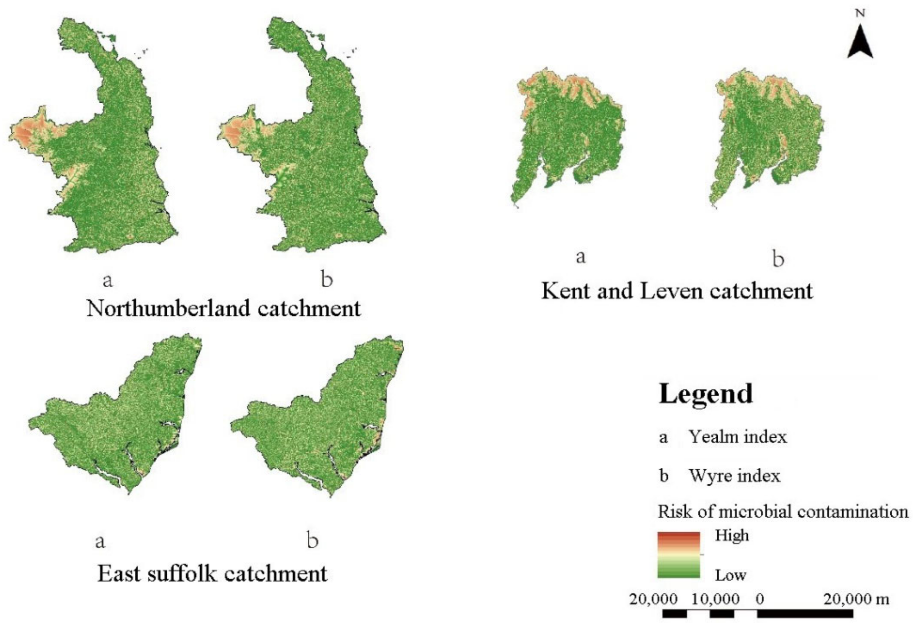
The fecal microbial risk map shows the key source area of risk—that is, the area most likely to produce microbial pollution risk—which is the upslope area weighted by the Wyre and Yealm land cover indexes (Figure 5). The color change from green to red represents the risk moving from a low to high level; ‘a’ represents the risk map corresponding to the land cover coefficient of Yealm; and ‘b’ represents the risk map corresponding to the land cover coefficient of Wyre. It can be seen that the key source areas of microbial pollution in Northumberland are distributed in the west, while the key source areas of microbial pollution in East Suffolk are distributed around the eastern edge, and the key source areas of microbial pollution in Kent and Leven are mainly distributed in the north.
3.5. The Relationship between the Land Cover Contribution Area and E. coli
A univariate linear regression analysis was carried out on the geometric mean of the E. coli concentration in the dry and wet seasons and the upslope area weighted by the Yealm and Wyre parameter groups. The result is included in Table 5. In this study, adjusted R2 was selected to measure the calibration effect of the model. The closer R2 was to 1, the better the fitting effect of the predicted risk and observed risk was. In contrast, the closer R2 was to 0, the worse the fitting effect of the predicted risk and observed risk was. Considering the significance in correlation analysis, the significance in the analysis of the East Suffolk catchment is less than 0.01 (both rainy season and dry season), and the credibility of the result is relatively high. This research believes that the available measured value data from Northumberland and Kent and Leven are so small that there may be a relatively large deviation between the actual value obtained by the researchers through geometric averaging and the real situation. This may be a reason why the p value is larger than 0.05.
4. Discussion
4.1. Assessment of Models: Prediction of Microbial Pollution and Transferability of Land Cover Parameters
Table 5 and Figure 5 show that both the Wyre and Yealm models are able to sufficiently predict and explain the microbial pollution risks and generate risk maps in the East Suffolk catchment. This also shows that land cover parameters have certain transferability.
The three catchments had different performance effects on the Wyre and Yealm parameter settings, indicating that the transfer of land cover weight has adaptive conditions and limitations. In fact, in the field of environmental pollution monitoring, there have been many examples of research studying the transferability of model parameters. For example, the model parameters of unmeasured basins can be regionalized by using the regression method or by measuring the distance between known parameter basins and unmeasured basins, which is called Prediction in Ungauged Basin (PUB). Hrachowitz et al. [31] stated that in the efforts made by PUB to regionalize the model parameters of ungauged stations, regression methods or some distance measures between gauged and ungauged sites can be used (including the spatially closest stream gauge data and the hydrological data of the gauge station most relevant to the ungauged site). The authors of [32] tested the transferability of the main parameters (within the same basin, adjacent basins, and basins under different environment settings) of a half-distributed SWAT model and found that the parameters could be reasonably transferred between adjacent basins. However, the aspect of transferability between catchments with different geographical conditions still needs to be considered. The research of these authors also showed that the performance of the model declined slightly as time and space increased. Regarding this point, Zalzal, et al. [33] also presented similar descriptions in their studies on land use regression (LUR) models. They hold the view that LUR models seem to support transferability between cities with similar geographical circumstances. Therefore, it is estimated in this paper that the parameters of the diffuse pollution monitoring model are generally transferable and applicable to study sites with adjacent geographical locations or similar geographical conditions (such as similar land cover compositions).
It can be seen from Table 3 that in the Yealm land cover parameter system, on cultivated land, improved grassland, and forest land, there was no impact (0.54), dilution (0.08), and dilution (0.19), respectively. In the Wyre parameter system, the corresponding types of impact were dilution (0.18), contribution (0.63), and dilution (0.04). When different parameter groups are used in the same model, they may obtain similar results (equivalence) [34]; this may explain why the Wyre parameter and the Yealm parameter showed similar results in East Suffolk. This may occur because the dilution and contribution of some parameters have an offset effect. For example, the contribution of improved grassland to freshwater pollution in the Wyre parameter group may have been greatly diluted by the effects of the cultivated land and forest land.
4.2. Limitation and Uncertainty
There are some possible reasons for poor levels of transferability or prediction. First, it is possible that a certain land use type does not exist in an area, or that it only represents a small portion of the whole land cover of an area (such as rough grazing), which may mean that the land use signal is weak and ineffective. Second, the availability of FIOs in the same land cover category may differ due to the use of too-wide coverage areas, affecting the outputs of the model [28]. Improved grassland coverage levels include many different management regimes that may represent different levels of availability of FIOs. For instance, for livestock grazing purposes, the source of FIOs takes the form of livestock fecal deposits, while for silage production management purposes, the risk of FIO contamination is in the form of slurry. Second, the category of improved grassland may be used to raise different kinds of livestock in different areas, and the FIO survival rate in the different feces of different livestock may also be different. The research results of Hodgson, et al. [35] showed that the E. coli survival rates were in the order of dairy cattle slurry > beef cattle farmyard manure > beef cattle feces > sheep feces. Differences in livestock density in different places may also be an important factor affecting these results. The Automated Land-based Activity Risk Assessment (ALARM) export potentials produced for various land use categories indicate that parameter values will differ for land used for different agricultural purposes. For example, the parameters of irrigated commercial agriculture, dryland commercial agriculture, and subsistence agriculture were found to be 0.300, 0.300, and 1.000, respectively [30]. This paper classified areas used for different agricultural purposes as arable land and set the parameters to be the same, which may have affected the model’s accuracy. Third, as the E. coli concentration dataset spans 10 years, the land cover may have changed a lot in some CSAs, and this could have affected the model’s results.
4.3. Ideas for Policy and Environment Management for Microbial Water Pollution
The quality of freshwater should be managed on the basis of the CSAs identified by the spatial model. According to the different land types present within CSAs, different levels of mitigation should be applied. The transfer model can help regulators choose fixed locations for monitoring stations. This study produced a combined map of the study area and CSA risk. This study suggests increasing the number of monitoring stations at the east side of the Suffolk catchment, increasing the number of monitoring stations at the west side of the Northumberland catchment, and increasing the number of monitoring stations at the west side of the Northumberland catchment. For ungauged catchments, the location of pollution sampling points and monitoring sites can be determined according to the risk map.
Generally, the largest source of fecal pollution of freshwater is animal husbandry, which corresponds to the improved grassland and rough grazing land types. The pollution in those areas is mainly caused by the direct deposition of animal waste into waterways. For areas where there is a high degree of overlap between CSAs and improved grassland and rough grazing areas, an appropriate mitigation measure is to build bridges over streams to avoid the feces of livestock directly falling into freshwater as they cross streams [36]. Riparian fencing and buffering can not only prevent livestock from being drawn into waterways, but also prevent microbes from being flushed from slopes into surface runoff. The government should encourage livestock farms to be moved away from rivers and construct wetlands as buffer zones between livestock farms and freshwater sources [37].
Government or environment agencies can instruct herdsmen and farmers to reduce or avoid grazing and irrigation tasks on poorly drained soils or CSA areas. If the grazing area happens to be within the CSA, with the consent of the herdsmen, the herdsmen can be paid for their relocation expenses and given assistance to move to a low-risk area instead. The quantity of fertilizer used should be smaller than that of the soil irrigation capacity, since fertilizer irrigation can easily lead to microbial contamination seeping into groundwater when the soil water is saturated or near saturated.
Grouping animals by age has also been shown to be an effective method for reducing specific pathogens, since young animals often shed large numbers of egg sacs, while older animals do not. Hence, calf droppings should be collected separately from those of older animals [37]. It is necessary to develop bioenergy projects to develop wastewater processors (such as the Omni processor) that use wastewater solids as fuel to convert wastewater into drinking water and electricity. The government could provide reasonable funds to those who provide sewage to encourage people to reduce the direct discharge of fecal sewage from animals. For arable and urban areas, vegetated buffer strips (VBS) can be constructed and placed along both sides of the downward slope of the farmland. The principle here is that plants can effectively slow down the flow speed of liquid; with water slowly passing through buffer filters, and pollutants being left in VBS, as they have larger particle sizes than water. A good buffer zone is usually about 10 m wide, with a slope of less than 8% and a vegetation coverage of about 90%.
5. Conclusions
This model uses simple information and data to effectively generate risk maps, demonstrating that land cover weights may be transferable between catchments This research has found that the predicted values of E. coli concentration in the East Suffolk catchment in the dry and rainy reasons weighted by Yealm and Wyre are well fitted to the corresponding measured values and show good significance. Although the linear regression between the predicted value and the measured value of the Northumberland catchment and the Kent and Leven catchment cannot pass the significance test, this research maintains that the available measured value data from these two catchments are so small that there may be a relatively large deviation between the actual value obtained by the researchers through geometric averaging and the real situation. If there are more measured data, the results of error analysis are likely to be better. This research believes that increasing monitoring and providing more E. coli data by the UK’s government agencies and social organizations are not only conducive to people better understanding the microbial contamination in watersheds, but also facilitate the researchers to carry out transferability studies and explore the extent to which E. coli concentrations and microbial risks in other watersheds can be predicted through transferability. Our results can act as a guide for the construction of microbial risk models for ungauged catchments. However, this model had some limitations. First, different land use patterns may have been used for the same land cover type. Second, the impact of time span was not considered. Third, there may have been errors in the identification of land types by satellites, which may have affected the accuracy of the model. In future studies, the accuracy of the model can be improved by dividing the location of the sampling points during the monsoon and non-monsoon periods. In addition, consideration will be given to further determining the division of land types in conjunction with field visits and adding factors such as fecal density into the model. In terms of mitigating microbial contamination, the identified key risk sources should be divided across different types of land cover and managed in a targeted manner. Livestock manure management should be carried out in improved grasslands and rough grazing areas, and vegetation buffer zones should be used to alleviate manure pollution in arable areas.
Author Contributions
Conceptualization, J.L. (Jiawei Li) and J.L. (Junyou Liu); Data curation, J.L. (Jiawei Li) and J.L. (Junyou Liu); Methodology, J.L. (Jiawei Li); Supervision, J.L. (Junyou Liu); Writing—original draft, J.L. (Jiawei Li); Writing—review and editing, J.L. (Junyou Liu). All authors have read and agreed to the published version of the manuscript.
Funding
This research received no external funding.
Institutional Review Board Statement
Not applicable.
Informed Consent Statement
Not applicable.
Data Availability Statement
Not applicable.
Acknowledgments
I am Jiawei Li. As the first author of this article, I feel very grateful to my supervisor Jim Wright, who is in GIS and International Development at the University of Southampton. He helped me a great deal in determining my research direction and guiding me in carrying out this research. I would like to say that if this article is successfully published, it would not have been possible without the guidance and supervisory support of Jim Wright.
Conflicts of Interest
The authors declare no conflict of interest.
References
- Sarker, S.; Veremyev, A.; Boginski, V.; Singh, A. Critical Nodes in River Networks. Sci. Rep. 2019, 9, 11178. [Google Scholar] [CrossRef] [PubMed] [Green Version]
- Sarker, S. Investigating Topologic and Geometric Properties of Synthetic and Natural River Networks under Changing Climate; University of Central Florida: Orlando, FL, USA, 2021. [Google Scholar]
- Pandey, P.K.; Kass, P.H.; Soupir, M.L.; Biswas, S.; Singh, V.P. Contamination of water resources by pathogenic bacteria. AMB Express 2014, 4, 16. [Google Scholar] [CrossRef] [PubMed] [Green Version]
- Price, R.; Wildeboer, D. Escherichia coli—Recent Advances on Physiology, Pathogenesis and Biotechnological Applications; IntechOpen: Rijeka, Croatia, 2017. [Google Scholar]
- Jamieson, R.; Gordon, R.; Joy, D.; Lee, H. Assessing microbial pollution of rural surface waters—A review of current watershed scale modeling approaches. Agric. Water Manag. 2004, 70, 1–17. [Google Scholar] [CrossRef]
- Kay, D.; Crowther, J.; Stapleton, C.M.; Wyer, M.D. Faecal indicator organism inputs to watercourses from streamside pastures grazed by cattle: Before and after implementation of streambank fencing. Water Res. 2018, 143, 229–239. [Google Scholar] [CrossRef] [PubMed] [Green Version]
- Rajan, R.J.; Sudarsan, J.S.; Nithiyanantham, S. Efficiency of constructed wetlands in treating E. coli bacteria present in livestock wastewater. Int. J. Environ. Sci. Technol. 2020, 17, 2153–2162. [Google Scholar] [CrossRef]
- Bu, C.H.; Lai, S.H.; Goh, X.T.; Chong, W.T.; Chin, R.J. Influence of filter media depth and vegetation on Faecal Coliform removal by stormwater biofilters. Water Environ. J. 2021, 35, 181–189. [Google Scholar] [CrossRef]
- Lane, S.N.; Brookes, C.J.; Heathwaite, A.L.; Reaney, S. Surveillant science: Challenges for the management of rural environments emerging from the new generation diffuse pollution models. J. Agric. Econ. 2006, 57, 239–257. [Google Scholar] [CrossRef]
- Milledge, D.G.; Lane, S.N.; Heathwaite, A.L.; Reaney, S.M. A Monte Carlo approach to the inverse problem of diffuse pollution risk in agricultural catchments. Sci. Total Environ. 2012, 433, 434–449. [Google Scholar] [CrossRef] [Green Version]
- Parajuli, P.B.; Mankin, K.R.; Barnes, P.L. Applicability of targeting vegetative filter strips to abate fecal bacteria and sediment yield using SWAT. Agric. Water Manag. 2008, 95, 1189–1200. [Google Scholar] [CrossRef]
- Pease, L.M.; Oduor, P.; Padmanabhan, G. Estimating sediment, nitrogen, and phosphorous loads from the Pipestem Creek watershed, North Dakota, using AnnAGNPS. Comput. Geosci. 2010, 36, 282–291. [Google Scholar] [CrossRef]
- Ribarova, I.; Ninov, P.; Cooper, D. Modeling nutrient pollution during a first flood event using HSPF software: Iskar River case study, Bulgaria. Ecol. Model. 2008, 211, 241–246. [Google Scholar] [CrossRef]
- Matthews, R. The People and Landscape Model (PALM): Towards full integration of human decision-making and biophysical simulation models. Ecol. Model. 2006, 194, 329–343. [Google Scholar] [CrossRef]
- Ekholm, P.; Turtola, E.; Gronroos, J.; Seuri, P.; Ylivainio, K. Phosphorus loss from different farming systems estimated from soil surface phosphorus balance. Agric. Ecosyst. Environ. 2005, 110, 266–278. [Google Scholar] [CrossRef]
- Haag, D.; Kaupenjohann, M. Landscape fate of nitrate fluxes and emissions in Central Europe—A critical review of concepts, data, and models for transport and retention. Agric. Ecosyst. Environ. 2001, 86, 1–21. [Google Scholar] [CrossRef]
- Wolf, J.; Hack-ten Broeke, M.J.D.; Rotter, R. Simulation of nitrogen leaching in sandy soils in The Netherlands with the ANIMO model and the integrated modelling system STONE. Agric. Ecosyst. Environ. 2005, 105, 523–540. [Google Scholar] [CrossRef]
- Lam, Q.D.; Schmalz, B.; Fohrer, N. Modelling point and diffuse source pollution of nitrate in a rural lowland catchment using the SWAT model. Agric. Water Manag. 2010, 97, 317–325. [Google Scholar] [CrossRef]
- Li, Z.F.; Luo, C.; Xi, Q.; Li, H.P.; Pan, J.J.; Zhou, Q.S.; Xiong, Z.Q. Assessment of the AnnAGNPS model in simulating runoff and nutrients in a typical small watershed in the Taihu Lake basin, China. Catena 2015, 133, 349–361. [Google Scholar] [CrossRef]
- Mishra, A.; Kar, S.; Singh, V.P. Determination of runoff and sediment yield from a small watershed in sub-humid subtropics using the HSPF model. Hydrol. Process. 2007, 21, 3035–3045. [Google Scholar] [CrossRef]
- Environment Agency. Download Open Water Quality Archive Datasets. Available online: https://environment.data.gov.uk/water-quality/view/download/new (accessed on 4 April 2020).
- Digimap. OS Data Download. Available online: https://digimap.edina.ac.uk/roam/download/os (accessed on 1 June 2020).
- Xu, F.; Dong, G.X.; Wang, Q.R.; Liu, L.M.; Yu, W.W.; Men, C.; Liu, R.M. Impacts of DEM uncertainties on critical source areas identification for non-point source pollution control based on SWAT model. J. Hydrol. 2016, 540, 355–367. [Google Scholar] [CrossRef]
- Land Cover Map. Available online: https://digimap.edina.ac.uk/roam/download/environment (accessed on 3 June 2020).
- Porter, K.D.H.; Reaney, S.M.; Quilliam, R.S.; Burgess, C.; Oliver, D.M. Predicting diffuse microbial pollution risk across catchments: The performance of SCIMAP and recommendations for future development. Sci. Total Environ. 2017, 609, 456–465. [Google Scholar] [CrossRef]
- Lane, S.N.; Reaney, S.M.; Heathwaite, A.L. Representation of landscape hydrological connectivity using a topographically driven surface flow index. Water Resour. Res. 2009, 45, 10. [Google Scholar] [CrossRef] [Green Version]
- Heathwaite, A.L.; Quinn, P.F.; Hewett, C.J.M. Modelling and managing critical source areas of diffuse pollution from agricultural land using flow connectivity simulation. J. Hydrol. 2005, 304, 446–461. [Google Scholar] [CrossRef]
- Vogel, R.M. The geometric mean? Commun. Stat. Theory Methods 2022, 51, 82–94. [Google Scholar] [CrossRef]
- Chen, J. Basics of Statistics; Beijing Institute of Technology Press: Beijing, China, 2013. [Google Scholar]
- Rozovsky, L.V. Comparison of Arithmetic, Geometric, and Harmonic Means. Math. Notes 2021, 110, 118–125. [Google Scholar] [CrossRef]
- Hrachowitz, M.; Savenije, H.H.G.; Bloschl, G.; McDonnell, J.J.; Sivapalan, M.; Pomeroy, J.W.; Arheimer, B.; Blume, T.; Clark, M.P.; Ehret, U.; et al. A decade of Predictions in Ungauged Basins (PUB)—A review. Hydrol. Sci. J.-J. Sci. Hydrol. 2013, 58, 1198–1255. [Google Scholar] [CrossRef]
- Heuvelmans, G.; Muys, B.; Feyen, J. Evaluation of hydrological model parameter transferability for simulating the impact of land use on catchment hydrology. Phys. Chem. Earth Parts A/B/C 2004, 29, 739–747. [Google Scholar] [CrossRef]
- Zalzal, J.; Alameddine, I.; El Khoury, C.; Minet, L.; Shekarrizfard, M.; Weichenthal, S.; Hatzopoulou, M. Assessing the transferability of landuse regression models for ultrafine particles across two Canadian cities. Sci. Total Environ. 2019, 662, 722–734. [Google Scholar] [CrossRef]
- Beven, K. Prophecy, reality and uncertainty in distributed hydrological modelling. Adv. Water Resour. 1993, 16, 41–51. [Google Scholar] [CrossRef]
- Hodgson, C.J.; Bulmer, N.; Chadwick, D.R.; Oliver, D.M.; Heathwaite, A.L.; Fish, R.D.; Winter, M. Establishing relative release kinetics of faecal indicator organisms from different faecal matrices. Lett. Appl. Microbiol. 2009, 49, 124–130. [Google Scholar] [CrossRef] [Green Version]
- Collins, R.; McLeod, M.; Hedley, M.; Donnison, A.; Close, M.; Hanly, J.; Horne, D.; Ross, C.; Davies-Colley, R.; Bagshaw, C.; et al. Best management practices to mitigate faecal contamination by livestock of New Zealand waters. N. Z. J. Agric. Res. 2007, 50, 267–278. [Google Scholar] [CrossRef]
- Hutchison, M.L.; Walters, L.D.; Avery, S.M.; Munro, F.; Moore, A. Analyses of livestock production, waste storage, and pathogen levels and prevalences in farm manures. Appl. Environ. Microbiol. 2005, 71, 1231–1236. [Google Scholar] [CrossRef] [PubMed]
Figure 1.
Map of the study area.
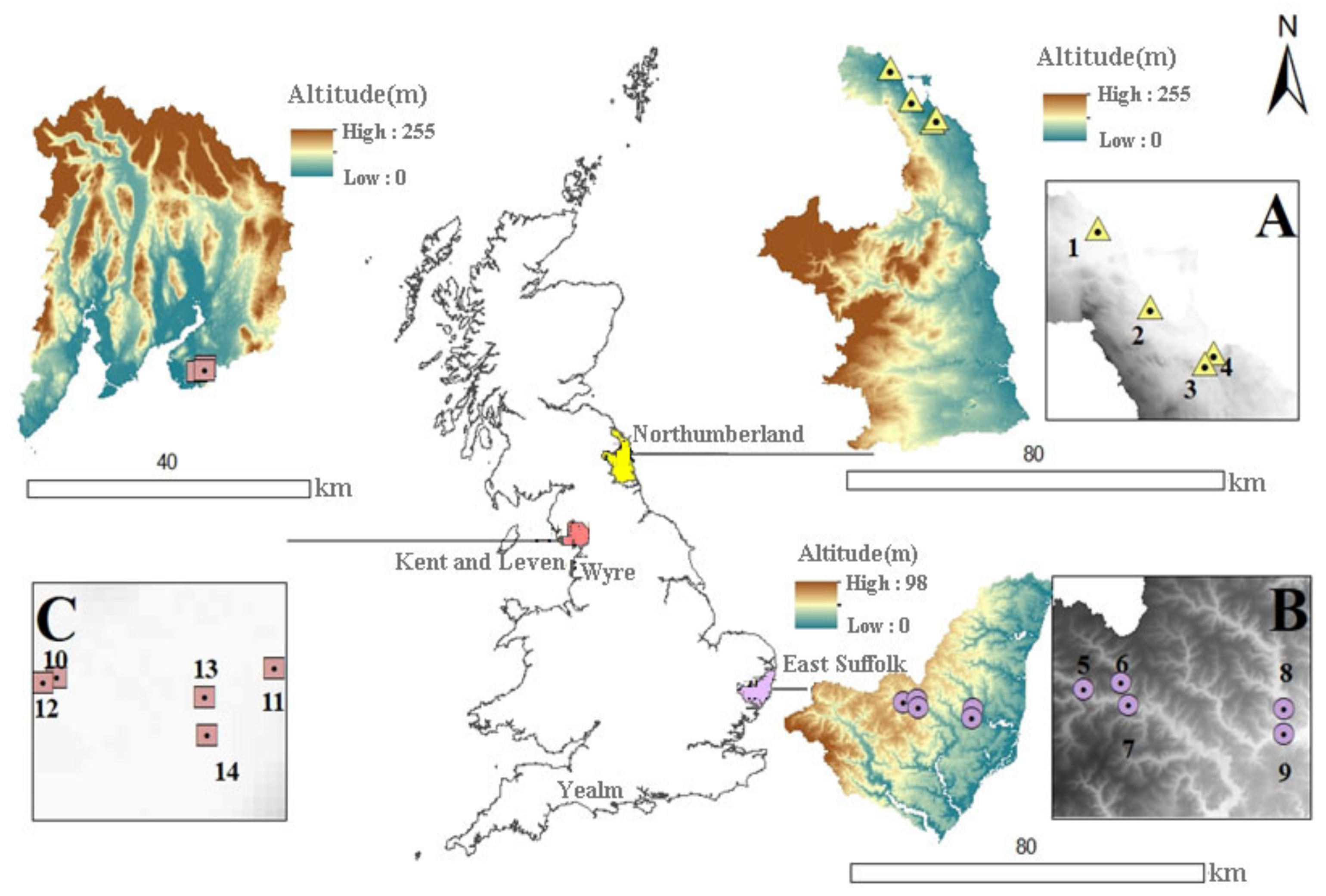
Figure 2.
A bar chart shows the proportion of different land cover types among the study sites [25].
Figure 2.
A bar chart shows the proportion of different land cover types among the study sites [25].

Figure 3.
The geometric E. coli concentration variation among the study sites.
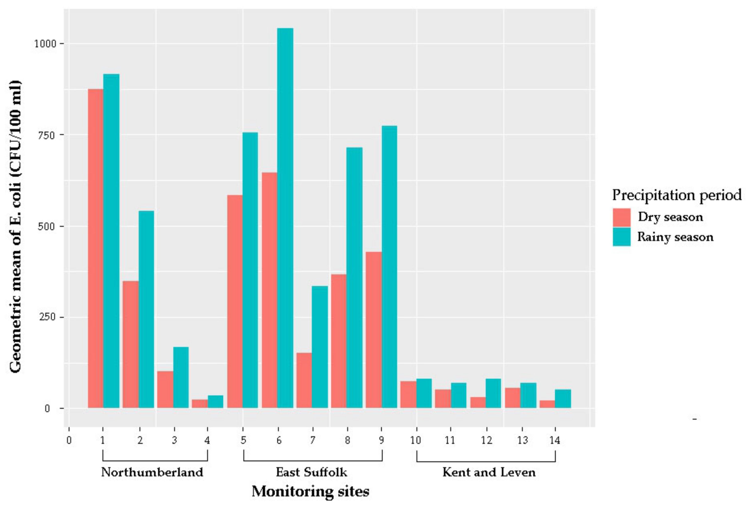
Figure 4.
The change in the area of upslope accumulation weighted by different parameters at different monitoring points.
Figure 4.
The change in the area of upslope accumulation weighted by different parameters at different monitoring points.
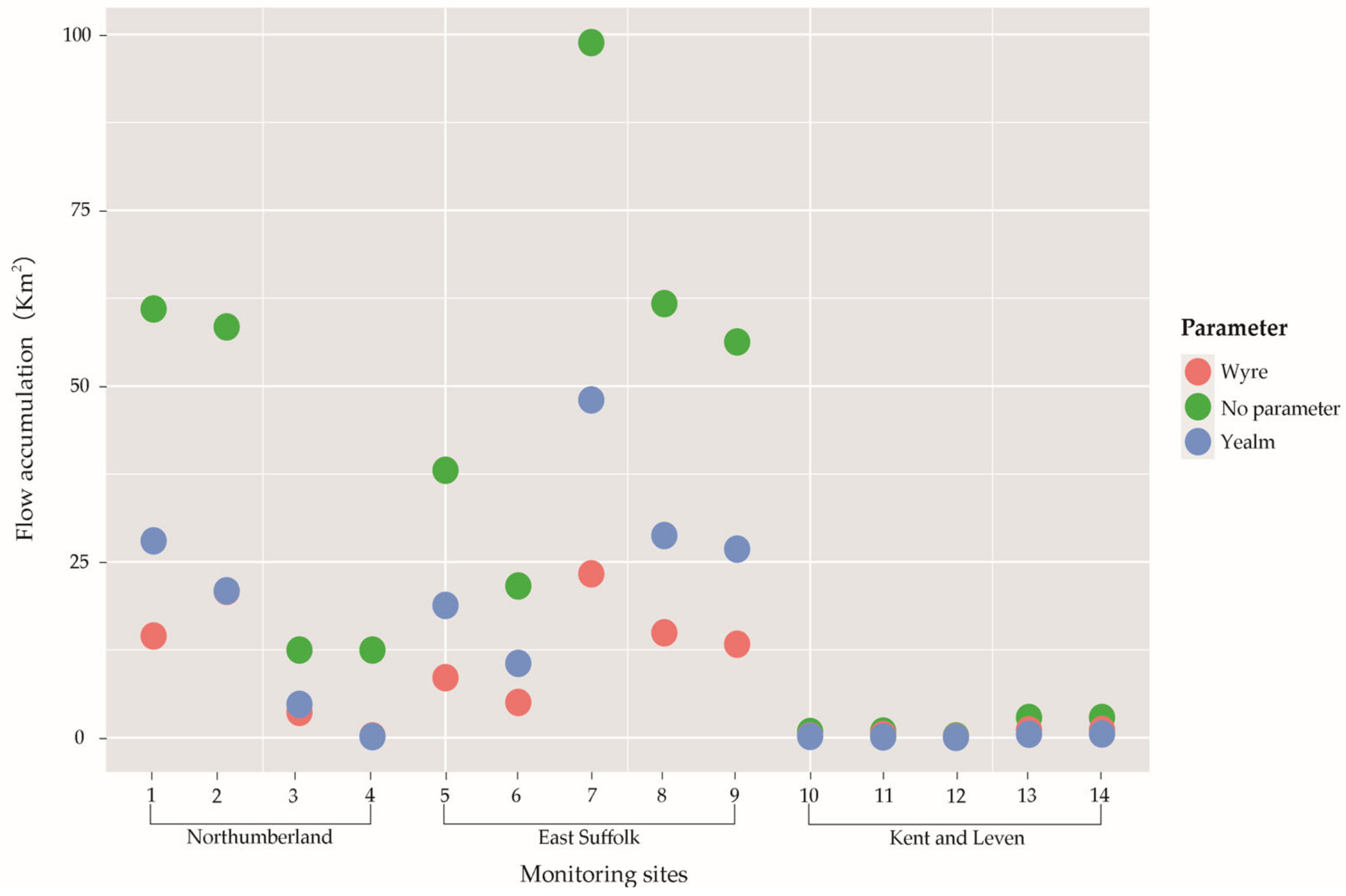
Figure 5.
CSA risk map of fecal microbial contamination.

Table 1.
Comparison of the different modeling approaches used to identify non-point pollution in catchments [14,15,16,17,18,19,20].
| Model Type | Explanation | Characteristics | Water Quality Parameters | Spatial Unit | Classification of Land Cover Type | Software | Author |
|---|---|---|---|---|---|---|---|
| Transfer function modelling (export coefficient modelling approach) | Based on transfer function, obtain the output with known inputs, such as fertilizers and manure | The calculation method is simple, but the accuracy is not high | Phosphorus (kg ha−1 year−1) | / | / | / | Ekholm et al. [14] |
| Nitrate (kg ha−1 year−1) | Haag [15] | ||||||
| Land unit modelling | Predict the concentration of pollutants in freshwater based on individual land units, such as grid square, regardless of spatial heterogeneity | The relative accuracy of the results is high, but it is not possible to investigate areas lacking data | Carbon and nitrogen (kg ha−1 year−1) | / | Crops, food, livestock | The People and Landscape Model (PALM) | Matthews [16] |
| Nitrate (kg ha−1 year−1) | 250 m × 250 m | Grassland, beets, maize | ANIMO model and STONE | Wolf et al. [17] | |||
| Land transfer modelling | On the basis of land unit modelling, cross-landscape dynamic analysis is carried out | The process of pollution generation and transfer is simulated based on the concept of connectivity; this has a higher accuracy | Nitrate (kg ha−1 year−1) | 25 m × 25 m | Agricultural land, deciduous forest land, evergreen forest land, pasture land, range brush land, range grass land, urban land, and water | SWAT model | Lam et al. [18] |
| Nitrogen and phosphorus (kg ha−1 year−1) | 30 m × 30 m | Bare land, urban land, agricultural land, forest, grassland, water body | AnnAGNPS model | Li et al. [19] | |||
| Sediment (t/ha) | 30 m × 30 m | Deep water, shallow water, dense forest, growing forest, paddy, upland crops, fallow land, and eroded land | HSPF | Mishra et al. [20] |
Table 2.
Centre for Ecology and Hydrology Land Cover Map classes for 2015 and how they are condensed for reclassification.
Table 2.
Centre for Ecology and Hydrology Land Cover Map classes for 2015 and how they are condensed for reclassification.
| CEH Class | Description | SCIMAP Class |
|---|---|---|
| Broadleaved woodland and coniferous woodland | Deciduous, mixed, conifer, larch, evergreen, felled forest, scrub and new plantation | Woodland |
| Arable and horticulture | Arable bare ground, freshly ploughed land, cereal, non-cereal, horticulture, and rational horticulture | Arable |
| Improved grassland | Intensively managed grassland for hay, silage, and grazing marsh | Improved grassland |
| Neutral grassland, calcareous grassland, acid grassland | Semi-natural grassland and managed low-productivity grassland | Rough grazing |
| Fen, marsh, swamp, bog, saltmarsh | Swamp, fen/marsh, fen willow, bog, shrub, grass/shrub and undifferentiated (all on deep peat) | Bog |
| Heather, heather grassland | Heather grassland and exposed rock as well as habitats occurring at higher altitudes | Moorland |
| Inland rock, saltwater, freshwater, supra-littoral rock, supra-littoral sediment, littoral rock, littoral sediment | Coastal water, rivers, canals, and standing water; coastal rock and sediment | Other |
| Urban, suburban | Urban areas, including towns, cities, docksides, industrial estates, and car parks; suburban areas including a mix of built-up areas and vegetation | Urban |
Table 3.
The optimum combination of land cover parameters in Wyre and Yealm and the role they play in the operation of the model (dilution or diffusion). Modified from [25].
Table 3.
The optimum combination of land cover parameters in Wyre and Yealm and the role they play in the operation of the model (dilution or diffusion). Modified from [25].
| Land Cover Type/Position Name | Yealm | Diffuse or Dilute to FIO Pollution | Wyre | Contribute or Dilute to FIO Pollution |
|---|---|---|---|---|
| Improved grassland | 0.08 | High dilution | 0.63 | Medium diffusion |
| Rough grazing | 0.78 | High diffusion | 0.58 | Medium diffusion |
| Moorland | 0.5 | Not influential | 0.52 | Not influential |
| Bog | 0.5 | Not influential | 0.49 | Not influential |
| Urban | 0.5 | Not influential | 0.52 | Not influential |
| Arable | 0.54 | Not influential | 0.18 | High dilution |
| Woodland | 0.19 | High dilution | 0.04 | High dilution |
Table 4.
The upslope area weighted by different parameters varies among the different study sites.
| Monitoring Points | Catchments | Unweighted Flow Accumulation (Km2) | Wyre Weighted Flow Accumulation (Km2) | Yealm Weighted Flow Accumulation (Km2) |
|---|---|---|---|---|
| 1 | Northumberland | 60.98925 | 14.47405 | 28.0045 |
| 2 | Northumberland | 58.41975 | 20.8057 | 20.90293 |
| 3 | Northumberland | 12.49323 | 3.6116 | 4.73415 |
| 4 | Northumberland | 12.49323 | 0.235556 | 0.14814 |
| 5 | East Suffolk | 38.04375 | 8.542375 | 18.83795 |
| 6 | East Suffolk | 21.59735 | 5.002875 | 10.57358 |
| 7 | East Suffolk | 98.862 | 23.30825 | 48.0325 |
| 8 | East Suffolk | 61.724 | 14.92693 | 28.75775 |
| 9 | East Suffolk | 56.26825 | 13.31958 | 26.84325 |
| 10 | Kent and Leven | 0.857025 | 0.27527 | 0.182128 |
| 11 | Kent and Leven | 0.9558 | 0.4811 | 0.112465 |
| 12 | Kent and Leven | 0.282175 | 0.137879 | 0.074914 |
| 13 | Kent and Leven | 2.881125 | 1.13017 | 0.501063 |
| 14 | Kent and Leven | 2.904175 | 1.140095 | 0.511477 |
Table 5.
Prediction of the regression models between geometric mean FIO (E. coli) concentrations and rainfall accumulation areas weighted by different parameters.
Table 5.
Prediction of the regression models between geometric mean FIO (E. coli) concentrations and rainfall accumulation areas weighted by different parameters.
| Dependent Variable | Independent Variable | Adjusted R2 | Significance |
|---|---|---|---|
| Objective Risk | Predicted Risk | ||
| Geometric average of the E. coli concentration in the Northumberland catchment during the wet season | Northumberland upslope area weighted by the Yealm land cover weight | 0.955 | p < 0.05 |
| Northumberland upslope area weighted by the Wyre land cover weight | 0.42 | p > 0.05 | |
| Geometric average of the E. coli concentration in the Northumberland catchment during the dry season | Northumberland upslope area weighted by the Yealm land cover weight | 0.799 | p > 0.05 |
| Northumberland upslope area weighted by the Wyre land cover weight | 0.124 | p > 0.05 | |
| Geometric average of the E. coli concentration in the East Suffolk catchment during the wet season | East Suffolk upslope area weighted by the Yealm land cover weight | 0.916 | p < 0.01 |
| East Suffolk upslope area weighted by the Wyre land cover weight | 0.872 | p < 0.01 | |
| Geometric average of the E. coli concentration in the East Suffolk catchment during the dry season | East Suffolk upslope area weighted by the Yealm land cover weight | 0.969 | p < 0.01 |
| East Suffolk upslope area weighted by the Wyre land cover weight | 0.991 | p < 0.01 | |
| Geometric average of the E. coli concentration in the Kent and Leven catchment during the wet season | Kent and Leven upslope area weighted by the Yealm land cover weight | 0.545 | p > 0.05 |
| Kent and Leven upslope area weighted by the Wyre land cover weight | 0.644 | p > 0.05 | |
| Geometric average of the E. coli concentration in the Kent and Leven catchment during the dry season | Kent and Leven upslope area weighted by the Yealm land cover weight | −0.162 | p > 0.05 |
| Kent and Leven upslope area weighted by the Wyre land cover weight | −0.173 | p > 0.05 |
Publisher’s Note: MDPI stays neutral with regard to jurisdictional claims in published maps and institutional affiliations. |
© 2022 by the authors. Licensee MDPI, Basel, Switzerland. This article is an open access article distributed under the terms and conditions of the Creative Commons Attribution (CC BY) license (https://creativecommons.org/licenses/by/4.0/).
Share and Cite
MDPI and ACS Style
Li, J.; Liu, J. Predicting Freshwater Microbial Pollution Using a Spatial Model: Transferability between Catchments. Sustainability 2022, 14, 13583. https://doi.org/10.3390/su142013583
AMA Style
Li J, Liu J. Predicting Freshwater Microbial Pollution Using a Spatial Model: Transferability between Catchments. Sustainability. 2022; 14(20):13583. https://doi.org/10.3390/su142013583
Chicago/Turabian StyleLi, Jiawei, and Junyou Liu. 2022. "Predicting Freshwater Microbial Pollution Using a Spatial Model: Transferability between Catchments" Sustainability 14, no. 20: 13583. https://doi.org/10.3390/su142013583
Note that from the first issue of 2016, this journal uses article numbers instead of page numbers. See further details here.