

Network-Based Space-Time Scan Statistics for Detecting Micro-Scale Hotspots
1
Department of Geography, Birkbeck, University of London, London WC1E 7HX, UK
2
Department of Geography, Geology and the Environment, Kingston University, Kingston upon Thames KT1 2EE, UK
*
Author to whom correspondence should be addressed.
Sustainability 2022, 14(24), 16902; https://doi.org/10.3390/su142416902
Submission received: 15 October 2022
/
Revised: 26 November 2022
/
Accepted: 13 December 2022
/
Published: 16 December 2022
(This article belongs to the Special Issue The New Science of Cities and Urban Growth Sustainability)
Abstract
:Events recorded in urban areas are often confined by the micro-scale geography of street networks, yet existing spatial–analytical methods do not usually account for the shortest-path distance of street networks. We propose space–time NetScan, a new spatial–temporal analytical method with improved accuracy for detecting patterns of concentrations across space and time. It extends the notion of a scan-statistic-type search window by measuring space-time patterns along street networks in order to detect micro-scale concentrations of events at the street-address level with high accuracy. Performance tests with synthetic data demonstrate that space-time NetScan outperforms existing methods in detecting the location, shape, size and duration of hotspots. An empirical study with drug-related incidents shows how space-time NetScan can improve our understanding of the micro-scale geography of crime. Aside from some abrupt one-off incidents, many hotspots form recurrent hotbeds, implying that drug-related crimes tend to persist in specific problem places.
1. Introduction
Detection of spatial and spatial–temporal concentrations of events marks one of the pillars across many disciplines that investigate problem places and times. In the field of geography, its foundations were laid as early as in the 1960s, in part as an integral component of a paradigm shift known as the quantitative revolution (Chorley and Haggett, 1967 [1]). Since that time, spatial and spatial–temporal cluster analyses have been pursued in a number of fields, including forestry, ecology, epidemiology and urban geography, primarily in the forms of cluster detection and hotspot analysis (Clark and Evans, 1954 [2]; Diggle et al., 1976 [3]; Ripley, 1976 [4]; Ripley, 1981 [5]; Boots and Getis, 1988 [6]; Knox, 1989 [7]; Kulldorff and Nagarwalla, 1995 [8]; Rogerson 2001 [9]).
In the context of geography of crime, the detection of problem places has been studied rigorously, especially in the last two decades (Weisburd et al., 2004 [10]; Braga et al., 2010 [11]; Weisburd and Telep, 2014 [12]; Lee et al., 2017 [13]; Oliveira and Bastos-Filho, 2017 [14]; Mohler et al., 2020 [15]). In particular, small, concentrated areas of high risk, namely micro-scale crime hotspots, have attracted strong attention, as they show places where crime problems are most active at the scale that relates closely to the recent crime-and-place studies and policing tactics (Weisburd, 2015 [16]; O’brien and Winship, 2017 [17]. However, the existing range of methods for identifying crime hotspots, either spatially or across space and time, are not always suitable for detecting hotspots at the micro scale. This paper proposes a new type of method for detecting micro-scale space-time crime hotspots; a method that employs the scale unit of micro-scale universe in its analysis, designed to provide a more accurate description of the spatial–temporal patterns of crime incidents. Through its application in the analysis of drug-related crimes, we aim to demonstrate the effectiveness of the proposed method to improve our understanding of the micro-scale geography of crime.
2. Related Work
Much of the literature on crime-and-place studies have investigated the patterns of crimes aggregated to areal units (Robinson, 1982 [18]; Evans and Herbert, 1989 [19]; Weisburd and McEwan, 1998 [20]). While areal data offer valuable insights into the association between the crime level and the characteristics attached to each area, they do not offer robust narratives on how and why crime incidents concentrate on specific problem places. Recent criminological theory has stressed that crime opportunities at specific micro places hold a key to unravelling the mechanism of crime occurrences (Braga and Weisburd, 2010 [21]; Braga et al., 2014 [22]; Weisburd and Telep, 2014 [12]). For instance, Weisburd et al. (2012) [23] examined the spatial extent of crime opportunities using a vast amount of micro-scale level data on guardians, accessibility and crime targets, confirming the presence of micro-scale crime opportunities using street segments as the unit of measurement. Findings from these studies suggest that detailed crime opportunities can be clarified only by detecting and understanding crime hotspots at the micro scale, rather than following the change in the patterns of crime at the aggregate level.
The importance of identifying micro-scale crime hotspots is also recognised for practical and professional policing purposes—a number of crime prevention schemes established recently by law enforcement agencies focus on crime hotspots (i.e., hotspot policing) (Braga, 2001 [24]; Weisburd and Eck, 2004 [25]; Weisburd and Braga, 2006 [26]; Weisburd et al., 2009 [27]; Dau et al., 2022 [28]). The fact that a large portion of crime is concentrated in small and specific places on the street makes hotspot policing particularly effective for reducing overall crime and disorder (Braga et al., 2019 [29]). For instance, Braga et al. in 2008 [30] reported that in 2006, over 50% of gun crimes recorded in a neighbourhood of Boston took place in 5% of the study area. At the city-wide scale, 74% of serious gun assault incidents were found within 5% of all streets of Boston (Braga et al., 2010 [11]). Similarly, Weisburd and Zastrow (2021) [31] discovered that about 1% of streets in NYC hosted about 25% of crimes recorded across the city. Investigating this tendency even further, Lee et al. 2017 [13] reported that crime is more concentrated at an address level than other units, including street segments.
Investigation of hotspots on the micro scale is also affected by the configuration of the street network; that is, streets become an important place for measuring crime, as it confines the movement of people—including motivated offenders, potential targets and passers-by (Eck 1995 [32]). Indeed, a number of studies in environmental criminology suggest that street networks play a key role in practical crime prevention as well as in exploring crime aetiology (Eck and Weisburd, 1995 [33]; Sherman, 1995 [34]; Taylor, 1997 [35]; Taylor, 1998 [36]; van Wilsem, 2009 [37]; di Bella et al. 2017, [38]). Brantingham and Brantingham (1999) [39] offered a theoretical underpinning to explicitly discuss the importance of street networks in understanding crime problems. They point out that the structures of street networks—represented by nodes and edges—along with the patterns of traffic and transits, strongly affect the distribution of crime incidents. Nevertheless, only a limited number of studies on the geography of crime incorporate the metrics and dimensions of street networks in their micro-scale analysis.
One of these efforts was made by Bowers and Johnson (2005) [40], who reported that properties within 400 m in street distance of a burgled home are subject to an elevated risk of crime for up to two months after the initial incident, with properties on the same side of the street as the burgled home being subjected to a higher risk. They focus on crime forecasting and try to predict when the next crime is likely to happen following a previous incident. While this is an important inquiry, it predicts a more global tendency that applies to the entire study area and is therefore different from detecting hotspots at a specific place. Another study was pursued by Okabe and Satoh (2009) [41], who applied a network-based k-function method to detect hotspots among burglary data in Kyoto. While their analysis was carried out in the network dimension, their study confirms a global tendency of the presence of crime concentration, rather than detecting specific micro places where such concentrations exist.
The other element that affects the patterns of crime concentration is the distribution of crime across time (Newton and Felson, 2015) [42]. A series of evidence-based criminological studies have confirmed the tendency of crime incidents to exhibit concentrations in both space and time (Braga et al., 2010 [11]; Braga et al., 2011 [43]; Groff et al., 2010 [44]; Weisburd et al., 2012 [23]; Levine et al., 2017 [45]). For instance, Weisburd et al. in 2012 [23] confirmed the generally stable and persistent nature of crime hotspots, reporting that 23% of the crimes in a city during the study period were found in chronic crime hotspots occupying less than 1% of the street segments. This suggests that a comprehensive understanding of crime hotspots in a micro setting requires simultaneous investigation of the spatial as well as the temporal patterns of crime. Other studies point out the importance of planning the practical policing strategies with respect to the spatial–temporal patterns of crime and that focusing policing resources on spatially and temporally confined hotspots would improve the effectiveness of policing intervention (Johnson et al., 2007 [46], Johnson et al., 2008 [47]; Weisburd, 2015 [16]). Some recent studies have extended spatial analytical methods to detect and evaluate space-time hotspots, but their measurements are not based on the distance along the street networks (Brunsdon et al., 2007 [48]; Neill and Gorr, 2007 [49], Nakaya and Yano, 2010 [50], Malleson and Anderson, 2015 [51]). Network-based analysis has recently seen a rise in its methodological development, especially in the broader area of spatial analysis (Okabe and Sugihara, 2012 [52]). These include studies by Okabe, Satoh and Sugihara (2009) [53], who presented kernel density estimation defined on a street network. Additionally, Yamada and Thill (2010) [54] and Nie et al. (2015) [55] extended local spatial autocorrelation methods to the network space. However, most of them have yet to incorporate the temporal patterns in their analysis. In the domain of crime forecasting, Rosser et al. in 2017 [56] took a modelling approach to predicting crime occurrences in the network space. They compared the prediction performance of their network-based model with its grid-based counterpart and concluded that the network-based model outperformed the grid-based approach on prediction accuracy. Their findings offer a strong support for the use of street level data and network-based methods for analysing crime incidents in a micro space. When it comes to the intersection of network-based, space-time analysis and micro-scale crime hotspot detection, only a handful of studies have emerged so far. In particular, Shiode and Shiode (2013) [57] and Shiode et al. (2015) [58] worked on the detection of micro-scale space-time hotspots along the street network. However, the former study (Shiode and Shiode, 2013 [57]) suffered from the use of the Bonferroni procedure (Bonferroni, 1935 [59]) in the hypothesis test, as it is known to be too conservative in detecting hotspots. Additionally, their method was designed to accommodate only a finite number of discrete searches for hotspots over space and time. The latter (Shiode et al., 2015 [58]) suggested a method using a false discovery rate (FDR) controlling procedure (Benjamini and Hochberg, 1995 [60]) in hypothesis testing for detecting hotspots, which overcomes the conservative nature of the Bonferroni-type procedures, but is still limited in its capacity to search hotspots continuously across space and time. Against this background, we propose a new type of geo-analytical method for detecting crime hotspots that overcome the major limitations, including the use of fixed-size search windows and the multiple testing problem.
3. Methodology
The methods developed in this paper expand on the notion of search windows, building partly on the framework of scan statistics—a family of hotspot detection methods that was originally proposed for epidemiological investigations (Kulldorff and Nagarwalla, 1995 [8]). Using a test statistic called a likelihood ratio test statistic (a scan statistic), they detect spatial (or space-time) zones, where event counts are significantly higher than expected. Scan statistics build on several pivotal search-window-type methods and overcome major limitations their predecessors have suffered from, including the use of fixed-size search windows and the multiple testing problem (Kulldorff and Nagarwalla, 1995 [8]; Kulldorff, 1997 [61]). For this reason, scan statistics are currently the most widely used methods of their kind, including in the geography of crime (Neill and Gorr, 2007 [49]; Cheng and Adepeju, 2014 [62]; Malleson and Andresen, 2015 [51]). While it is possible to apply scan statistics to disaggregate point data, they are designed primarily for analysing patterns across wider areal units, and their extension to network-based analysis is yet to be pursued systematically (Braga and Weisburd, 2010 [21]; Weisburd et al., 2012 [23]; Shiode and Shiode, 2013 [57]; Braga et al., 2014 [22]). The following sections explain and extend the notion of a likelihood ratio test to investigate the geographical patterns captured by search windows along a street network.
3.1. Building Scan Statistics for Searching in a Network Space
The original scan statistic (Kulldorff and Nagarwalla, 1995 [8]) uses circular search windows to identify concentrations of statistical significance. In its standard form, their search windows are produced around the centroid of predetermined aggregated areal units with their radius changing continuously from zero to a predefined upper threshold. The extent captured by each search window is considered as a potential cluster of an increased risk, and the likelihood ratio of finding the observed number of incidents is calculated by comparing the observed and the expected number of incidents inside and outside the respective window. The extent of a search window with a statistically significant underlying event-occurrence rate marks clusters, with the one that returned the highest likelihood ratio being the most likely cluster.
In this paper, the notion of the scan statistics is extended to analyse the concentration of events in or along a finite network (hereafter referred to as NetScan), whereby the standard circular search windows are replaced with network-based search windows, or search windows defined in the network space to extend along the street network. A network-based search window is constructed by identifying a point of origin (i.e., one of the reference points that are placed at a near-constant interval across the network), and extending the search window along all possible paths from that point using the Dijkstra’s shortest-path distance search until the total length of all line segments reach a pre-defined upper threshold value. Network-based search windows can cover any spatial extent within the study area and any temporal duration within the study period to identify space-time hotspots; i.e., concentration of events over space and time. The size of these search windows is measured in terms of the total length of all line segments along the street network, ranging from zero to a predefined upper threshold and a certain duration of the study period. The likelihood ratio is derived by counting the observed and the expected numbers of incidents inside and comparing them against those outside the search window at each instance.
3.2. Assumptions
A standard spatial scan statistic commonly uses either the Poisson process or a binomial model as its baseline process, with the assumption that the variance is equal to the mean, to model the underlying randomness of observed case counts (Kulldorff, 1997 [61]). The main interest is in detecting clusters that cannot be explained by the baseline process. When the Poisson process is adopted, the standard scan statistics usually assume an inhomogeneous Poisson process, with its intensity following a known function such as population (Kulldorff, 1997 [61]). This type of model suits the analysis of aggregate data, typically represented by the centroid of the respective areal unit. Each of these spatial locations will be assigned the respective count of the observed events and a population (e.g., at-risk population).
While most studies adopt inhomogeneous Poisson processes for their analysis with spatial scan statistics, NetScan assumes a continuous and homogeneous Poisson process as its baseline process. In this model, observations are distributed randomly and continuously with a constant intensity throughout the study area and across the study period; i.e., observations are assumed to occur anywhere and anytime on the street network within a study area. For many types of street crimes, this is not an unreasonable assumption, as the population in the area usually does not affect the frequency or the patterns of the respective crimes on streets.
3.3. Null and Alternative Hypotheses
The null hypothesis used for the hypothesis testing of NetScan is defined as follows. Let W be the complete set of search windows created in the study network NST, where S and T represent the spatial extent of the study area and the temporal duration of the study period, respectively. Let wst be a candidate hotspot within W. Let denote the observed number of points in window wst, and the total number of observed points in study network NST (Kulldorff, 1997 [61]). The null hypothesis assumes that no hotspot exists on the study network (NST), and that the number of incidents in each window is Poisson-distributed, with an expected value proportional to its size (Duczmal et al., 2006 [63]); i.e., where |wst| is the length of the search window, |NST| is the length of the entire study network, and λ(wst) is the expected number of crime incidents within the search window wst.
H0: The underlying intensity of crime occurrence is spatially and temporally uniform.
H1(wst): The underlying intensity of crime occurrence is higher inside a region wst than is outside.
Under the null hypothesis, NetScan assumes that all crime incident counts are drawn through the mean of their expectations. The alternative hypothesis H1(wst) thus expects the presence of a hotspot in search window wst; i.e., it assumes that the expected counts inside and outside of a specific search window wst are multiplied by some constants p and q, respectively, where p > q. Suppose that ci is the observed and λi is the expected crime incident count on the ith space-time line segment li in the study network, then the maximum likelihood estimate of p is Cp/Λp and the maximum likelihood estimate of q is Cq/Λq, where Cp and Λp are the aggregate observed count () and the aggregate expected count (), respectively, for all line segments included in the search window wst. Similarly, Cq and Λq are the aggregate observed count () and the aggregate expected count () for all line segments outside the search window wst. More precisely,
H0: ci ~ Poisson(λi) for all line segments li.
H1(wst): ci ~ Poisson(pλi) for all line segments li in wst, and ci ~ Poisson(qλi) for all line segments li outside wst, for some constant p > q.
Our goal is to determine whether any increase in the observed counts in a window is due to chance fluctuations. In order to verify this, a test needs to be carried out to decide whether a specific wst constitutes a hotspot.
3.4. Likelihood Ratio Function
Based on these hypotheses, NetScan considers the observed and expected counts outside window wst, and detects increased count in a window wst if the ratio of the observed counts to the expected counts is higher inside the region than it is outside (Neill, 2009 [64]). The derivation of the likelihood ratio for the continuous and homogeneous Poisson model on a street network is similar to that for the standard, planar scan statistics (hereafter called PLScan).
The probability of observing number of points on the study network of the study area is
The density function f(l) of a specific point being observed on line segment l is
Therefore, the likelihood function L(wst, p, q) can be written as
The likelihood ratio T is the likelihood under the alternative hypothesis H1(wst) divided by the likelihood of the data under the null hypothesis H0. This shows how likely the observed data for wst are given a differential rate of incidents inside and outside of wst; i.e., the likelihood ratio T(wst) for a given region wst is the ratio of likelihood under the alternative and null hypotheses. Therefore, the likelihood ratio T(wst) for wst is defined as
In the Poisson model, the denominator L0 in the above expression reduces to
and therefore, L0 is a constant that depends solely on . For the numerator of the likelihood ratio, the supremum over all p and q for a fixed ws will be used. Equation (3) takes its maximum when p = /λ(wst) and q = ( − )/(λ(NST) − λ(wst)), so
The likelihood ratio T(wst) can now be written as
Note that the term is identical for all window wst, and thus can be omitted when computing the highest-scoring region (Neill, 2009 [64]). Therefore, the likelihood ratio test statistic can be rewritten in a simpler form as
if n(wst) > λ(wst), and
otherwise.
3.5. The Most Likely and Secondary Clusters
By finding the highest likelihood ratio over all window locations and sizes, a single wst that constitutes the most likely cluster (i.e., the hotspot that is most unlikely to be found under the null hypothesis) can be identified. The maximum likelihood ratio T over all possible wst can be derived as
where window is selected as the most likely cluster, which has the maximum likelihood ratio. This allows the selection of such that for all .
Other secondary hotspots also have a likelihood ratio that is statistically significant. They can also be identified by calculating their p-value and comparing it against a fixed significance level α. The null hypothesis distribution of the maximum likelihood ratio test statistic is analytically intractable; i.e., the likelihood cannot be differentiated with respect to their parameters. However, it can be approximated by Monte Carlo simulations, whereby each replicated point distribution is generated in such a way that it follows the continuous and homogeneous Poisson model on a street network. The statistical significance of the hotspot found can be evaluated by deriving the p-values (Assunção et al., 2006 [65]). This paper also adopts this method, known as randomisation testing, for hypothesis testing for hotspot detection in a network space. Based on the total number of cases, a larger number of random replications of the dataset is generated under the null hypothesis. By calculating the maximum likelihood ratio (test statistic) T* for each replication, the statistical significance of the most likely hotspot can be derived by comparing T(wst) to these replica values of T* (Duczmal et al., 2006 [63]). The p-value of region wst is where B is the total number of replicas created (usually 999), and Bbeat is the number of replicas with T* greater than T(wst). Region wst is found significant if the p-value is less than the significance level α.
Since this study carried out a single statistical test for detecting the most likely and the secondary hotspots, the randomisation testing approach given here has the benefit of bounding the overall false positive rate; i.e., regardless of the number of regions searched, the probability of false alarms is bounded by the significance level α.
In terms of the computational effort, both PLScan and NetScan are applied to a comparable number of reference points and run the same number of Monte-Carlo simulations. As described by Kulldorff (2022) [66], the computational time for PLScan is linearly proportional to (1) the number of observed points on space, (2) the number of reference points on space, (3) the maximum spatial search window size, (4) the maximum temporal search window size, (5) and the number of Monte Carlo simulations, and is directly proportional to the square of (6) the temporal interval or the number of reference points in the temporal dimension; all of which also apply to NetScan. The difference in the computational load between PLScan and NetScan boils down to the need for the shortest-path search during the construction of network search windows in NetScan. In theory, the shortest-path search could increase the computational time by as much as O(n2). However, given the relatively simple and sparse topology of street networks in a typical urban environment, the load reduces to O(m + n × log(n)) where the number of edges (m) and that of nodes (n) are finite.
4. Analysis with Synthetic Data
4.1. The Space-Time Poisson Cluster Process
In order to produce a point distribution with known clusters in the space-time network dimension, we adopted a Poisson cluster process (Upton and Fingleton, 1985 [67]; Diggle, 2003 [68]) and extended it to the space-time network space. A synthetic distribution of street-crime incidents was created through the following procedure: (1) randomly distribute a fixed number of parent points on a space-time network NST across its spatial extent and temporal duration, (2) generate a set of offspring points within the vicinity of each parent point to form a concentration within a sub-network of fixed length and fixed duration, and (3) generate a set of points across NST that follow uniform random distribution and add them to the distribution of offspring points.
The spatial extent NS of NST covered the street network shown in Figure 1. Each of the fourteen parent points identified the respective line segment (i = 1, …, 14) for hosting the offspring points. The temporal dimension NT of study area NST covered a period of one year. Each parent point was assigned a different date within the year, and each offspring point was assigned a time point within ±15 days of the respective parent point so as to form a space-time hotspot (i.e., 31 days × 14 clusters = 434 days against which 200 points were assigned, thus resulting in a ratio of approximately one point in two days). Table 1 lists the start date, the end date and the number of offspring points placed in each hotspot.
A total of 200 offspring points were randomly placed on the 14 space-time sub-networks, with an additional 100 points randomly placed across NST. Together, they formed an inhomogeneous space-time Poisson clustered point pattern consisting of 300 points in a space-time cube (Figure 2). The three-dimensional view shows not only where, but also when hotspots were formed. In other words, it shows a micro-scale space-time signature of crimes.
The space-time cube shown in Figure 2 contains the space-time network NST. The street network NS embedded in the spatial dimension is shown on the xy-plane, and the temporal dimension NT is represented by the vertical axis. Each dot in the space-time cube represents a single crime incident, located at the intersection of the corresponding street address on the horizontal plane and the day of the year on the vertical axis. The red dots illustrate the 200 offspring points injected at the hypothetical hotspots, projected onto NS on the xy-plane (the red line segments on NS show the spatial extent of the corresponding space-time hotspots).
4.2. Comparison of PLScan and NetScan
Using synthetic data from space-time clustered points, the performance of space-time NetScan is measured in relation to that of the conventional space-time scan statistics (PLScan) (Kulldorff et al., 1998 [69]). A set of reference points is placed at approximately 100-feet intervals across NST, resulting in roughly 400 reference points on the spatial extent of NST. These 400 points are repeated along the vertical axis at one-day intervals (i.e., the total number of reference points is approximately 400 × 365 points) to create a set of network-based space-time reference points. The NetScan was coded as a proprietary computer program in Python to execute the simulation study as well as an empirical case study. The data structure and the algorithm used in this study are based on those used in the SANET (Spatial Analysis along Networks) tool (Okabe et al., 2009 [70]). Circular and elliptic PLScans were calculated using software called SaTScan (Kulldorff, 2009 [66]).
The SaTScan tool produces point distributions that follow the continuous and homogeneous Poisson model for running circular and elliptic “spatial” statistics and the discrete and homogeneous Poisson model for “space-time” scan statistics. The latter is essentially an approximation of the continuous and homogeneous Poisson model intended for reducing the computational load, and is achieved by replacing a continuous plane with a discrete surface of fine grid points. To obtain a reasonably accurate result, a total of 8316 grid points were placed at a 30ft interval to exhaustively cover the study area. All the observed crime incidents and reference points were then assigned to the nearest grid point.
To compare the performance of circular PLScan, elliptic PLScan and NetScan, first, a simulation test using circular PLScan was applied to the synthetic space-time Poisson cluster points. Figure 3 shows all non-overlapping space-time hotspots detected with circular PLScan, with the most likely hotspot shown in dark grey and secondary non-overlapping hotspots in light grey. While circular PLScan was able to give a reasonable representation of space-time hotspots, it returned only six hotspots, as opposed to the fourteen hotspots injected. This shows that the method failed to detect some of the hotspots (Hotspots 1, 4 and 10 in Figure 1), while also identifying two or more hotspots in one large, sparse hotspot (Figure 1). Elliptic PLScan was also applied to the same set of synthetic data. Figure 4 shows the three-dimensional, space-time projection of elliptic non-overlapping space-time hotspots detected with respect to the network-based reference points.
By detecting 10 space-time elliptic hotspots out of the 14 injected hotspots, elliptic PLScan returned a better performance than the circular PLScan, although it still failed to detect three of the hotspots (Hotspots 4, 7 and 10 in Figure 1), while also exceeding the extent of the actual cluster in some instances by including surplus areas and also merging more than one injected hotspot. It is also interesting to note that both the circular and elliptic cases gave the least accurate coverage of the hotspots toward the lower and upper left (Hotspots 4 and 10). This is probably because multiple injected hotspots were found within close proximity of each other in space and time around that area, and this made it difficult to distinguish one cluster from another, regardless of the set of reference points used.
Finally, NetScan was applied to the same set of synthetic space-time Poisson cluster points with upper threshold values of 500 ft in space and 30 days in time as the maximum size of each search window. The threshold values were set at levels that were large enough to cover “micro” concentrations, but were sufficiently small to avoid the unnecessary increase in computational time. Figure 5 illustrates the high level of accuracy achieved by NetScan in identifying all 14 injected hotspots as linear space-time hotspots. The spatial extent and the temporal duration of the detected hotspots did not exceed or fall short of the true extent of the cluster, nor did it incorrectly cover more than one cluster; thus, it gave a precise representation of each hotspot. It demonstrated the NetScan’s capacity to return a much more accurate performance in detecting space-time hotspots along street networks.
4.3. Performance Assessment
Syndromic surveillance is a method for monitoring and detecting emerging clusters, used mainly in the fields of public health and epidemiology. Performance of a surveillance system is often assessed using several different measures, most of which examine (1) the completeness in detecting all hotspots, and (2) the extent of coverage of the correct areas (Nordin et al., 2005 [71]). We adopted these two measures to compare the performance of the PLScans and NetScan.
The completeness of detection is usually measured in terms of the detection power, which examines the proportion of the clusters detected. The powers calculated for the three cases above were 0.79, 0.79 and 1.00 for the circular, the elliptic and the network-based methods, respectively (i.e., the network-based method returned a 100% detection rate, while others detected only 79% of the actual clusters), demonstrating the high performance of the network-based method. However, these figures simply showed whether the correct number of clusters are detected and did not reflect the accuracy in detecting the exact extent of each cluster (i.e., the extent of coverage). In order to evaluate the performances of the PLScans and NetScan, we needed to compare the proportion of “accurate” coverage of clusters by each of the three methods (i.e., whether there has been any undershooting or overshooting). In the field of syndromic surveillance, the “coverage of the correct areas” (i.e., the spatial precision) is measured using the positive predictive values (PPV) and sensitivity (Forsberg et al., 2005 [72]; Huang et al., 2007 [73]; Takahashi et al., 2008 [74]; Neill, 2009 [64]). For instance, Takahashi et al. (2008) [74] define the PPV as the proportion of the true “regions” within the detected clusters and sensitivity as the probability of detecting a “region” that actually constitutes a cluster. In syndromic surveillance, they are calculated with respect to the number of regions detected, as they usually study aggregate units. Given the focus of this paper on individual places represented by points, we replaced them with the number of reference points.
Let Strue be the true hotspot regions where hotspots actually exist, and denote S* as the detected regions, or the regions detected as statistically significant. Using the reference points, we define the PPV as the ratio of correctly detected locations (i.e., the number of detected reference points ri within the respective Strue) to all detected locations (i.e., the number of reference points rj in the respective S*):
This measure reflects the degree of overshooting. The PPV score is high if the level of overshooting is low, and becomes low if there is an excessive amount of overshooting.
Sensitivity, on the other hand, is derived from the ratio of correctly detected locations (i.e., the number of detected reference points ri within the respective Strue) to all true hotspot locations (i.e., the number of reference points rj in the respective Strue):
This measure accounts for the degree of undershooting. The sensitivity score is high if the level of undershooting is low, and it becomes low if there is considerable undershooting. In other words, a high value of PPV or sensitivity reflects more accurate coverage, with 1.0 being the optimal with no undershooting or overshooting.
Table 2 lists the PPV and sensitivity scores for the circular and the elliptic PLScans as well as NetScan. They show that NetScan returned a much higher level of accuracy in detecting space-time hotspots than the circular or the elliptic PLScan can, thus confirming the visual observation discussed earlier. The low PPV score of the circular PLScan reflected the considerable overshooting caused by the formation of large circular windows, some of which included multiple hotspot locations and the regions in between. Compared to the circular PLScan, the elliptic PLScan returned a much better PPV performance (i.e., less overshooting), helped by the slimmer profile of an elliptic window. On the other hand, their sensitivity scores were similar, which suggests that both methods undershot the true hotspots by roughly 1/3.
Interestingly, the sensitivity score from NetScan was not perfect either. At 0.88, the margin of error in undershooting by NetScan was 12%. This was mainly because of the way the synthetic data were formed. The offspring points that formed the synthetic hotspots were generated randomly within the extent of a predetermined space-time cluster. Some of the points close to the edge of the cluster were not sufficiently close to other points, and therefore remained undetected during the search. Nevertheless, the PPV score of 0.99 confirms that NetScan hardly overshot any of the clusters. Given these scores, it can be concluded that while all methods showed some tendency to undershoot, NetScan returned a better overall performance and was particularly good in avoiding any overshooting.
5. Empirical Analysis
The simulation study demonstrated that NetScan had a methodological advantage over its conventional counterparts in detecting micro-scale space-time hotspots. It identified all hotspot locations with almost no overshooting. Despite the slight tendency to undershoot some hotspots, it offers a powerful means to identify space-time hotspots at the micro scale. This section applies NetScan to drug offences recorded in a study area in Chicago IL and aims to explore how that method can help provide deeper insights into the understanding of real crime patterns.
5.1. Empirical Data
In the context of drug-related crimes, the space-time distribution of drug markets and drug-related crimes is known to form spatial concentrations that are often persistent and recurrent in nature (Sherman and Weisburd, 1995 [75]). Identifying drug hotspots through the application of space-time NetScan thus constitutes the first key step towards a successful reduction in drug-related crimes through hotspot policing (Weisburd and Green, 1995 [76]; Jacobson, 1999 [77]; Mazerolle et al., 2007 [78]; Braga and Bond, 2008 [79]).
The study area was the West Englewood community, roughly 8 miles south-west of the town centre of Chicago, United States (Figure 6a,b). The whole area is 13,000 ft by 7000 ft, covering a total of 3.15 square miles. It is home to some 35,500 people as of 2010, with a population density of 11,250 people per square mile. The street network in the study area runs for a total of 370,000 ft, forming a mostly regular, grid-based network with a major street running at every mile and a secondary street at every ½ mile. The backbones of the study area comprise two major streets, 63rd Street and Ashland Avenue, which run east-west and north-south, respectively, in the middle of the study area. Other major streets run parallel to them separated by ½ miles, and these include 55th Street (Garfield Boulevard) and 71st Street running east–west, and Racine Avenue (12th Avenue) and Damen Avenue (20th Avenue) running north–south. Most of the main streets are served by bus routes (green lines in Figure 6a,b), and there is also a rapid transit station at the intersection of 63rd and Ashland Avenue, which serves as the centre of Englewood’s shopping district.
The crime rates for both violent crimes and property crimes are exceedingly high in West Englewood, especially compared to the average figures for Chicago, Illinois, as well as the entire United States, thus indicating the seriousness of the crime problems in the study area. West Englewood and its adjacent area of Englewood were the only areas that saw an increase in their crime rate between 2000 and 2010 by over 10%, and this was despite the fact that the overall crime rate across Chicago dropped by 23.7% in the same period. Declining population and a high crime rate are the typical signs of a socially deprived American community. Within the study area, 1563 cases of drug-related incidents were recorded by the Chicago Police Department during the year 2000.
5.2. Application of NetScan to Drug Incidents in Chicago
Before NetScan could be utilised for hotspot analysis, the size of its search window needed to be considered carefully in relation to the size of the study area and the average length of street segments. As each block measured approximately 500 ft by 300 ft, the maximum length of a search window was set at 800 ft to ensure a sufficient coverage of each line segment. Reference points were placed at a 200 ft interval along the street network of the study area to generate a total of 1483 points. These reference points were repeated 366 times in the temporal direction at one-day intervals, creating a set of approximately 37,000 reference points in total. In the space-time search, the maximum duration of a search window was set at 60 days.
In order to investigate the impact of measuring the temporal concentrations, spatial hotspots with no temporal constraints were also detected. Figure 6a shows the drug hotspots detected with the study area with no temporal duration. The locations of crime incidents are denoted by small black dots and the detected hotspots by bold red line segments. The figure shows a distinct pattern of distribution for drug crimes found in the proximity of main streets. Its pattern generally conforms to the perceived distribution of such crimes. Figure 6b shows space-time hotspots detected by NetScan. The locations of crime incidents (black dots) and the detected hotspots (bold red line segments) are projected onto a two-dimensional plane that covers the street network in the study area. The overall pattern captured by space-time search windows (Figure 6b) was similar to that produced by applying a spatial search window (Figure 6a). The difference is shown by the slightly smaller number of space-time clusters and their tendency to remain in the proximity of the major streets. This suggests that activities around major streets were sufficiently intense in space and time, including some abrupt outbursts that were picked up as space-time hotspots but not as persistent spatial hotspots. On the other hand, spatial hotspots that were identified farther away from the major roads seemed to form a less intense but persistent form of cluster.
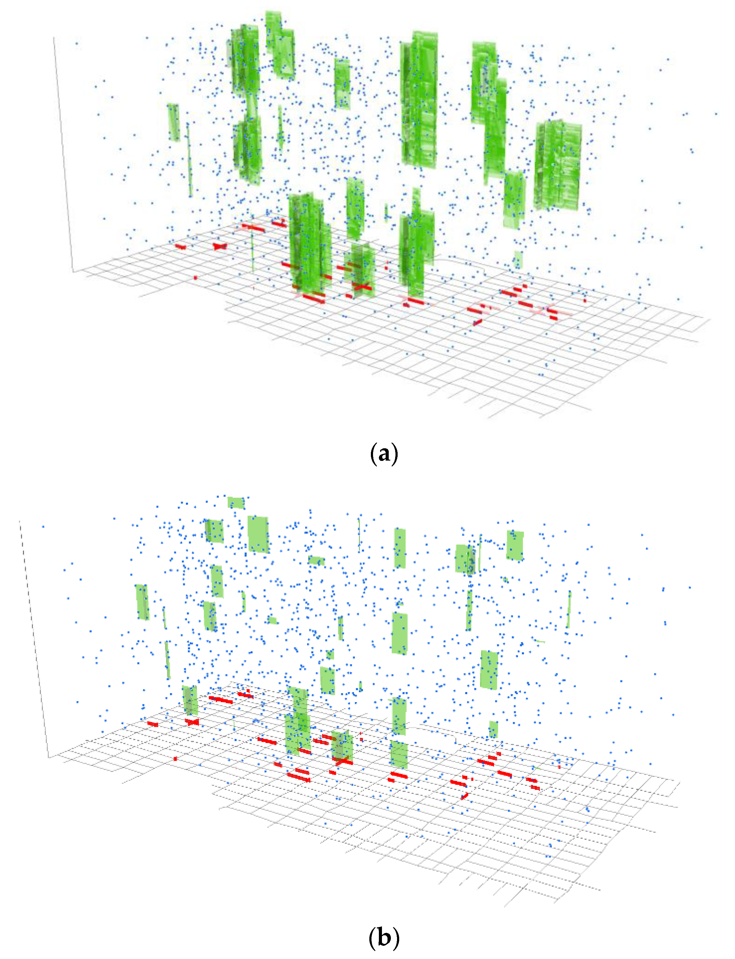
The images in Figure 7a,b give a three-dimensional view of the overlapping and non-overlapping space-time hotspots detected with NetScan, respectively. Overlapping hotspots were formed by all hotspots at that location whose likelihood ratios were statistically significant. A non-overlapping hotspot was a cluster with the highest likelihood ratio among those overlapped. The space-time coordinate of each crime incident is represented by a small blue dot in the space-time cube, shown at the intersection of the corresponding street address on the horizontal plane and the date of the year on the vertical axis. The space-time hotspots are illustrated with small patches of green rectangles covering concentrations of the space-time representation of crime incidents along the street network at a specific period of time during the year 2000.
The effect of visualising their temporal variation gives us a better understanding of when those hotspots emerged. The non-overlapping hotspots (Figure 7b) show the time and place of the “hottest” concentration of crime activities, whereas the overlapping hotspots reflect the concentration of multiple combinations of similar sets captured in a small space and time. In general, the extent of overlaps between those clusters seems greater in the spatial dimension and less on the temporal dimension. In other words, the overlapping clusters cover a similar spatial extent, but there is some variation in the period they have captured; i.e., clusters are detected across a period of time, collectively forming a combined cluster that is visibly longer than that of a single non-overlapping hotspot representing them. It can be considered as a sign of stability (stable hotbeds) that is clearly demarked in spatial terms, and crime activities are repeatedly observed across time in these locations, which translate into the multiple periods that are captured by the series of overlapping clusters. The non-overlapping hotspot that represents all of them can be considered as their champion, with the most intense spatial–temporal concentration, but the tail that follows (or the precursor that appears immediately before) can be, in practical terms, considered as part of the concentrated activities that took place there during that period.
6. Discussion
The simulation study (i.e., performance tests using synthetic data) demonstrated that the conventional Euclidean-based methods do not return strong performance when analysing point distributions that are constrained by a network structure, in the sense that they tend give inaccurate results by under-representing, overshooting or failing to detect problem places. The undershooting meant that some of the problem places were not identified correctly, while cases of overshooting resulted in the covering of an excessively wide area, including near-crime-free areas in the vicinity. These errors could actually worsen misunderstanding about problem places as well as about the risk factors that trigger crimes. The simulation study relied on a single pattern of a street network that was fairly regular in its configuration, and the results were not conclusive. However, because NetScan uses a search window that flexibly adopts the structure of a street network, its performance should be consistent regardless of the configuration of the street network. In contrast, the performances of the conventional methods are directly affected by the network configuration, and therefore, the comparative advantage of NetScan is likely to increase when detecting hotspots across more irregular networks.
In terms of the internal validity, no subjectivity exists with the synthetic data. As discussed in the manuscript, it adopts the widely-used Poisson cluster process to produce unbiased, random distribution. In order to test the performance over multiple clusters, we produced 14 clusters; this number was chosen simply because, through iterative exploration, we discovered that any more clusters would make it very difficult to prevent the test area from getting overly crowded with clusters. Furthermore, the association between the network and the points contained within is purely that of locational arrangements, and therefore, remains unchanged and unaffected; this is regardless of the type of data. This is because the analysis here relies purely on the locational data and no other attributes or weights are needed.
On the external validity, NetScan is robust and should be applicable to any form of network structure as long as it is defined on a two-dimensional plane. This is because, at the computational stage, a single network datum is reduced to a simple structure consisting of nodes and edges. Additionally, the data quantity (or the extent of the network), or the topological arrangement of the network (e.g., dimension of each edge, or the number streets that are connected at each junction) do not affect the computational process or the algorithm itself. For these reasons, variations in these parameters should not affect the validity of the method.
Empirical analyses revealed that drug incidents tend to be concentrated at specific places on a street. It confirms the recent criminological findings on crime and place—a large portion of crime incidents are known to concentrate on a limited number of streets and form hotspots at those locations. NetScan was effective in identifying when, where and to what extent crimes were forming such concentrations. The size of a micro-scale hotspot was occasionally smaller than that of a street segment, with some hotspots being detected between a handful of street addresses, while some other cases expanded over multiple street segments. In particular, the spatially overlapping hotspots in Figure 7a highlighted several small places on the street that saw a heavy recurrence of drug-related incidents across the duration of the study period. The flexibility in the size of NetScan’s search windows in both spatial and temporal dimensions not only helped identify hotspots of different sizes, but also clarified the space-time signature, namely the persistent and stable nature of drug incidents.
The difference in the size of crime hotspots can be considered to reflect the variability in the extent of environmental and situational factors. For instance, the presence of spot-like hotspots suggests that the crime determinant factors, along with crime opportunities created by these factors, may exist over a very small area in those places, separating the problem places from their immediate vicinity on a very fine scale. On the other hand, hotspots that cover a larger area indicate the prevalence of these factors across the entire length of the area, which collectively produces certain crime opportunities, and the unit of area should be adjusted accordingly. The flexibility in the temporal dimension (i.e., the capacity to change the temporal duration of the search windows for NetScan) is also important, as search windows with a short temporal size can detect short-term hotspots, whereas a search window with a longer temporal size can also detect hotspots that are long-lasting and persistent. The ability to detect different types of hotspots with search windows of different sizes helps in the investigation of situational factors during a period when crime opportunities are elevated at particular places.
7. Conclusions
This paper proposed a new type of method, NetScan, for detecting hotspots along a network over space and time. The foremost methodological advantage of the NetScan is in its increased accuracy for detecting crime hotspots, both in space and time. Using the network distance for the space-time searches of clusters is the key in detecting problem places at the street address level. In practice, the choice over NetScan and PLScan largely depends on the context. If we target the spatial–temporal patterns of events that are constrained to micro-scale and network-space, such as crimes in an urban area, NetScan provides a more accurate result. However, if the events are not affected by the street network (e.g., airborne disease that spreads in over a straight-line distance), PLScan may be a more suitable option. In the context of the geography of crime, NetScan helps us capture the space-time signature of a specific type of crime and find micro-scale crime-inducing factors that are present at a specific time and place. This in turn leads us to a better understanding of crime opportunity structures and the aetiology of crime—why crimes form a concentration at that particular place and time—which has recently been investigated at the street-segment or the sub-street-segment levels. The level of geographical and temporal granularity of this study fits this type of enquiry particularly well.
Although NetScan generally returns results with high precision, it is not perfect. For instance, NetScan was found to be very effective in reducing overshooting, but less so in controlling undershooting. The high computational load is also an issue that it shares with PLScan, especially when it comes to applying this method for micro-scale hotspot detection against a large space-time dataset. Improvement of the computational performance and further improvement in the detection accuracy marks a future avenue for research. However, NetScan and the outcome from this study expanded the possibilities for analysing crime incidents and crime opportunities at the micro-scale across space and time.
This paper was pursued in the context of crime-and-place studies. However, the proposed method is expected to make conceptual and methodological contributions beyond the analysis of drug-related crimes. Its applications need not be constrained to the fields of geography and criminology, as the principle of detecting micro-scale concentrations is fundamentally applicable to any context. NetScan could make a difference in other disciplines of natural and social sciences that involve analyses of concentrations on a network. Examples include traffic accident analysis in the field of transportation planning and policy, as well as epidemiological applications, such as the identification of a micro-level disease outbreak in an urban environment.
Author Contributions
Conceptualization, S.S. and N.S.; methodology, S.S. and N.S.; software, S.S.; validation, S.S. and N.S.; formal analysis, S.S.; investigation, S.S. and N.S.; data curation, S.S.; writing—original draft preparation, S.S. and N.S.; writing—review and editing, N.S. and S.S.; visualization, S.S. and N.S. All authors have read and agreed to the published version of the manuscript.
Funding
This research received no external funding.
Institutional Review Board Statement
Not applicable.
Informed Consent Statement
Not applicable.
Data Availability Statement
The crime data used in the empirical analysis can be found at the Chicago Data Portal https://data.cityofchicago.org/Public-Safety/Crimes-2001-to-Present/ijzp-q8t2 accessed on 1 October 2022.
Conflicts of Interest
The authors declare no conflict of interest.
References
- Chorley, R.J.; Haggett, P. (Eds.) Models in Geography; Methuen: London, UK, 1967. [Google Scholar]
- Clark, P.J.; Evans, F.C. Distance to nearest neighbor as a measure of spatial relationships in populations. Ecology 1954, 35, 445–453. [Google Scholar] [CrossRef]
- Diggle, P.J.; Besag, J.; Gleaves, J.T. Statistical analysis of spatial point patterns by means of distance methods. Biometrics 1976, 32, 659–667. [Google Scholar] [CrossRef]
- Ripley, B.D. The second-order analysis of stationary point process. J. Appl. Probab. 1976, 13, 255–266. [Google Scholar] [CrossRef] [Green Version]
- Ripley, B.D. Spatial Statistics; John Wiley & Sons: New York, NY, USA, 1981. [Google Scholar]
- Boots, B.N.; Getis, A. Point Pattern Analysis; Sage Publications: Thousand Oaks, CA, USA, 1988. [Google Scholar]
- Knox, E.G. Detection of clusters. In Methodology of Enquiries into Disease Clustering; Elliott, P., Ed.; Small Area Health Statistics Unit: London, UK, 1989; pp. 17–20. [Google Scholar]
- Kulldorff, M.; Nagarwalla, N. Spatial disease clusters: Detection and inference. Stat. Med. 1995, 14, 799–810. [Google Scholar] [CrossRef]
- Rogerson, P.A. Monitoring point patterns for the development of spacetime clusters. J. R. Stat. Soc. Ser. A Stat. Soc. 2001, 164, 87–96. [Google Scholar] [CrossRef]
- Weisburd, D.; Bushway, S.; Lum, C.; Yang, S.-M. Trajectories of crime at places: A longitudinal study of street segments in the city of Seattle. Criminology 2004, 42, 283–321. [Google Scholar] [CrossRef]
- Braga, A.A.; Papachristos, A.V.; Hureau, D.M. The concentration and stability of gun violence at micro places in Boston, 1980–2008. J. Quant. Criminol. 2010, 26, 33–53. [Google Scholar] [CrossRef]
- Weisburd, D.; Telep, C.W. Hot spots policing: What we know and what we need to know. J. Contemp. Crim. 2014, 30, 200–220. [Google Scholar] [CrossRef]
- Lee, Y.; Eck, J.E.; Martinez, N.N. How concentrated is crime at places? A systematic review from 1970 to 2015. Crime Sci. 2017, 6, 6. [Google Scholar] [CrossRef]
- Oliveira, M.; Bastos-Filho, C.; Menezes, R. The scaling of crime concentration in cities. PLoS ONE 2017, 12, e0183110. [Google Scholar] [CrossRef]
- Mohler, G.; Porter, M.; Carter, J.; LaFree, G. Learning to rank spatio-temporal event hotspots. Crime Sci. 2020, 9, 3. [Google Scholar] [CrossRef] [Green Version]
- Weisburd, D. The law of crime concentration and the criminology of place. Criminology 2015, 53, 133–157. [Google Scholar] [CrossRef]
- O’Brien, D.; Winship, C. The Gains of Greater Granularity: The Presence and Persistence of Problem Properties in Urban Neighborhoods. J. Quant. Criminol. 2017, 33, 649–674. [Google Scholar] [CrossRef]
- Robinson, A.H. Early Thematic Mapping in the History of Cartography; University of Chicago Press: Chicago, IL, USA, 1982. [Google Scholar]
- Evans, D.J.; Herbert, D.T. The Geography of Crime; Routledge: London, UK, 1989. [Google Scholar]
- Weisburd, D.; McEwen, T. Crime Mapping and Crime Prevention; Criminal Justice Press: New York, NY, USA, 1998. [Google Scholar]
- Braga, A.A.; Weisburd, D.L. Editors’ introduction: Empirical evidence on the relevance of place in criminology. J. Quant. Criminol. 2010, 26, 1–6. [Google Scholar] [CrossRef] [Green Version]
- Braga, A.A.; Papachristos, A.V.; Hureau, D.M. The effects of hot spots policing on crime: An updated systematic review and meta-analysis. Justice Q. 2014, 31, 633–663. [Google Scholar] [CrossRef]
- Weisburd, D.; Groff, E.R.; Yang, S. The Criminology of Place: Street Segments and Our Understanding of The Crime Problem; Oxford University Press: New York, NY, USA, 2012. [Google Scholar]
- Braga, A.A. The effects of hot spots policing on crime. Ann. Am. Acad. Pol. Soc. Sci. 2001, 455, 104–125. [Google Scholar] [CrossRef]
- Weisburd, D.; Eck, J. What can police do to reduce crime, disorder and fear? Ann. Am. Acad. Pol. Soc. Sci. 2004, 593, 42–65. [Google Scholar] [CrossRef]
- Weisburd, D.; Braga, A. Hot spots policing as a model for police innovation. In Police Innovation: Contrasting Perspectives; Weisburd, D., Braga, A., Eds.; Cambridge University Press: Cambridge, UK, 2006; pp. 225–244. [Google Scholar]
- Weisburd, D.; Morris, N.A.; Groff, E.R. Hot spots of juvenile crime: A longitudinal study of arrest incidents at street segments in Seattle, Washington. J. Quant. Criminol. 2009, 25, 443–467. [Google Scholar] [CrossRef]
- Dau, P.M.; Dewinter, M.; Witlox, F.; Vander Beken, T.; Vandeviver, C. How concentrated are police on crime? A spatiotemporal analysis of the concentration of police presence and crime. Camb. J. Evid.-Based Polic. 2022. [Google Scholar] [CrossRef]
- Braga, A.A.; Turchan, B.S.; Papachristos, A.V.; Hureau, D.M. Hot spots policing and crime reduction: An update of an ongoing systematic review and meta-analysis. J. Exp. Criminol. 2019, 15, 289–311. [Google Scholar] [CrossRef]
- Braga, A.A.; Hureau, D.; Winship, C. Losing faith? Police, black churches, and the resurgence of youth violence in Boston. Ohio State J. Crim. Law 2008, 6, 141–172. [Google Scholar]
- Weisburd, D.; Zastrow, T. Crime Hot Spots: A Study of New York City Streets in 2010, 2015, and 2020, Report to Manhattan Institute 2021. Available online: https://www.manhattan-institute.org/weisburd-zastrow-crime-hot-spots (accessed on 1 November 2022).
- Eck, J. Review essay: Examining routine activity theory. Justice Q. 1995, 12, 783–797. [Google Scholar] [CrossRef]
- Eck, J.E.; Weisburd, D. Crime places in crime theory. In Crime and Place; Eck., J., Weisburd, D., Eds.; Crime Justice Press: Monsey, NY, USA, 1995; pp. 1–33. [Google Scholar]
- Sherman, L.W. Hot spots of crime and criminal careers of places. In Crime and Place. Crime Prevention Studies; Eck, J., Weisburd, D., Eds.; Willow Tree Press: Monsley, NY, USA, 1995; Volume 4, pp. 35–52. [Google Scholar]
- Taylor, R. Social order and disorder of street-blocks and neighborhoods: Ecology, micro-ecology, and the systematic model of social disorganization. J. Res. Crime Delinq. 1997, 34, 113–155. [Google Scholar] [CrossRef]
- Taylor, R. Crime in Small-Scale Places: What We Know, What We Can Prevent and What Else We Need to Know. In Crime and Place: Plenary Papers of the 1997 Conference on Criminal Justice Research and Evaluation; Travis, J., Ed.; U.S. National Institute of Justice: Washington, DC, USA, 1998. [Google Scholar]
- Van Wilsem, J. Urban streets as micro contexts to commit violence. In Putting Crime in Its Place: Units of Analysis in Geographic Criminology; Weisburd, D., Bernasco, W., Bruinsma, G.J.N., Eds.; Springer Verlag: New York, NY, USA, 2009. [Google Scholar]
- Di Bella, E.; Corsi, M.; Leporatti, L.; Persico, L. The spatial configuration of urban crime environments and statistical modeling. Environ. Plan. B Plann. Des. 2017, 44, 647–667. [Google Scholar] [CrossRef]
- Brantingham, P.L.; Brantingham, P.J. Theoretical model of crime hot spot generation. Stud. Crime Crime Prev. 1999, 8, 7–26. [Google Scholar]
- Bowers, K.J.; Johnson, S.D. Domestic burglary repeats and space-time clusters. Eur. J. Criminol. 2005, 2, 67–92. [Google Scholar] [CrossRef]
- Okabe, A.; Satoh, T. Spatial analysis on a network. In The SAGE Handbook on Spatial Analysis; Fotheringham, A.S., Rogerson, P.A., Eds.; Sage Publications: London, UK, 2009; pp. 443–464. [Google Scholar]
- Newton, A.; Felson, M. Editorial: Crime patterns in time and space: The dynamics of crime opportunities in urban areas. Crime Sci. 2015, 4, 11. [Google Scholar] [CrossRef] [Green Version]
- Braga, A.A.; Hureau, D.M.; Papachristos, A.V. The relevance of micro places to citywide robbery trends: A longitudinal analysis of robbery incidents at street corners and block faces in Boston. J. Res. Crime Delinq. 2011, 48, 7–32. [Google Scholar] [CrossRef]
- Groff, E.R.; Weisburd, D.; Yang, S.M. Is it important to examine crime trends at a local “micro” level?: A longitudinal analysis of street to street variability in crime trajectories. J. Quant. Criminol. 2010, 26, 7–32. [Google Scholar] [CrossRef]
- Levin, A.; Rosenfeld, R.; Deckard, M. The Law of Crime Concentration: An Application and Recommendations for Future Research. J. Quant. Criminol. 2017, 33, 635–647. [Google Scholar] [CrossRef]
- Johnson, S.; Bernasco, W.; Bowers, K.; Elffers, H.; Ratcliffe, J.; Rengert, G.; Townsley, M. Space-time patterns of risk: A cross national assessment of residential burglary victimization. J. Quant. Criminol. 2007, 23, 201–219. [Google Scholar] [CrossRef] [Green Version]
- Johnson, S.D.; Lab, S.P.; Bowers, K.J. Stable and fluid hotspots of crime: Differentiation and identification. Built Environ. 2008, 34, 32–45. [Google Scholar] [CrossRef]
- Brunsdon, C.; Corcoran, J.; Higgs, G. Visualising space and time in crime patterns: A comparison of methods. Comput. Environ. Urban Syst. 2007, 31, 52–75. [Google Scholar] [CrossRef]
- Neill, D.B.; Gorr, W.L. Detecting and preventing emerging epidemics of crime. Adv. Dis. Surveill. 2007, 4, 13. [Google Scholar]
- Nakaya, T.; Yano, K. Visualising crime clusters in a space-time cube: An exploratory data analysis approach using space-time kernel density estimation and scan statistics. Trans. GIS 2010, 14, 223–239. [Google Scholar] [CrossRef]
- Malleson, N.; Andresen, M.A. Spatio-temporal crime hotspots and the ambient population. Crime Sci. 2015, 4, 10. [Google Scholar] [CrossRef] [Green Version]
- Okabe, A.; Sugihara, K. Spatial Analysis along Networks: Statistical and Computational Methods; John Wiley & Sons: Chichester, UK, 2012. [Google Scholar]
- Okabe, A.; Satoh, T.; Sugihara, K. A kernel density estimation method for networks, its computational method and a GIS-based tool. Int. J. Geogr. Inf. Sci. 2009, 23, 7–32. [Google Scholar] [CrossRef]
- Yamada, I.; Thill, J.C. Local indicators of network-constrained clusters in spatial patterns represented by a link attribute. Ann. Am. Assoc. Geogr. 2010, 100, 269–285. [Google Scholar] [CrossRef]
- Nie, K.; Wang, Z.; Du, Q.; Ren, F.; Tian, Q. A network-constrained integrated method for detecting spatial cluster and risk location of traffic crash: A case study from Wuhan, China. Sustainability 2015, 7, 2662–2677. [Google Scholar] [CrossRef] [Green Version]
- Rosser, G.; Davies, T.; Bowers, K.; Johnson, S.; Cheng, T. Predictive Crime Mapping: Arbitrary Grids or Street Networks? J. Quant. Criminol. 2017, 33, 569–594. [Google Scholar] [CrossRef] [PubMed] [Green Version]
- Shiode, S.; Shiode, N. Network-based space-time search window technique for hotspot detection of street-level crime incidents. Int. J. Geogr. Inf. Sci. 2013, 27, 866–882. [Google Scholar] [CrossRef]
- Shiode, S.; Shiode, N.; Block, R.; Block, C. Space-time characteristics of micro-scale crime occurrences: An application of a network-based space-time search window technique for crime incidents in Chicago. Int. J. Geogr. Inf. Sci. 2015, 29, 697–719. [Google Scholar] [CrossRef]
- Bonferroni, C.E. Il calcolo delle assicurazioni su gruppi di teste. In Studi in Onore del Professore Salvatore Ortu Carboni; Bardi: Rome, Italy, 1935; pp. 13–60. [Google Scholar]
- Benjamini, Y.; Hochberg, Y. Controlling the false discovery rate: A practical and powerful approach to multiple testing. J. R. Stat. Soc. Ser. B Stat. Methodol. 1995, 57, 289–300. [Google Scholar] [CrossRef]
- Kulldorff, M. A spatial scan statistic. Commun. Stat. 1997, 26, 1481–1496. [Google Scholar] [CrossRef]
- Cheng, T.; Adepeju, M. Modifiable Temporal Unit Problem (MTUP) and its effect on space-time cluster detection. PLoS ONE 2014, 9, e100465. [Google Scholar] [CrossRef] [PubMed] [Green Version]
- Duczmal, L.; Kulldorff, M.; Huang, L. Evaluation of spatial scan statistics for irregularly shaped clusters. J. Comput. Graph. Stat. 2006, 15, 428–442. [Google Scholar] [CrossRef]
- Neill, D.B. Expectation-based Scan Statistics for monitoring spatial time series data. Int. J. Forecast. 2009, 25, 498–517. [Google Scholar] [CrossRef] [Green Version]
- Assunção, R.; Costa, M.; Tavares, A.; Ferreira, S. Fast detection of arbitrarily shaped disease clusters. Stat. Med. 2006, 25, 723–742. [Google Scholar] [CrossRef]
- Kulldorff, M. SaTScan User Guide Version 10.1. 2022. Available online: https://www.satscan.org/cgi-bin/satscan/register.pl/SaTScan_Users_Guide.pdf?todo=process_userguide_download (accessed on 1 November 2022).
- Upton, G.J.G.; Fingleton, B. Spatial Data Analysis by Example; John Wiley & Sons: Chichester, UK, 1985. [Google Scholar]
- Diggle, P.J. Statistical Analysis of Spatial Point Patterns; Oxford University Press: New York, NY, USA, 2003. [Google Scholar]
- Kulldorff, M.; Athas, W.; Feuer, E.; Miller, B.; Key, C. Evaluating cluster alarms: A space-time scan statistic and brain cancer in Los Alamos. Am. J. Public Health 1998, 88, 1377–1380. [Google Scholar] [CrossRef] [Green Version]
- Okabe, A.; Okunuki, K.; Shiode, S. SANET: A Toolbox for Spatial Analysis on a Network Version 3.4.1. 2009. Available online: http://sanet.csis.u-tokyo.ac.jp/download/manual_ver3.pdf (accessed on 1 November 2022).
- Nordin, J.D.; Goodman, M.J.; Kulldorff, M.; Ritzwoller, D.P.; Abrams, A.M.; Kleinman, K. Simulated anthrax attacks and syndromic surveillance. Emerg. Infect. Dis. 2005, 11, 1394–1398. [Google Scholar] [CrossRef]
- Forsberg, L.; Bonetti, M.; Jeffery, C.; Ozonoff, A.; Pagano, M. Distance-based methods for spatial and spatio-temporal surveillance. In Spatial & Syndromic Surveillance for Public Health, 2nd ed.; Lawson, A.B., Kleinman, K., Eds.; Wiley & Sons: Chichester, UK, 2005; pp. 115–131. [Google Scholar]
- Huang, L.; Kulldorff, M.; Gregorio, D. A spatial scan statistic for survival data. Biometrics 2007, 63, 109–118. [Google Scholar] [CrossRef] [PubMed] [Green Version]
- Takahashi, K.; Kulldorff, M.; Tango, T.; Yih, K. A flexibly shaped space-time scan statistic for disease outbreak detection and monitoring. Int. J. Health Geogr. 2008, 7, 14. [Google Scholar] [CrossRef] [PubMed] [Green Version]
- Sherman, L.W.; Weisburd, D. General deterrent effects of police patrol in crime hot-spots: A randomized, controlled trial. Justice Q. 1995, 12, 625–648. [Google Scholar] [CrossRef]
- Weisburd, D.; Green, L. Policing drug hot spots: The Jersey City drug market analysis experiment. Justice Q. 1995, 12, 711–735. [Google Scholar] [CrossRef]
- Jacobson, J. Policing Drug Hot-Spots: The Situational Approach; Police Research Series Paper 109; Home Office Policing and Reducing Crime Unit: London, UK, 1999.
- Mazerolle, L.; Soole, D.W.; Rombouts, S. Crime Prevention Research Reviews No.1: Disrupting Street-Level Drug Markets; U.S. Department of Justice, Office of Community Oriented Policing Services: Washington, DC, USA, 2007.
- Braga, A.A.; Bond, B.J. Policing crime and disorder hot spots: A randomized controlled trial. Criminology 2008, 46, 577–608. [Google Scholar] [CrossRef]
Figure 1.
ID numbers assigned to the 14 simulated hotspots.
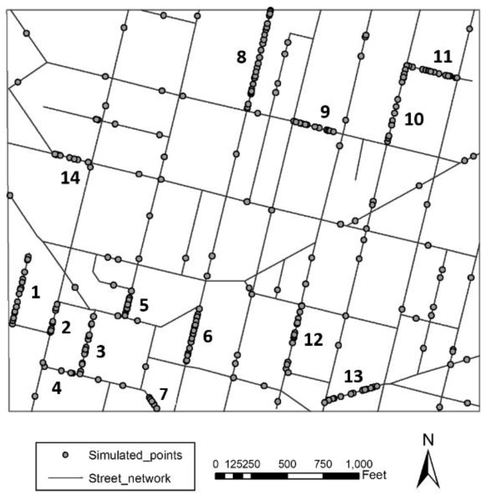
Figure 2.
Simulated space-time Poisson cluster points presented in a space-time cube.
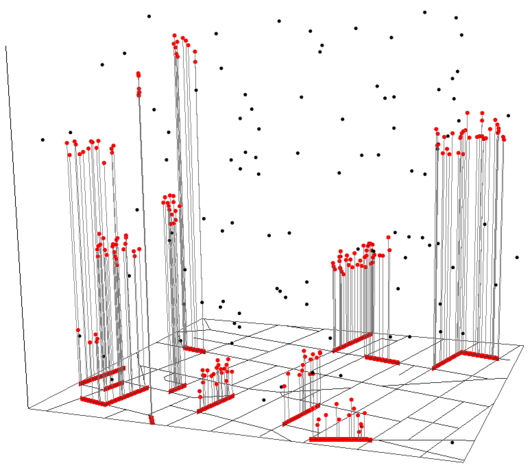
Figure 3.
The most likely and the secondary non-overlapping space-time hotspots detected with circular PLScan.
Figure 3.
The most likely and the secondary non-overlapping space-time hotspots detected with circular PLScan.

Figure 4.
The most likely and the secondary non-overlapping space-time hotspots detected with elliptic PLScan.
Figure 4.
The most likely and the secondary non-overlapping space-time hotspots detected with elliptic PLScan.
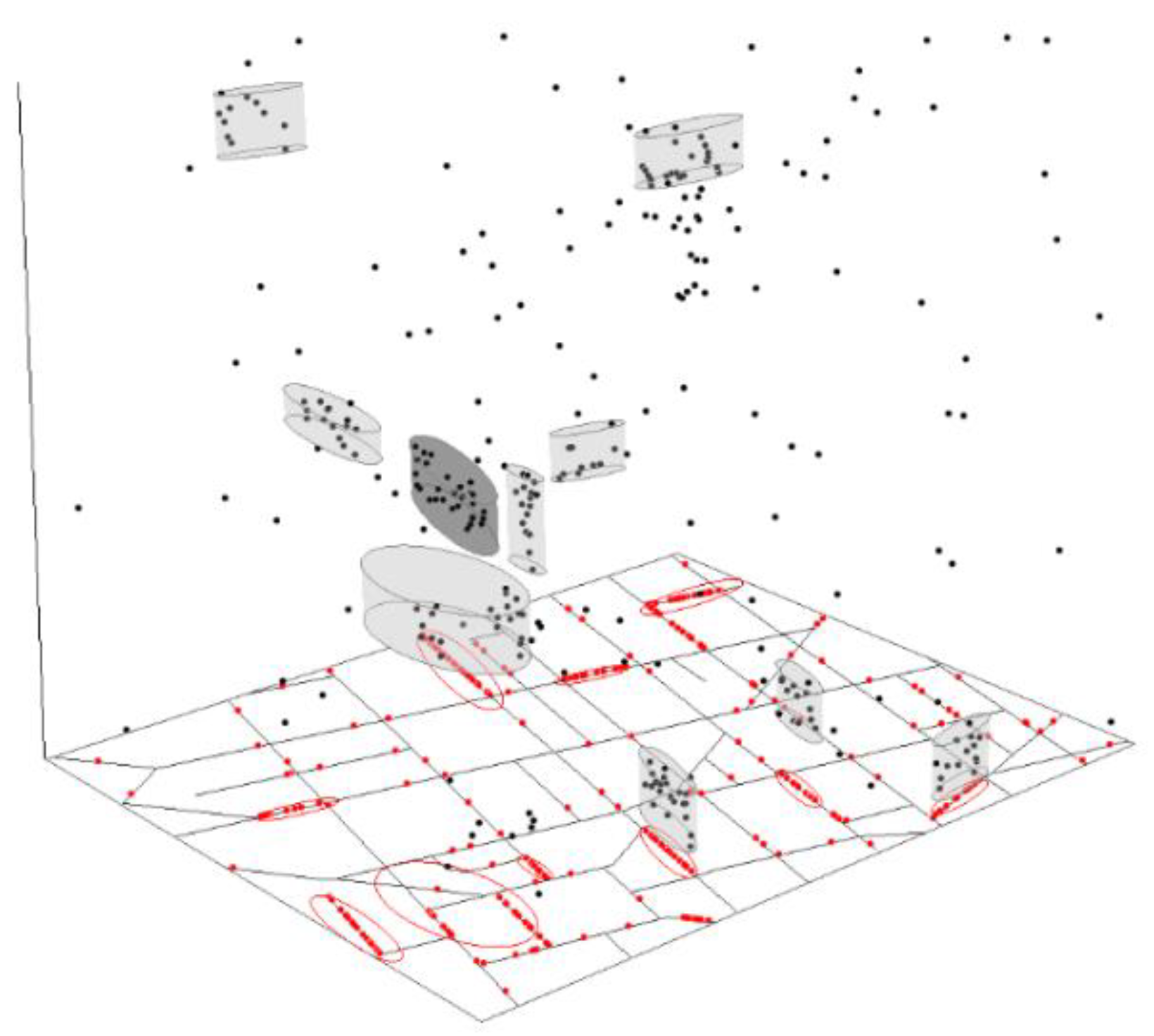
Figure 5.
The most likely and the secondary non-overlapping space-time hotspots detected with NetScan.
Figure 5.
The most likely and the secondary non-overlapping space-time hotspots detected with NetScan.
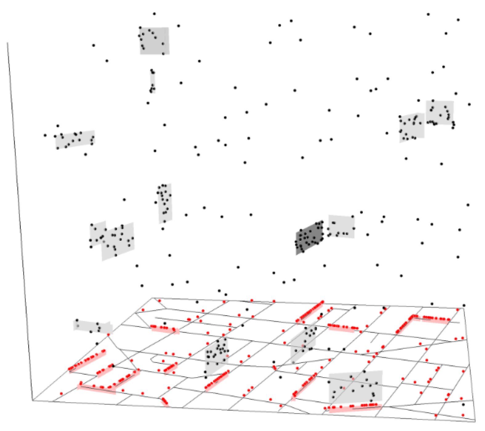
Figure 6.
(a) Spatial hotspots and (b) space-time hotspots of drug offences in Englewood, Chicago IL in 2000.
Figure 6.
(a) Spatial hotspots and (b) space-time hotspots of drug offences in Englewood, Chicago IL in 2000.
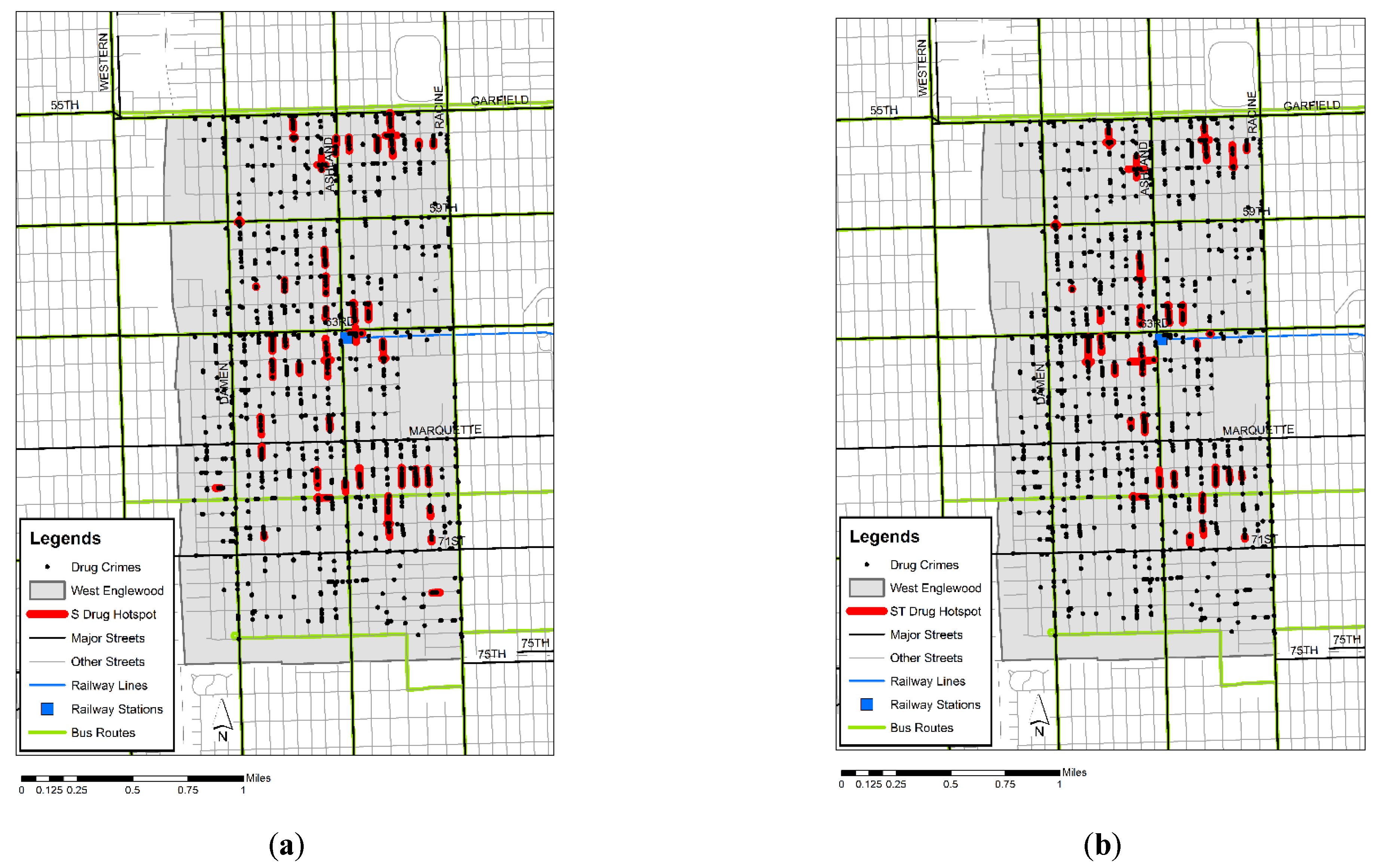
Figure 7.
Projection of (a) the overlapping and (b) the non-overlapping space-time hotspots of drug offences in Englewood, Chicago IL in 2000.
Figure 7.
Projection of (a) the overlapping and (b) the non-overlapping space-time hotspots of drug offences in Englewood, Chicago IL in 2000.

Table 1.
The period and the size of the 14 space-time hotspots.
| Hotspot ID | Start Date | End Date | Number of Events |
|---|---|---|---|
| 1 | 221 | 251 | 15 |
| 2 | 135 | 165 | 8 |
| 3 | 130 | 160 | 16 |
| 4 | 59 | 89 | 5 |
| 5 | 167 | 197 | 14 |
| 6 | 12 | 42 | 21 |
| 7 | 288 | 318 | 8 |
| 8 | 84 | 114 | 30 |
| 9 | 109 | 139 | 10 |
| 10 | 227 | 257 | 15 |
| 11 | 242 | 272 | 19 |
| 12 | 34 | 64 | 14 |
| 13 | 7 | 37 | 14 |
| 14 | 327 | 357 | 11 |
Table 2.
Comparison of the extent of coverage by circular PLScan, elliptic PLScan and NetScan.
| PPV | Sensitivity | |
|---|---|---|
| Circular PLScan | 0.23 | 0.62 |
| Elliptic PLScan | 0.74 | 0.65 |
| NetScan | 0.99 | 0.88 |
Publisher’s Note: MDPI stays neutral with regard to jurisdictional claims in published maps and institutional affiliations. |
© 2022 by the authors. Licensee MDPI, Basel, Switzerland. This article is an open access article distributed under the terms and conditions of the Creative Commons Attribution (CC BY) license (https://creativecommons.org/licenses/by/4.0/).
Share and Cite
MDPI and ACS Style
Shiode, S.; Shiode, N. Network-Based Space-Time Scan Statistics for Detecting Micro-Scale Hotspots. Sustainability 2022, 14, 16902. https://doi.org/10.3390/su142416902
AMA Style
Shiode S, Shiode N. Network-Based Space-Time Scan Statistics for Detecting Micro-Scale Hotspots. Sustainability. 2022; 14(24):16902. https://doi.org/10.3390/su142416902
Chicago/Turabian StyleShiode, Shino, and Narushige Shiode. 2022. "Network-Based Space-Time Scan Statistics for Detecting Micro-Scale Hotspots" Sustainability 14, no. 24: 16902. https://doi.org/10.3390/su142416902
Note that from the first issue of 2016, this journal uses article numbers instead of page numbers. See further details here.