
A Supervised Machine Learning Classification Framework for Clothing Products’ Sustainability


Louvain Research Institute in Management and Organizations (LouRIM), UCLouvain, 7000 Mons, Belgium
*
Author to whom correspondence should be addressed.
Sustainability 2022, 14(3), 1334; https://doi.org/10.3390/su14031334
Submission received: 30 December 2021
/
Revised: 15 January 2022
/
Accepted: 19 January 2022
/
Published: 25 January 2022
(This article belongs to the Special Issue Machine Learning and AI Technology for Sustainability)
Abstract
:These days, many sustainability-minded consumers face a major problem when trying to identify environmentally sustainable products. Indeed, there are a variety of confusing sustainability certifications and few labels capturing the overall environmental impact of products, as the existing procedures for assessing the environmental impact of products throughout their life cycle are time consuming, costly, and require a lot of data and input from domain experts. This paper explores the use of supervised machine learning tools to extrapolate the results of existing life cycle assessment studies (LCAs) and to develop a model—applied to the clothing product category—that could easily and quickly assess the products’ environmental sustainability throughout their life cycle. More precisely, we assemble a dataset of clothing products with their life cycle characteristics and corresponding known total environmental impact and test, on a 5-fold cross-validation basis, nine state-of-the-art supervised machine learning algorithms. Among them, the random forest algorithm has the best performance with an average accuracy of 91% over the five folds. The resulting model provides rapid environmental feedback on a variety of clothing products with the limited data available to online retailers. It could be used to quickly provide interested consumers with product-level sustainability information, or even to develop a unique and all-inclusive environmental label.
1. Introduction and Related Work
Our current consumption pattern is a major cause of damage to the natural environment (see, e.g., [1]). The consumption of fashion products in particular has changed with the emergence of fast fashion—the sale of cheap and widely available garments—as a dominant business model. As shown in [2,3], our current fashion consumption has a disastrous impact on the environment: indeed, the fashion industry accounts for around 10% of carbon emissions of human activity, it is the second-largest consumer of water, it uses massive amounts of energy, it produces a lot of waste, and it pollutes water and soil with microplastics and chemicals. Following [2], a change in clothing buying habits could be a first step in the right direction. A growing number of consumers seems to be aware of this issue and willing to make efforts to limit their consumption and adopt proenvironmental consumption habits (see, e.g., [4,5]). References [6,7] mention there is however an intention–behavior gap, as many consumers find environment-friendly products too little highlighted and hard to find, but also as consumers are confused about the many environmental labels, are suspicious of companies’ environmental claims, and lack clear information on the overall environmental impact of products. The fashion industry for instance indeed lacks a clear environmental labeling system. Sustainability-minded consumers consequently face a major problem when trying to identify environmentally sustainable products. As highlighted in [8,9], there are a variety of confusing sustainability certifications and few labels capturing the overall environmental impact of products, as the existing procedures for assessing the environmental impact of products throughout their life cycle are time consuming, costly, and require a lot of data and input from domain experts.
To define whether a product is environmentally sustainable and can be labeled as such, it is necessary to appraise the environmental impact of the product over its entire life cycle (see, e.g., [10]). A widely recognized method for assessing the effects that a product has on the environment throughout its life is the life cycle assessment (LCA) method. The LCA method assesses the environmental impacts of a product from the raw material extraction and processing (cradle), through the product’s manufacture, distribution and use, to its recycling or final disposal (grave) (see, e.g., [11]). A LCA study typically includes (1) a life cycle inventory (LCI) phase, i.e., a thorough inventory of the required energy, materials, etc., for a product from cradle to grave and (2) a life cycle impact assessment (LCIA) phase, i.e., the assessment of the environmental impacts of these inventory components. LCA studies generally rely on large databases (e.g., GaBi database, Ecoinvent), built by domain experts, containing the environmental impact of various product components and processes. Calculations of the impact of all the environmental loads associated to a product can then be performed using a simple spreadsheet or with LCA tools and software solutions (e.g., GaBi and SimaPro). Some tools allow one to conduct LCA procedures for specific industries (e.g., the LCA-based Higg Product Tools for the apparel industry). The LCA method is increasingly used for product labeling and for environmental product declarations (EPDs). However, as LCA procedures are complex, time consuming, and costly, it is difficult to use this method to quickly assign an all-inclusive environmental sustainability score to products. Consequently, at the time of this study, there are a lot of—even too many—different environmental labels that only consider certain aspects of the life cycle, instead of having a single label capturing the overall environmental impact of products throughout their entire life cycle.
As machine learning techniques have evolved, they have been increasingly used to address sustainability issues. Outside of LCA, applications of machine learning have included, for example, generating models predicting hailstorms [12] or defects in industrial equipment [13]. In the field of LCA, researchers have begun to exploit machine learning techniques to reduce the costs and time required for LCA studies [14]. Machine learning has been used in LCAs to estimate values for environmental impact characterization factors, to perform sensitivity analyses, or to develop frameworks for predicting the environmental impact of products over their entire life cycle. These surrogate LCAs provide approximate results but avoid a complex and time consuming procedure. This way, in the early 2000s, refs. [15,16,17,18] trained a neural network, using a database of LCA results mapped to design-phase product attributes of household appliances, to generalize the relationships between product attributes and LCA indicators, and to provide predictions of LCA indicators for new product descriptions. Similarly, ref. [19] trained multilayer artificial neural networks to estimate the impacts of chemicals over their entire life cycle. References [20,21] rather proposed to automate the process of assigning environmental impact factors to inventory components of a product. The authors consider the environmental impact assessment as a similarity problem, i.e., if an environmental dataset is structured as a matrix where the rows correspond to the components and the columns to the impact factors, expeditious environmental impact assessment is possible by matching a given life cycle inventory component to similar environmental database elements. In 2012, ref. [22] developed a software to apply the carbon footprint to a packaged consumer goods company’s large product portfolio in a short time. The final predictive model generates estimated emission factors for materials, thereby eliminating the manual mapping of a product’s inventory to environmental databases.
Our Work and Contribution
Using machine learning tools to find a model that could easily and quickly assess the sustainability of a large number of products throughout their life cycle has however not yet been tested for all product categories (e.g., clothing products instead of household appliances or chemicals) or for more specific contexts (e.g., for use by online retailers instead of product designers). In this paper, we seek to develop a model that could easily and quickly assess the environmental sustainability of clothing products with the limited data available to online retailers. Our motivations and contributions are manifold:
- Provide online retailers with a tool to easily and quickly assess the environmental sustainability of the clothing products in their catalog;
- Help consumers identify sustainable clothing products and close the intention–behavior gap in purchasing sustainable products;
- Provide a basis for the development of a label reflecting more comprehensively (i.e., more than the current sustainability certifications) the environmental sustainability of clothing products;
- Explore the potential of machine learning techniques for contributing to sustainable development;
- Provide a dataset that could be used for further research on the sustainability of clothing products.
Section 2 describes the methodology and the nine supervised machine learning algorithms tested for modeling the relationship between the sustainability of clothing products and the components and processes involved in their life cycle. The performance and capabilities of the formed models are presented in Section 3 and discussed in Section 4. Section 5 concludes the paper by presenting possible improvements to the models and suggestions for further work.
2. Materials and Methods
To build an environmental impact assessment model, we applied supervised machine learning techniques on a classification problem. Supervised machine learning involves training and learning a model from patterns that can be identified in a dataset with training examples that are pairs consisting of an input object and an output variable, so that the learned model can predict the output variable for new input data (see, e.g., [23]). The obtained model is often evaluated using input–output pairs that were not used for training the model, by comparing the outputs from the model to the desired outputs. We more particularly tackled a classification problem. In a classification problem, the output variable is categorical, and the obtained model attempts to predict how a new input object should be labeled.
In Section 2.1, we present the dataset assembled based on previously conducted LCA studies, containing clothing products (observations), their life cycle characteristics (independent input variables or features), and the corresponding total environmental impact (dependent output variable or outcome variable). We applied a stratified 5-fold cross-validation procedure, i.e., we divided the dataset into five nonoverlapping folds, and used each fold (20% of the data) once as a held back test set whilst all other folds collectively (80% of the data) were used as training set. We thus fitted and evaluated a model on five different data subsets for each machine learning algorithm and reported the average performance over the five iterations to estimate the overall performance of the algorithm (see, e.g., [23]). In Section 2.2, we present the nine machine learning algorithms applied to training data to find a function or set of rules that models the data with the least error. The metrics used for assessing the models and algorithms are presented in Section 2.3. Each machine learning algorithm includes one or more hyperparameters that allow the algorithm behavior to be tailored to the specificities of a dataset. To configure the hyperparameters to our dataset, a grid search optimization procedure with crossvalidation is used. Consequently, we applied a double crossvalidation: we used one crossvalidation procedure to estimate and compare the performance of different machine learning models, and one to evaluate and compare the performance of sets of model hyperparameters. To overcome the problem of overfitting, we nested the (inner) hyperparameter optimization procedure under the (outer) model selection procedure, as suggested by [23].
2.1. Data Collection and Pretreatment
Building the dataset required (1) selecting a meaningful set of product attributes as features, (2) collecting previously life-cycle-analyzed clothing products, and (3) defining the outcome variable, as detailed in this section.
2.1.1. Selection of the Features
The selected life cycle characteristics inputs should logically and statistically be linked to environmental impact data but should also be product attributes accessible to online retailers, so that they can apply the model to their product catalog. Therefore, we first formed a set of candidate product attributes based upon the literature and the experience of experts regarding the clothing supply chain, which we then refined using different criteria, to create a set of meaningful features. The main criteria used for selecting product attributes to use as features are their relationship to various factors impacting the environment (e.g., energy consumption, garment recyclability, etc.) and their accessibility to online retailers.
The clothing supply chain begins with the production of fibers, followed by spinning to produce yarn. Fabrics are manufactured from yarns through knitting or weaving. After bleaching and dyeing, the garment is manufactured by cutting, sewing, and adding trims. After manufacturing, the garments are shipped to central distribution centers and eventually to smaller retailers. The garments are used, and, at the end of their life, they are incinerated, transported to landfills or developing countries, and few are recycled. As shown in [3], a garment has an impact on the environment at each stage of its supply chain. According to [24], most of the life cycle impacts of apparel products occur in the use and production phases. The impacts on water resources, carbon emissions, waste, and chemical pollution vary by garment type as those with higher mass or volume require more resources, for instance (see, e.g., [3]). However, these impacts vary even for the same garment type, depending on different choices made throughout the life cycle, such as the fiber chosen, which has an impact on the natural resources, water, energy, and chemicals used throughout the manufacturing phase but also on the biodegradability and recyclability of the garment at its end-of-life. According to the sustainable brand Reformation [25], the raw materials could determine up to two-thirds of the impact of a garment. As also shown by [26], the process technology and equipment used during the cultivation and manufacturing phases also have an impact on the amount of waste produced and on the amount of energy, water, and chemicals used. Where the garment is manufactured is also determinant, as some countries have better environmental regulations and rely on more renewable energy sources. The location of the garment production also influences the distance the garment travels around the globe and can indirectly impact the transportation means, which in turn influence carbon emissions. The impact of the use phase varies depending on factors such as consumer behavior, the technologies used, and the geographical zone in which the product is used. The type of washing and drying required by the garment during its use-time, which partly depends on the type of fiber used, also has an impact on the water and energy required during the use phase. Finally, specific end-of-life instructions might impact the decision to dispose of the garment in a landfill or to recycle or reuse it. The impacts of the waste treatment and recycling depend on the mechanical and chemical methods used. In a nutshell, textile production is resource intensive and gives rise to substantial environmental impacts due to carbon emissions, energy and water consumption, chemicals, microplastics, and waste. These environmental impacts are determined by the garment and raw material type, the manufacturing processes, by where the garment is produced and how it is transported, how the garment should be taken care of prior to disposal, and the product’s end-of-life.
The candidate product attributes identified based on the literature are listed in Figure 1 and are grouped according to the life cycle phases to which they may be assigned, to verify the coverage of the entire life cycle. The grouped candidate attributes are also provided with efforts to qualitatively identify potential linkages between attributes and to review the relationship between the attributes and environmental impact data. Based on a screening of five e-commerce sites, the candidate product attributes are also assigned a label indicating how they are present on e-commerce sites, which led to the refinement of the set of candidate attributes to arrive at the list of product attributes in Table 1, which is now described. The garment type, the raw materials it is made of, and the fraction recycled or reused content in the garment, are readily available functional product attributes that directly influence the environmental impact of a garment. It is often not possible to know the exact process technology applied during manufacturing, but labels or explanations often indicate whether a company applies particular production processes to reduce the amount of water and energy used and waste produced during the manufacturing phase, whether it controls the use of chemicals and harmful substances and whether it sources raw materials responsibly. We consequently took as (binary) variables the presence of labels related to material sourcing, chemical use, and production in general. Although the manufacturing location is not always known, we retained this feature and considered the absence of indications regarding the origin of the product as a penalizing element. The use location is often known, especially in online shopping. If the manufacturing and use locations are known, the distance (in km) over which a garment needs to be transported to reach the end-consumer departing from the manufacturing site can be approximated. The transportation means and the transportation of raw materials to the production factories and between the manufacturing locations are excluded as this information is often not known by an online retailer. It did not seem relevant to consider the choices a user could make relative to the garment during the use phase, such as the number of laundries they choose to do and the machines they choose to use to wash, dry, and iron their clothes. Consequently, we only considered the type of washing and drying a garment requires based on the instructions given to the users. It is not possible to consider the process technology used to treat a clothing product at its end-of-life, but it is possible to know whether a product is more likely to be thrown away or to have a second life based on the presence of recyclable-friendly labels and reusable-friendly labels. Finally, it should be noted that packaging and other distributor’s choices are not considered as these elements are specific to the company and not the product. Another notable exclusion is the manufacturing of trims, such as zippers, buttons, and fasteners, but previous studies have shown that these elements are negligible in the total environmental impact of a garment.
2.1.2. Collection of the Observations
The dataset must contain a representative sample of clothing products with complete data on product attributes and corresponding environmental impact. The sustainable and fair-trade certified denim brand “MUD Jeans”, based in the Netherlands, agreed to share the results of LCAs conducted for 75 of its products. We also took 45 clothing products whose LCA results are freely available in the database of The International EPD System. In addition to these 120 products, we included data for 27 other products from studies provided by different researchers and organizations. Finally, using the Python Beautiful Soup library (see, e.g., [27]), we extracted 159 and 830 clothing products, respectively—with their attributes and environmental impact—from the e-commerce site “Reformation” and a second popular online retailer. When values for some products were missing for some variables, we inferred the missing values from observations with similar values for the other variables or we did not fill in the gap, depending on the missing data. As for use location for a product, we randomly selected a country being part of the retail market of the product’s online retailer, to generate a variety of transportation distances that are representative of reality. This resulted in a dataset containing 1136 clothing products with complete product attribute data and corresponding environmental impact data.
Because the data came from different sources, the data on the environmental impact of the products did however not have a uniform structure. For some products, we had the amount of water (in l) and energy (in MJ) used, the carbon emissions (in kg CO2 eq.), and other less commonly used indicators, from resource extraction (cradle) to the factory gate before it is transported to the consumer (gate), or from resource extraction (cradle) to the final disposal of the product (grave). For other products, the environmental information of a product was expressed in terms of water and carbon emission savings compared to a product made of the same materials without sustainable sourcing and production processes. For most products, calculations were made using data from databases such as Ecoinvent and Agri-footprint modeled with SimaPro and GaBi softwares. However, Reformation sustainability team uses its own LCA tool, called RefScale. The scope of this tool is a cradle-to-grave assessment; the impacts from cradle-to-gate are measured using the Higg materials sustainability index (Higg MSI) developed by the Sustainable Apparel Coalition (SAC), and impact calculations for the following life cycle stages are based on a mix of primary and secondary data, including other LCAs, material databases, and the scientific literature reviews. The Higg MSI, together with the textile exchange’s preferred fibers and materials list, are also used by the second online retailer. Consequently, given that the products’ environmental impacts were expressed in a variety of ways, we defined a common environmental outcome variable.
2.1.3. Definition of the Outcome Variable
Since reducing life cycle environmental impact data to a single score facilitates communication and is more useful for comparative assessments, we chose to use such a score—simultaneously considering different factors impacting the environment related to the life cycle stages of a garment (e.g., water consumption, energy consumption, carbon emissions, etc.)—as our environmental impact output. Therefore, we first defined the factors to be considered and then aggregated the different impact factors to obtain a single score that could be used as a basis to form classification labels for supervised learning models.
Environmental Indicators
References [24,26] suggest using the following indicators for the environmental classification and labeling of textile products: carbon and waste emissions to air and water, the energy, water, and harmful substances used during production, working conditions, emissions caused by transportation, product quality and suitability for sustainable use, recyclability and reusability of the textile product, and renewability or depletion of raw materials resources. As it can also be seen in the study of [3], the factors most regularly considered to assess the environmental impact of a garment are energy consumption, water consumption, carbon emissions, and chemicals, microplastics, and waste released in the environment. The durability of the garment is often not considered as a garment’s lifetime depends more on consumer habits than on the product composition itself. Consequently, we decided to use the following list of environmental indicators to evaluate the total environmental performance of the products in the dataset: energy, water, chemicals used, and waste and carbon emissions during production, environmental costs of transport, suitability of the product for sustainable use and sustainable end-of-life, and depletion of raw materials resources. By not considering the working conditions, our model focuses on the environmental sustainability of clothing products and does not take social and ethical considerations into account. For the products we collected, we often had the amount of water (in l) and energy (in MJ) used and the carbon emissions (in CO2 eq.) from the extraction of raw materials to the end of the production process. However, unlike for the manufacturing phase, we gathered few detailed data on the environmental impact of the distribution, use, and end-of-life phases, i.e., the amounts of waste generated, water and energy used, and carbon emissions for a product during these phases. Since the added value of having this detailed information for those phases was low compared to the costs of collecting it, we did not take these individual environmental factors into account. We did, however, consider the relative overall environmental costs of distribution, the product’s suitability for sustainable use and sustainable end-of-life, and the risk of resource depletion. We used the Higg MSI and secondary data from other materials and LCA databases, existing LCA studies, and the literature reviews, to fill in missing data.
Aggregation of Indicators
Different methods have been introduced to normalize and weight several non-normalized and unweighted LCA indicators, to obtain a single overall environmental performance indicator or single score. As explained in [28], most single scores are currently estimated using the ReCiPe method based on a linear weighted sum (LWS), but there are a multitude of methods for the calculation of a single score based on environmental indicators, which are referred to as multiple attribute decision making (MADM) methods. For example, there is the technique for order preference by similarity to ideal solutions (TOPSIS), a distance-based MADM method that consists of multiplying normalized indicators by weighting factors and calculating the single score for each observation in terms of relative closeness to an ideal and nonideal solution. The weighting factors can be based on experts’ opinion on the relative importance of the indicators, which is referred to as panel weighting. In the present study, we used a method close to TOPSIS to estimate single scores from the values of the selected environmental indicators. This method is now described.
If there are m observations in a dataset and n environmental indicators, and xij represents the value of the ith observation for the jth factor, X ([X]ij = xij) represents the decision matrix to use for the calculation of a single score as the aim is to find a single environmental score for each observation based on its values for the environmental indicators. In the present study, we have 1136 clothing products and nine environmental indicators; therefore, the size of our decision matrix is 1136 × 9.
Definition of Ideal and Nonideal Solutions
The first step of the TOPSIS method consists in defining an ideal and a nonideal solution for the observations, i.e., vectors of size n containing, respectively, the ideal and nonideal values for each environmental indicator, and to add these solutions to the decision matrix. In this way, we defined ideal and nonideal solutions for our clothing products. As expected, in our dataset, the values of some environmental indicators were considerably lower for lightweight products, such as T-shirts, blouses, and shirts. We therefore formulated an ideal solution and a nonideal solution for both lightweight and heavyweight products, given that we are more interested in evaluating the environmental sustainability of clothing products compared to close alternatives. Assuming that our dataset contains products representative of what is the most sustainable and least sustainable currently sold, we took, as the ideal value for a cost-type indicator, the smallest existing value (minimum) for it in the dataset, and for a benefit-type indicator, the largest existing value (maximum) for this indicator. Benefit-type indicators are indicators for which greater values are preferred (e.g., fitness for sustainable use and end-of-life), and cost-type indicators are indicators for which lower values are preferred (e.g., water use and energy use). The maximum and minimum values were established after removing and reassigning new highs to outlier values in the dataset. The decision matrix size became 1140 × 9 after adding the four vectors of the two ideal solutions and the two nonideal solutions.
Normalization of Indicators
The second step consists of normalizing the indicators because they have numerical values in several dimensions with significant differences in sizes. We applied the linear min-max normalization to normalize all numerical values between 0 and 1 and to bring the indicators to a common scale. In particular, each element rij of the normalized matrix R ([R]ij = rij) is computed by:
Lightweight products were normalized to the minimum and maximum values of the lightweight products, and heavyweight products to the minimum and maximum values of the heavyweight products. After normalization, the ideal and nonideal solutions could therefore each be represented by a single vector consisting of only 0’s and 1’s (r+ and r−).
Weighting of Indicators
Environmental indicators can be weighted if they are not equally important. As the different stages of a garment’s life cycle do not contribute equally to a garment’s total environmental impact, we weighted the selected indicators. According to [29], what happens during the end-of-life and distribution phases appears to be almost negligible when calculating the total environmental impact of a product, regardless of the selected indicators. Combining data from various sources (see, e.g., [30,31,32]), the production phase contributes approximately 4 and 5 times more to the total environmental impact of a product than the end-of-life and distribution phases. Therefore, we assigned a weighting factor of 5 to the five indicators for the production phase. If vector wj contains the weights assigned to each indicator j, each element of the weighted normalized matrix V ([V]ij = vij) is obtained by:
Computation of the Final Scores and Labels
The distance of each observation i to the ideal and nonideal solutions, now represented by vectors v+ and v−, is then estimated as in (3) and (4).
Finally, the single score of a product i (si), in terms of relative closeness to the ideal and nonideal solutions, is estimated by:
The values of si range between 0 and 1, and the closer the si of a product is to 1, the closer the product is to an ideal solution and the further it is from a nonideal garment solution.
In accordance with the tackled problem, i.e., a classification problem, we then used the calculated scores as a basis for five classification labels: extra sustainable (XS), sustainable (S), medium (M), nonsustainable (NS), and extra nonsustainable (XNS). Table 2 shows the five labels with the score range we used to define each label. The method we used to calculate the single scores has the particularity of providing many scores around 0.5, but few scores at the extremes, i.e., close to 0 or 1. Therefore, it was preferable not to use constant score intervals to define the labels. We chose the score range for each label in order to assign the products to a class close to their current “environmental status” on the market, to have a distribution of products on the classes close to reality (considering that sustainable products are likely over-represented in the dataset), and to avoid having poorly represented classes.
2.1.4. Pretreatment of the Data
Univariate Statistical Analysis
The final dataset contains a wide variety of garment types, made from a variety of textile fibers and even recycled materials or deadstock fabrics, i.e., the leftover fabrics from fashion houses that overestimated their needs. Almost one out of every two garments contains some cotton or polyester, but cotton and polyester are seldom simultaneously present in a garment. However, products containing more organic cotton also tend to contain more recycled material, and the more lyocell a product contains, the more likely it is to carry a responsibly sourced material label, while the more polyester a product contains, the less likely it is to carry a material label. The garments come from all over the world, but the majority were made in Southeast Asia. Notably, 33% of the garments carry a label certifying the raw materials were responsibly sourced, 100 products (9% of the total) underwent a manufacturing process aiming to reduce the amount of water and energy used and waste produced in production, and 4% of the products carry a label certifying that the use of chemicals was controlled during production. From a birds-eye view, products travel between 5000 and 20,000 km—and more particularly, on average, 11,570 km—before reaching a consumer, starting from the manufacturing location and passing through the distributor’s warehouse. In total, 68% of the garments can be machine washed with cold water, 16% require to be washed with warm water, but only a few garments in the dataset require washing in hot water, hand washing, or dry cleaning. Line drying is recommended for over 80% of the products, while tumble drying at low and medium temperatures is recommended for few products. There is a strong relationship between washing and drying instructions, as products that can be dry cleaned do not need to be dried, and products that can be washed in warm water can often be tumble dried. Finally, 7% of products come with end-of-life instructions so that the product can be recycled or reused. Products with a reuse label also tend to have a recyclability label. As expected and as can be seen in Figure 2, since the number of sustainable products on the market is currently still significantly lower than the number of nonsustainable products, we have slightly imbalanced classes: few products are extremely nonsustainable (XNS) or sustainable (S-XS) and most products are nonsustainable (NS), although there is an increase in products with medium sustainability (M). After this univariate statistical analysis, we already reduced our feature set by merging some poorly represented variables (e.g., by merging the variables “%Linen”, “%Jute”, and “%Hemp” under a single variable “%Other plant”).
Data Transformation
Three of the remaining features after univariate analysis are qualitative or categorical variables that can take a variety of levels. As some models do not allow categorical variables as inputs, we converted these remaining categorical variables to a numerical nature prior to model building using a one-hot encoding. For each categorical variable, the levels are combined using a business logic, to reduce the number of levels and to deal with rare levels. The categorical variable is then converted into a set of dichotomous variables that each represent a level of the categorical variable. For instance, the 4-level categorical variable “Drying_instruction” was first reduced to three levels and then converted into three binary variables: “Drying_instruction_lineDry”, “Drying_instruction_tumbleDry”, and “Drying_instruction_ dryClean”. Given the limited number of levels for the categorical variables, which are not ordinal, we applied one-hot encoding instead of label encoding, as suggested by [33]. However, for the classification labels, we applied a label encoder to transform the non-numerical labels into numerical ones.
Bivariate Statistical Analysis
Figure 3 shows the correlation between the remaining features after univariate analysis and after data transformation, as well as the correlation between the features and the outcome variable (EI). After analyzing the correlation between the features using Spearman’s correlation coefficient for correlation between quantitative variables, Pearson’s chi-squared test with 95% statistical significance for correlation between categorical or dichotomous variables, ANOVA and eta correlation for correlation between numerical and categorical variables, and point-biserial correlation for correlation between numerical and dichotomous variables as suggested by [33], we eliminated some additional features from the feature set to avoid highly correlated features and to reduce the total number of features. When two variables were strongly correlated, we removed the feature that initially contained the most missing values. After eliminating correlated variables, 32 variables remained for model building.
The analysis of the correlation between features and the total environmental impact of the products indicates a strong relationship between the outcome variable and the 32 retained features. The eta squared correlation ratio indicates a strong interaction effect between the amount of cotton, organic cotton, polyester, and recycled content in a garment and its environmental impact. There is also a strong interaction between the outcome variable and the presence of labels related to material sourcing, production, and recyclability.
Dimensionality Reduction and Visualization
The best visualization of our data was obtained with linear discriminant analysis (LDA) as a dimensionality reduction technique. The two dimensions formed after LDA explain 95% of the variance in the data. As shown in Figure 4, the first dimension separates relatively sustainable products (M-S-XS) from nonsustainable products (XNS-NS), and the second dimension separates extremely sustainable or nonsustainable products (XS-XNS) from those with medium sustainability (S-M-NS). Thus, highly sustainable products are predominantly present in the upper right-hand area, nonsustainable products in the upper left-hand area, and products with medium sustainability in the lower right-hand area. However, the XNS and NS classes tend to overlap, as products of these classes tend to be similar and have few elements that distinguish them, indicating a risk of misclassification.
We performed principal component analysis (PCA) and factor analysis (FA) on our rescaled features to analyze the potential of reducing the dimensionality of our data prior to modeling, but the results indicated that more than 24 factors are needed to explain at least 90% of the variance. In view of these results and given the recommended decision rules for choosing the number of components after PCA and FA (see, e.g., [34]), it seemed wise to keep the 32 features retained so far for model building. To increase the quality of the models and avoid the dimensionality curse, we eliminate the remaining variables providing little information when building the models, i.e., with embedded feature selection methods.
2.2. Model Construction
We tested nine supervised machine learning tools to classify clothing products based on their sustainability level: a k-nearest neighbors algorithm (k-NN), a logistic regression (LR), a support vector machine (SVM), an artificial neural network (ANN) with single hidden layer, a decision tree (DT), and ensemble methods such as bagging, random forest, boosting, and gradient boosting. A description of all these algorithms is available in Appendix A, while this section details how we applied the algorithms in our experiment. We implemented the machine learning tools in Python with the Scikit-learn library (see, e.g., [35]). Table 3 shows the nine machine learning algorithms tested, along with the hyperparameters for these algorithms that we tuned using Python grid search with crossvalidation and the values tested for these hyperparameters.
k-nearest neighbors algorithm (k-NN). We implemented a k-NN algorithm using Euclidian distance to find the nearest neighbors and weighting the neighbors by the inverse of their distance to the new observation for class prediction. For each iteration of the outer crossvalidation, we configured the algorithm with the optimal value of k (representing the number of neighbors to be considered) given the data for that iteration. With the inner crossvalidation procedure on the training set of the iteration, we ran and evaluated the performance of the algorithm on the data several times for different values of k, i.e., for values of k ranging from 2 to 10, to find the value of k reducing the number of prediction errors.
Logistic regression (LR). We implemented an elastic-net regularized multinomial logistic regression using the SAGA solver, a variant of the stochastic average gradient (SAG) solver that also supports l1 regularization. In the current Skicit-learn version, elastic-net regularization is only supported by the SAGA solver, and SAGA is the solver of choice for sparse multinomial logistic regression (see [35]). For each iteration of the outer crossvalidation, we used an automatic model setting procedure to configure the model with the optimal values of the hyperparameters α (the total penalty strength) and λ (the strength of each penalty term relative to the other) given the data for that iteration. With the inner crossvalidation procedure, different values for α i.e., values between 0 and 1, and different values for λ i.e., ten values in the range from 1 to 1000 on a log scale, were tested for each iteration, and the best hyperparameters combination was selected. Relatively similar hyperparameters were found in each iteration; the models seem to perform better with a high penalty, especially a high l1 penalty.
Support vector machine (SVM). We implemented a support vector classifier with LIBSVM, which changes the optimization problem to train the SVM into a quadratic programming (QP) problem and uses the sequential minimal optimization (SMO) method to solve it. With this implementation, the one-vs-one scheme is used to handle multiple classes (see [35]). For each iteration of the outer cross-validation, we used an automatic model configuration procedure to configure the model with the best-fitting kernel function and the optimal value of C (the regularization strength) given the data for that iteration. For each iteration, ten values in the range from 1 to 1000 on a log scale were tested for the hyperparameter C, and four kernels were tested: the basic linear kernel, the polynomial kernel (tested multiple times with different degrees), the radial kernel, and the sigmoid kernel. The value to be used for gamma in the polynomial, radial, and sigmoid kernels was also tuned. Using the kernel trick with the radial kernel seems to be the best fit for our data. However, different optimal values for the hyperparameter C were found in each iteration, showing that this machine learning model is more dependent on the specifics of the dataset.
Artificial neural network (ANN). In this study, we used a multiple-input, multiple-output, feed-forward single hidden layer ANN with the softmax activation function for the output neurons. We used an adaptive mini-batch gradient descent algorithm, in particular the Adam-optimizer, for the learning process. Categorical cross-entropy and back-propagation were used for the error function, with regularization. The universal approximation theorem states that a feed-forward network with a linear output layer and at least one hidden layer with any “squashing” activation function and enough hidden units can approximate any required function to create desired classification regions (see, e.g., [36,37]). We therefore decided to use an ANN with a single hidden layer but to test different numbers of units in the hidden layer and different squashing activation functions for these units (i.e., logistic sigmoid, hyperbolic tangent (tanh), and rectified linear unit (ReLU) activation function) with an automatic grid search using the inner crossvalidation procedure. A hidden layer composed of about 11 neurons seems to be the ideal neural network configuration for our data. The Adam-optimizer is the most popular and widely used gradient descent optimizer for neural network training because it performs well on a wide range of problems and because it is adaptive, i.e., it adjusts the relative learning rates of different parameters during training (see, e.g., [36]). For each iteration of the outer crossvalidation, we optimized the initial learning rate of the Adam-optimizer, the batch size, and number of epochs simultaneously, as there is a dependency between these hyperparameters.
Decision tree (DT). We implemented a decision tree algorithm using the Gini index to measure the quality of a split and always selecting the best split at each node. We expanded the nodes until all leaves contained less than a minimum number of samples, with the minimum number of samples being tuned to the dataset.
Lastly, we tested four ensemble methods: bagging (Bag. DT), a random forest (RF), boosting (Boost. DT), and gradient boosting (GBoost. DT). The number of trees to be included is a hyperparameter that was tuned with the inner crossvalidation procedure for each of these methods. For bagging and the random forest, the trees were grown deep. We used the square root of the total number of features as the number of features that the random forest algorithm can search from at each split point of a tree. For boosting and gradient boosting, we used decision trees with three levels. For gradient boosting, we additionally tuned the learning rate of the boosting algorithm and the number of instances required at each leaf node to accept a new split point.
2.3. Model Assessment
To assess their ability to generalize trends to new data, the trained models were evaluated each time using the products with known environmental impact on which they had not been trained. More precisely, for each model, we computed the confusion matrix C, whose elements cij correspond to the number of products belonging to class i and classified by the model as belonging to class j. The metrics used to measure the performance of each model are accuracy, weighted macro average precision, and weighted macro average recall. All are computed from the confusion matrix as shown in Appendix B.
As we tackled an ordinal classification problem, i.e., a multiclass classification problem for which there is an inherent order between classes, we further assessed the quality of each classifier by calculating the mean squared error (MSE) defined from the overall confusion matrix, Kendall’s Tau-b rank correlation coefficient (Tau-b) and the ordinal classification index (OCI) developed by [38]. The MSE captures the extent to which a classifier’s predictions diverge from the true classes. Kendall’s Tau-b captures the (in)consistency between the relative class order given by a classifier and the true relative class order. Finally, the index developed by Cardoso and Sousa captures both the degree of divergence between predictions and actual results and the inconsistency of a classifier with respect to the relative order of classes. Further explanation on how these measures are computed is available in Appendix B.
Finally, we compared the decision functions and rules of our classifiers with the characteristics of sustainable clothing products currently mentioned in the scientific literature. We also compared the computational complexity of the algorithms to consider more criteria for model selection.
3. Results
3.1. Accuracy, Recall, and Precision
Table 4 shows the average accuracy, recall, and precision of the nine machine learning algorithms over their five folds. As we used a weighted average for recall and precision, the precision and recall values are close to the accuracy results. The obtained performance measures can be compared to those of a dummy classifier that randomly predicts a class for each new observation maintaining the class proportions in the training data (dummy 1) or to a dummy classifier always assigning the most frequent class (dummy 2). All classifiers perform three times better than the first dummy classifier and from two to four times better than the second dummy classifier, depending on the evaluation metric considered. The ANN, bagged decisions trees, random forest, and gradient-boosted decision trees appear to perform best on our data, i.e., to make the most correct predictions. The ANN and random forest have a slightly more stable performance over the five folds with a standard deviation of 0.01 for their accuracy, compared to a standard deviation of 0.02 or 0.03 for the accuracy of the other two well-performing algorithms. However, according to the results of paired Student t-tests, there is no statistically significant difference between the average accuracy of these four best-performing algorithms, nor with the performance of the boosted decision trees, SVM, and k-NN algorithms, but the difference in average performance is probably real between these algorithms and the logistic regression and decision trees. Considering the average accuracy alone may consequently not be sufficient to perform model selection.
3.2. Confusion Matrix and Related Metrics
Table 4 also shows the MSE, Kendall’s Tau-b, and OCI calculated based on the overall confusion matrix of each machine learning algorithm. With the applied crossvalidation procedure, each classifier gives a prediction for each observation in the dataset, and it is thus possible to form a confusion matrix for each classifier containing the 1136 observations of the dataset. Our nine classifiers have relatively low MSEs compared to the two dummy classifiers. When a product is incorrectly classified, it is usually classified in a class close to its true class. Therefore, when a product is classified as sustainable (class 1-XS or class 2-S), it is usually sustainable, and when a product is classified as nonsustainable (class 4-NS or 5-XNS), it is usually not. This is appropriate for us in the context of this study since our main objective is to distinguish sustainable products from those that are not. Mainly, bagged decision trees and the random forest make predictions that do not diverge much from the true classes, as can also be seen in the overall confusion matrices of the classifiers (see Figure 5). The random forest and bagged decision trees also respect the relative class order of products well, i.e., if a product is more sustainable than another, the former product is indeed assigned a lower class than the latter by the classifiers. However, unlike for the dummy classifiers, Kendall’s Tau-b is relatively high for all our classifiers. Logically, the random forest and bagged decision trees also have the best OCI. The simple decision tree, on the contrary, seems to make the most costly misclassifications.
The overall confusion matrices, which are presented in Figure 5, allow to further analyze where the classification errors occur. It appears that most classification errors are around classes 4 (NS) and 5 (XNS): nonsustainable products (NS) are classified as extremely nonsustainable products (XNS) and vice versa, which is consistent with what we predicted when visualizing the data in the previous section. For the random forest, boosted and bagged decision trees, the bottom triangle of the confusion matrix contains few values, while the number of values in this area of the confusion matrix is significantly higher for the SVM and single decision tree. Since the aim of the model is ultimately to help consumers identify sustainable products, we could consider that classifying a product as sustainable when it is not, is slightly more annoying than classifying a product as nonsustainable when it is. Considering this, boosted decision trees, bagged decision trees and random forest make few “significant” classification errors, while decision tree and SVM tend to make more “significant” errors. It also appears that about twenty products are misclassified by all algorithms. These products have, a priori, nothing in common; they are made of different materials, have different washing and drying instructions, some have a responsible production label, and others do not, etc. The only thing they might have in common is that they have a feature vector indicating both a strong and a weak sustainability level (e.g., an organic-cotton-based product transported over a long distance to reach the end-consumer).
3.3. Decision Rules Analysis
To further assess the quality of our classifiers, we compared the decision functions and rules of our classifiers with the characteristics of sustainable clothing products currently reported in the scientific literature. Decision trees, as well as ensemble methods using decision trees, provide an estimate of the importance and discriminatory power of each input variable. In particular, the importance of an input variable is calculated based on the decrease in error (e.g., the Gini score) when the variable is added as a split point to a tree (see, e.g., [39]). Figure 6 and Figure 7, respectively, show the most discriminating features in a bagged decision trees model and a trained random forest model, for instance. In our decision-tree-based models, the features that best distinguish sustainable from nonsustainable garments are: the presence of responsible production and responsibly sourced material labels, the amount of organic cotton, cotton, polyester, and lyocell in the product, and the distance over which the product is transported. However, while the features differ significantly in importance and some features even become redundant to classify garments in the bagging model, for instance (and also in the gradient models), the features have fewer different degrees of importance and all continue to contribute to product distinction in the random forest model. In the bagging and gradient models, the product recyclability is thus a very little—if not—used variable to classify products, while this variable remains important in the random forest model. In the decision trees used by the decision tree-based models, if a product does not have a responsibly sourced material label, it contains little organic cotton and, on the other hand, a lot of polyester, it rather belongs to class 3 (M), 4 (NS) or 5 (XNS). If the product however has a short transport distance or contains little conventional cotton, it tends to belong to class 3 (M). It is consistent that a product transported over a shorter distance and having a label indicating responsible production or end-of-life reuse has a lower environmental impact. For materials, it is a bit more complicated: natural fibers are biodegradable, made of relatively renewable resources, require less chemicals to be produced, but a lot of water; in fact, conventional cotton needs both a lot of water and chemicals to grow. Garments made of synthetic fibers are nonbiodegradable and can take up to 200 years to decompose, and they release plastic microfibers when washed, are made from fossil fuels, making the production more energy intensive than with natural fibers, but they use less water. Wood-based fibers, such as rayon, viscose, and modal, are also biodegradable but cause deforestation and require a lot of energy to be produced. As explained by [40,41], there is no 100% green fabric; for viscose and cotton, it depends on the production process; synthetic fibers, and especially polyester, are globally more harmful to the environment, while organic cotton, linen, hemp and lyocell are often considered the most sustainable fabrics. Therefore, the decision rules of our models, and in particular those of the random forest, seem to be in line with expert opinion on what makes a clothing product more sustainable.
3.4. Computational Considerations
Finally, we compare the algorithms in terms of their computational run-time (to make predictions) and train-time complexity to consider an additional set of criteria for model selection. Given that the k-NN algorithm must compare the distance between a new data point and every point in the training dataset to make a prediction, it has a high run-time complexity and even a high space complexity because the training data must be kept in memory to execute the algorithm (see, e.g., [42]). On the contrary, decision tree, logistic regression, and SVM have a lower run-time complexity. Obviously, ensemble methods have a slightly higher run-time complexity as the complexity of a single decision tree is multiplied by the number of trees in the model. However, a multicore can be used to run different decision trees in parallel and reduce the run-time of ensemble methods. Since we performed offline learning for the models at this time, substantial innovations in the clothing industry would require retraining with new data to update the model parameters; therefore, it is wise to keep in mind the algorithms’ train-time complexity. The SVM and ANN have the highest train-time complexity. Furthermore, they have the largest number of parameters to tune, which further increases the train-time. In some cases, however, ANNs are parallelizable, i.e., multiple operations can be completed at the same time by distributing the workloads over different processors. Bagging and random forest algorithms are also easily parallelizable, but sequential algorithms, such as (gradient) boosting, are tricky to parallelize since the next decision tree is built based on the errors made by the previous decision trees. Moreover, ANNs—such as other machine learning algorithms using a stochastic gradient descent algorithm—could easily support online learning and not require to retrain the whole model, i.e., training data can be presented one at a time and parameters can be updated immediately when new data become available. Even the bagging and random forest algorithms could be modified to perform a form of incremental learning. Conversely, a single decision tree is less suitable for online learning because it considers the data globally and performs a greedy search to maximize information gain.
4. Discussion
As can be seen in Table 5, several algorithms perform well, but the random forest, in addition to making few prediction errors (average accuracy of 0.91 over 5 folds), also has a relatively stable performance over different training datasets (accuracy with standard deviation of 0.01 over 5 folds), respects the relative class order of products (Kendall’s Tau-b of 0.92), classifies few sustainable products as nonsustainable and vice versa (MSE of 0.11 and OCI of 0.14), and appears to form models with decision rules representative of reality. Moreover, the random forest does not have particularly high computational run and train-time complexities, and by aggregating weakly correlated decision trees, this algorithm reduces model variance compared to using a single decision tree or aggregating highly correlated trees. Therefore, we can consider that the random forest is the most suitable algorithm for our data and objective. Specifically, a forest of 81 decision trees—an excerpt of which is shown in Figure 8—appears to be the most suitable for making predictions about the sustainability level of new clothing products. This final model has been configured with the hyperparameters found by applying the inner crossvalidation procedure to the entire dataset.
The final model would provide rapid environmental feedback on a wide variety of clothing products with the limited data available to online retailers. It could thus serve to quickly provide product-level sustainability information to interested consumers but potentially also to garment manufacturers. Online retailers could even use this information to practice choice editing and limit the choices available to consumers to products with a minimal sustainability level. The model was developed using existing detailed LCA data to provide an estimate of the environmental impact of a product over its life cycle, without the need for a time-consuming, laborious, and expensive procedure. However, the model is not envisioned as a replacement for traditional full LCAs. The model could also serve as a basis for the development of a unique and all-inclusive environmental label, similar to the current energy label and the Nutri-Score. The development of an environmental equivalent of the Nutri-Score, based on LCA results, has already been suggested by several practitioners (see, e.g., [43,44]), and various researchers have started to consider it (see, e.g., [45]). Note that such a front-of-pack label has recently been introduced in France for food products. This Eco-Score gives food products and ready-made meals a score based on the results of life cycle assessments of the Agribalyse project. However, the scoring model still needs some improvement and has not yet been extended to other product categories. The Nutri-Score is based on the principle that certain food components are to be preferred and others to be avoided for a healthier diet, which makes it possible to assign a score to food products, translated into a color. Our “scoring model” is based on the same principle: certain components are to be avoided and others to be preferred in clothing products; from this information and a small set of additional criteria, it is possible to assign an environmental “score” to clothing products.
5. Conclusions
These days, many sustainability-minded consumers face a major problem when trying to identify environmentally sustainable products: there are a variety of confusing sustainability certifications and few labels capturing the overall environmental impact of products, as existing procedures for assessing the environmental impact of products over their life cycle are time consuming, laborious, and expensive. In this paper, we have therefore further explored the use of machine learning tools to extrapolate the results of existing life cycle assessment studies (LCAs) and to develop a model that could easily and quickly assess the environmental sustainability of products over their life cycle. Specifically, we developed a model that could easily and quickly assess the sustainability of clothing products with the limited data available to online retailers, allowing them to apply the model to their product catalog and to further assist consumers in identifying sustainable clothing products.
Given that there were no data available for this purpose at the moment, i.e., to learn a model, we assembled a dataset containing clothing products, their life cycle characteristics, and the corresponding known total environmental impact. This is an important contribution of this paper as the created dataset could be used for future studies. Based on a five-fold crossvalidation, we tested nine different supervised machine learning algorithms. For each algorithm, we reported the average accuracy, weighted average recall, and weighted average precision over the five iterations of the crossvalidation but also the mean squared error (MSE), Kendall’s Tau-b (Tau-b), and ordinal classification index (OCI), and we analyzed their decision functions/rules and computational complexity.
According to the used performance metrics, the bagged decision trees and the random forest perform best with an average accuracy of 0.90 or higher. The class predictions of the learned models are close to the actual classes of the products established based on the results of laborious manual environmental life cycle assessment processes. The rules of the models are also consistent with prior knowledge about what might imply the sustainability of clothing products. This is particularly true for the random forest, which makes the model of this algorithm the most suitable model for making predictions about the sustainability level of new clothing products. This final model would enable one to provide rapid environmental feedback on a wide variety of clothing products with the limited data available to online retailers and could even serve as a basis for the development of a unique and all-inclusive environmental label.
This work is devoted to the creation of an environmental classification model for a single product category, but it would be interesting to extend the model or concept to other product categories and/or to other datasets. Data availability is a critical element in the development of such a model. So far, few products have been subjected to a full life cycle analysis, or few companies are willing to share the results of studies on their products, especially when it comes to nonsustainable products. Future work could consider creating models that return an overall environmental score instead of a class label.
Author Contributions
Conceptualization, C.S. and F.F.; data curation, C.S.; formal analysis, C.S.; methodology, C.S.; software, C.S.; supervision, F.F.; writing—original draft, C.S.; writing—review & editing, F.F. All authors have read and agreed to the published version of the manuscript.
Funding
This research received no external funding.
Institutional Review Board Statement
Not applicable.
Informed Consent Statement
Not applicable.
Data Availability Statement
The dataset presented in this study is available on request from the corresponding author or at the following link: https://doi.org/10.14428/DVN/5CJZHI, first accessed on 17 January 2022.
Acknowledgments
We thank Bert van Son (CEO of MUD Jeans International B.V.) and Laura Vicaria (CSR Manager of Mud Jeans International B.V.) for providing results of LCA studies carried out for their company’s products. We also thank Valerie Swaen for her insightful comments on this paper.
Conflicts of Interest
The authors declare no conflict of interest.
Abbreviations
The following abbreviations are used in this manuscript:
| LCA | Life cycle assessment |
| k-NN | k-nearest neighbors algorithm |
| LR | Logistic regression |
| SVM | Support vector machine |
| ANN | Artificial neural network |
| DT | Decision tree |
| Bag. DT | Bagged decision trees |
| RF | Random forest |
| Boost. DT | Boosted decision trees |
| GBoost. DT | Gradient-boosted decision trees |
| MSE | Mean squared error |
| Tau-b | Kendall’s Tau-b rank correlation coefficient |
| OCI | Ordinal classification index |
Appendix A
Appendix A.1. k-Nearest Neighbors Algorithm (k-NN)
The k-NN algorithm is a nonparametric classification method; instead of using a parametric model fitted on the training data, it directly uses the historical training data kept in “memory” (see, e.g., [39]). To predict the class of a new observation, the k observations most similar to the new observation from the training dataset are located. Once the k-most similar “neighbors” are identified, the new record is assigned a class based on the outcomes of these neighbors. The number of neighbors (k) hyperparameter should be optimized for the data.
Appendix A.2. Logistic Regression (LR)
Logistic regression is a classification method that uses a linear combination of variables and the logistic sigmoid function to calculate the probability for an observation of belonging to a class, and that uses the resulting probabilities to assign the observation to a class among a set of discrete classes (see, e.g., [39]). The coefficients of the logistic regression model for a given dataset are estimated from the training data, which is often performed using maximum-likelihood estimation and thus using a numerical optimization algorithm to find the maximum of a likelihood function. To avoid overfitting, a penalty term is often added to the optimization function, which can be the l1 penalty, the l2 penalty, or a combination of both penalty terms, which is referred to as the elastic-net method. Ideally, the values of the hyperparameters that control the total penalty strength (λ) and the strength of each penalty term relative to the other (α) should be optimized on the data with a crossvalidation procedure. Logistic regression, by default, is limited to two-class problems, but some extensions and modifications, such as the one-vs-rest and the one-vs-one approaches or changing the binomial probability distribution used by standard logistic regression to a multinomial probability distribution, allow logistic regression to be used for multiclass problems.
Appendix A.3. Support Vector Machine (SVM)
In machine learning, SVMs are regression and classification methods representing observations in an n-dimensional space—where n equals the number of input variables—and using hyperplanes to separate observations by their class and to identify the class of new observations (see, e.g., [39]). The coefficients of the Cartesian equation of a hyperplane are learned from the training data using an optimization procedure searching to maximize the margin, i.e., twice the perpendicular distance from the hyperplane to the closest data points, called the support vectors. To make the algorithm less sensitive to the training data, an error term is added to the optimization problem, and a hyperparameter (C) is introduced to quantify its relative importance. In addition to performing linear classification, SVMs can efficiently perform nonlinear classification using the kernel trick that maps the data into a transformed—and often higher-dimensional—feature space in which the linear SVM algorithm is fitted to find a hyperplane as a classifier, which would be a nonlinear classifier in the original input space. The use of a kernel implies that some additional hyperparameters must be tuned and specified to the learning algorithm. Basic SVMs are intended for two-class classification problems, but, as with logistic regression, extensions are available to support multiclass classification problems.
Appendix A.4. Artificial Neural Network (ANN)
ANNs build parametric classification models inspired by the biological neural networks that constitute the human brain (see, e.g., [36]). An ANN is composed of interconnected units, referred to as neurons. Neurons are usually arranged in connected layers, and the ANN can be composed of several layers. Feed-forward networks, where each neuron in its respective layer is connected to each neuron in the next layer, are the most common. On the first layer, the input layer, each unit corresponds to an input variable. The last layer, the output layer, is composed of a single unit for a binary classification problem and of as many units as there are classes for a multiclass problem. The connections between the neurons are weighted and allow one to transmit a “signal” (i.e., a real number) from one neuron to another. The value of a neuron is computed using an activation function, i.e., a nonlinear function of the sum of the values of the units connected to it, weighted by the connection weights. Several types of activation functions can be used for hidden layers but to activate the output neuron(s), the logistic sigmoid function is most often used in the case of a binary classification problem and the softmax activation function for a multiclass problem. The training of an ANN, i.e., the learning of the connection weights, is an iterative learning process using a gradient descent algorithm and the crossentropy as the error function, which is often decomposed using the chain rule in the case of a neural network with hidden layers (=error back-propagation principle). The batch size and the number of epochs are hyperparameters of the gradient descent algorithm that need to be tuned and that control, respectively, the number of training samples to work through before the model’s internal parameters are updated and the number of complete passes through the training dataset. To avoid the saturation phenomenon and overfitting, a regularization with the l2 or l1 norm of the connection weights can be used (as in logistic regression).
Appendix A.5. Decision Tree (DT)
Classification and regression trees (CARTs), also called decision trees, are classification and regression methods that use a set of rules or a tree structure composed of nodes and branches, to make predictions (see, e.g., [39]). The root node and each internal decision node in a tree represent a single input variable, based on which the tree splits into branches. The leaf nodes of the tree contain an output variable, which is used to make a prediction. Creating a decision tree model involves selecting input variables and splitting points on those variables until an appropriate tree is built, often using a greedy algorithm minimizing a cost function. To avoid overfitting, trees should not be too deep, which can be ensured by using a predefined stopping criterion for the tree construction or by pruning a learned tree.
Decision trees are important algorithms used for classification predictive modeling problems that serve as a basis for important ensemble machine learning algorithms, such as bagged decision trees, random forests, and boosted decision trees (see, e.g., [39]). An ensemble method is a technique that combines predictions from multiple machine learning models together, e.g., from multiple decision trees, to make more accurate predictions than any individual model.
Appendix A.6. Bagging (Bag. DT)
Bootstrap aggregation, or bagging in short, is an ensemble method that applies a bootstrap procedure to build several high-variance machine learning models, typically decision trees, and then takes the most common prediction from each model for the new data, to reduce the variance of a single decision tree (see, e.g., [39]). When bagging decision trees, the trees are often grown deep and not pruned. The number of samples, and hence the number of trees to be included, are hyperparameters that must be tuned and specified in advance to the algorithm.
Appendix A.7. Random Forest (RF)
Random forests are an improvement over bagged decision trees (see, e.g., [39]): the algorithm for learning subtrees is modified, so that the resulting predictions from all subtrees are less correlated. When selecting a split point, the learning algorithm is limited to a random sample of features to search from, instead of having the ability to examine all variables and all variable values to select the most optimal split-point. The number of features that can be searched from at each split point is a hyperparameter that must be specified to the algorithm. Different values can be tried, and the hyperparameter can be tuned using crossvalidation, but the square root of the total number of features is a good default value.
Appendix A.8. Boosting (Boost. DT)
Boosting is an ensemble method that involves building weak classifier models sequentially, such as single-level (=decision stumps) or few-level decision trees, and making predictions by calculating the sum of the predictions of the weak classifiers weighted by the “stage value” of each classifier (see, e.g., [39]). A boosting algorithm is used, such as AdaBoost, so that each new weak classifier built attempts to correct the errors of the previous models. The number of models to be added is a parameter that must be defined in advance.
Appendix A.9. Gradient Boosting (GBoost. DT)
Gradient boosting is a modern boosting technique based on AdaBoost (see, e.g., [39]). While AdaBoost “simply” adds weak learners to successively minimize a loss function, gradient boosting adds and configures small decision trees to reduce the loss function by following the gradient. Aditive models are still built in a “stage-wise” fashion, and not in a “stepwise” fashion, as the previous learners remain unchanged. Unlike AdaBoost, different differentiable loss functions can be used, and slightly deeper decision trees can be used as weak classifiers. However, the gradient descent algorithm easily overfits; thus, the number of trees and their complexity should be controlled by tuning some hyperparameters. It can also benefit from other regularization methods that penalize various parts of the algorithm.
Appendix B
Appendix B.1. Accuracy, Recall, and Precision
Accuracy is the number of correct predictions out of the total number of predictions (see (A1)), but recall and precision are measured by considering one class versus all the other classes. Therefore, we chose to compute the recall and precision metrics independently for each class and then took the weighted average for the two metrics to capture the class imbalance (see (A2) and (A3)).
with:
Appendix B.2. Mean Squared Error (MSE)
The MSE takes the absolute difference between the true and predicted class numbers (see (A4)); the MSE increases the more the predictions diverge from the true classes, i.e., when more costly misclassifications are made.
Appendix B.3. Kendall’s Tau-b (Tau-b)
For computing Kendall’s Tau-b, observations are ranked according to their true class number (sequence 1) and according to their predicted class number (sequence 2) (the average rank is used for observations with the same class number), and all pairs of data points are analyzed to identify dis- or con-cordant pairs and ties; the coefficient reaches its highest value (1) when both sequences agree completely and its lowest values (−1) when the two sequences totally disagree.
Appendix B.4. Ordinal Classification Index (OCI)
The index developed by Cardoso and Sousa captures both the degree of divergence between predictions and actual results and the inconsistency of a classifier with respect to the relative order of classes. Their measure can be directly defined from the confusion matrix by considering the confusion matrix as a graph where each entry in the matrix corresponds to a graph vertex, and edges connect the vertices corresponding to adjacent entries. For all possible consistent paths—paths where the row and column indices do not decrease by walking from (1, 1) to (5, 5) in the confusion matrix, as in Figure A1—1 minus the normalized benefit of the path, i.e., the sum of the values of the entries in the path normalized by the total number of observations and a measure of the dispersion of the data in the confusion matrix, and the penalty of the path, i.e., the sum of the entries in the path multiplied by their distance to the main diagonal, are calculated, weighted with respect to each other (by ), and summed. The smallest obtained value corresponds to the OCI of the classifier associated to the confusion matrix (see (A6)). Classifiers with a low OCI have a high number of correct predictions, i.e., a high number of entries on the main diagonal and few entries distant from the diagonal.
Figure A1.
Some examples of consistent paths over the confusion matrix.

References
- Ivanova, D.; Stadler, K.; Steen-Olsen, K.; Wood, R.; Vita, G.; Tukker, A.; Hertwich, E.G. Environmental Impact Assessment of Household Consumption. J. Ind. Ecol. 2016, 20, 526–536. [Google Scholar] [CrossRef]
- Bick, R.; Halsey, E.; Ekenga, C.C. The global environmental injustice of fast fashion. Environ. Health 2018, 17, 92. [Google Scholar] [CrossRef] [PubMed] [Green Version]
- Niinimäki, K.; Peters, G.; Dahlbo, H.; Perry, P.; Rissanen, T.; Gwilt, A. The environmental price of fast fashion. Nat. Rev. Earth Environ. 2020, 1, 189–200. [Google Scholar] [CrossRef] [Green Version]
- Castro-López, A.; Iglesias, V.; Puente, J. Slow Fashion Trends: Are Consumers Willing to Change Their Shopping Behavior to Become More Sustainable? Sustainability 2021, 13, 3858. [Google Scholar] [CrossRef]
- Roy, M. Green Consumer. In Green Consumerism: An A-to-Z Guide; SAGE Publications, Inc.: Thousand Oaks, CA, USA, 2011. [Google Scholar] [CrossRef]
- Newton, P.; Meyer, D. Exploring the Attitudes-Action Gap in Household Resource Consumption: Does “Environmental Lifestyle” Segmentation Align with Consumer Behaviour? Sustainability 2013, 5, 1211–1233. [Google Scholar] [CrossRef] [Green Version]
- Tomkins, S.; Isley, S.; London, B.; Getoor, L. Sustainability at scale: Towards bridging the intention-behavior gap with sustainable recommendations. In Proceedings of the 12th ACM Conference on Recommender Systems, RecSys’18, Vancouver, BC, Canada, 2–7 October 2018; pp. 214–218. [Google Scholar] [CrossRef]
- Brad, A.; Delemare, A.; Hurley, N.; Lenikus, V.; Mulrenan, R.; Nemes, N.; Trunk, U.; Urbancic, N. The False Promise of Certification; Technical Report; Changing Markets Foundation: Utrecht, The Netherlands, 2018. [Google Scholar]
- Gaasbeek, A.; Golsteijn, L.; Vieira, M. LCA in the Labelling Industry—Understand the LCA Landscape of the Production of Self- Adhesive Labels; Technical Report; PRé Consultants BV: Amersfoort, The Netherlands, 2015. [Google Scholar]
- Glavič, P.; Lukman, R. Review of sustainability terms and their definitions. J. Clean. Prod. 2007, 15, 1875–1885. [Google Scholar] [CrossRef]
- Finnveden, G.; Hauschild, M.Z.; Ekvall, T.; Guinée, J.; Heijungs, R.; Hellweg, S.; Koehler, A.; Pennington, D.; Suh, S. Recent developments in Life Cycle Assessment. J. Environ. Manag. 2009, 91, 1–21. [Google Scholar] [CrossRef] [PubMed]
- Pulukool, F.; Li, L.; Liu, C. Using Deep Learning and Machine Learning Methods to Diagnose Hailstorms in Large-Scale Thermodynamic Environments. Sustainability 2020, 12, 499. [Google Scholar] [CrossRef]
- Çınar, Z.M.; Abdussalam Nuhu, A.; Zeeshan, Q.; Korhan, O.; Asmael, M.; Safaei, B. Machine Learning in Predictive Maintenance towards Sustainable Smart Manufacturing in Industry 4.0. Sustainability 2020, 12, 8211. [Google Scholar] [CrossRef]
- Algren, M.; Fisher, W.; Landis, A.E. Machine learning in life cycle assessment. In Data Science Applied to Sustainability Analysis; Dunn, J., Balaprakash, P., Eds.; Elsevier: Amsterdam, The Netherlands, 2021; pp. 167–190. [Google Scholar] [CrossRef]
- Sousa, I.; Wallace, D.; Eisenhard, J.L. Approximate Life-Cycle Assessment of Product Concepts Using Learning Systems. J. Ind. Ecol. 2000, 4, 61–81. [Google Scholar] [CrossRef]
- Eisenhard, J.L.; Wallace, D.R.; Sousa, I.; Rombouts, J.P. Approximate Life-Cycle Assessment in Conceptual Product Design. In Proceedings of the DETC’00 ASME 2000 Design Engineering Technical Conferences and Computers and Information in Engineering Conference, Baltimore, MD, USA, 1–7 September 2000. [Google Scholar]
- Ji-Hyung, P.; Kwang-Kyu, S.; Wallace, D. Approximate life cycle assessment of classified products using artificial neural network and statistical analysis in conceptual product design. In Proceedings of the Second International Symposium on EnvironmentallyConscious Design and Inverse Manufacturing, Tokyo, Japan, 11–15 December 2001; pp. 321–326. [Google Scholar] [CrossRef]
- Seo, K.K.; Min, S.H.; Yoo, H.W. Artificial Neural Network Based Life Cycle Assessment Model for Product Concepts Using Product Classification Method. In Computational Science and Its Applications—ICCSA 2005; Lecture Notes in Computer Science; Springer: Berlin/Heidelberg, Germany, 2005; pp. 458–466. [Google Scholar] [CrossRef]
- Song, R. Machine Learning for Addressing Data Deficiencies in Life Cycle Assessment. Ph.D. Thesis, UC Santa Barbara, Santa Barbara, CA, USA, 2019. [Google Scholar]
- Sundaravaradan, N.; Marwah, M.; Shah, A.; Ramakrishnan, N. Data mining approaches for life cycle assessment. In Proceedings of the 2011 IEEE International Symposium on Sustainable Systems and Technology, Chicago, IL, USA, 16–18 May 2011. [Google Scholar] [CrossRef] [Green Version]
- Marwah, M.; Shah, A.; Bash, C.; Patel, C.; Ramakrishnan, N. Using Data Mining to Help Design Sustainable Products. Computer 2011, 44, 103–106. [Google Scholar] [CrossRef]
- Meinrenken, C.J.; Kaufman, S.M.; Ramesh, S.; Lackner, K.S. Fast Carbon Footprinting for Large Product Portfolios. J. Ind. Ecol. 2012, 16, 669–679. [Google Scholar] [CrossRef]
- Brownlee, J. Machine Learning Mastery with Python: Understand Your Data, Create Accurate Models, and Work Projects End-to-End; Machine Learning Mastery: Vermont, VIC, Australia, 2016. [Google Scholar]
- Muthu, S.S. (Ed.) Handbook of Life Cycle Assessment (LCA) of Textiles and Clothing; Series in Textiles; Woodhead Publishing—Elsevier: Cambridge, UK, 2016. [Google Scholar] [CrossRef]
- Reformation. Reformation |The Sustainability Report |Q3 2021 Updates; Technical Report; Reformation: Los Angeles, CA, USA, 2021. [Google Scholar]
- Nieminen, E.; Linke, M.; Tobler, M.; Beke, B.V. EU COST Action 628: Life cycle assessment (LCA) of textile products, eco-efficiency and definition of best available technology (BAT) of textile processing. J. Clean. Prod. 2007, 15, 1259–1270. [Google Scholar] [CrossRef]
- Richardson, L. Beautiful Soup Documentation. April 2007. Available online: https://beautiful-soup-4.readthedocs.io/en/latest/ (accessed on 18 January 2022).
- Kalbar, P.P.; Birkved, M.; Nygaard, S.E.; Hauschild, M. Weighting and Aggregation in Life Cycle Assessment: Do Present Aggregated Single Scores Provide Correct Decision Support? J. Ind. Ecol. 2017, 21, 1591–1600. [Google Scholar] [CrossRef] [Green Version]
- Quantis. Measuring Fashion—Environmental Impact of the Global Apparel and Footwear Industries Study; Technical Report; Quantis: Renens, Switzerland, 2018. [Google Scholar]
- Hedman, E.Å. Comparative Life Cycle Assessment of Jeans—A Case Study Performed at Nudie Jeans; Technical Report; KTH Skolan för Industriell Teknik och Management: Stockholm, Sweden, 2018. [Google Scholar]
- Moazzem, S.; Daver, F.; Crossin, E.; Wang, L. Assessing environmental impact of textile supply chain using life cycle assessment methodology. J. Text. Inst. 2018, 109, 1574–1585. [Google Scholar] [CrossRef] [Green Version]
- Peiris, O.V. Comparative Analysis of Life Cycle Assessment (LCA) on Levis Jeans and Nike Shoes; Technical Report; National University of Singapore: Singapore, 2015. [Google Scholar]
- Brownlee, J. Data Preparation for Machine Learning: Data Cleaning, Feature Selection, and Data Transforms in Python; Machine Learning Mastery: Vermont, VIC, Australia, 2020. [Google Scholar]
- Abdi, H.; Williams, L.J. Principal component analysis. WIREs Comput. Stat. 2010, 2, 433–459. [Google Scholar] [CrossRef]
- Pedregosa, F.; Varoquaux, G.; Gramfort, A.; Michel, V.; Thirion, B.; Grisel, O.; Blondel, M.; Prettenhofer, P.; Weiss, R.; Dubourg, V.; et al. Scikit-learn: Machine Learning in Python. J. Mach. Learn. Res. 2011, 12, 2825–2830. [Google Scholar]
- Brownlee, J. Deep Learning with Python: Develop Deep Learning Models on Theano and TensorFlow Using Keras; Machine Learning Mastery: Vermont, VIC, Australia, 2017. [Google Scholar]
- Goodfellow, I.; Bengio, Y.; Courville, A. Deep Learning, illustrated ed.; The MIT Press: Cambridge, MA, USA, 2016. [Google Scholar]
- Cardoso, J.S.; Sousa, R. Measuring the performance of ordinal classification. Int. J. Pattern Recognit. Artif. Intell. 2011, 25, 1173–1195. [Google Scholar] [CrossRef] [Green Version]
- Brownlee, J. Master Machine Learning Algorithms: Discover How They Work and Implement Them from Scratch; Machine Learning Mastery: Vermont, VIC, Australia, 2016. [Google Scholar]
- Blackburn, R. Biodegradable and Sustainable Fibres; Woodhead Publishing—Elsevier: Cambridge, UK, 2005. [Google Scholar]
- Muthu, S.S. Sustainable Fibres and Textiles; Woodhead Publishing—Elsevier: Cambridge, UK, 2017. [Google Scholar]
- Arora, S.; Barak, B. Computational Complexity: A Modern Approach; Cambridge University Press: Cambridge, UK, 2009. [Google Scholar]
- Marin, A.W.; Tobler, M. The purpose of LCA in environmental labels and concepts of products. Int. J. Life Cycle Assess. 2003, 8, 115–116. [Google Scholar] [CrossRef]
- De Bauw, M.; Matthys, C.; Poppe, V.; Franssens, S.; Vranken, L. A combined Nutri-Score and ‘Eco-Score’ approach for more nutritious and more environmentally friendly food choices? Evidence from a consumer experiment in Belgium. Food Qual. Prefer. 2021, 93, 104276. [Google Scholar] [CrossRef]
- Weerasinghe, N.; Kulatunga, A. Life Cycle Assessment Based Environmental Labeling Scheme to Promote Sustainable Consuption and Production. In Proceedings of the 7th avinR international conference on Life Cycle Management—The Pathway for Ecotransition, Lille, France, 30 August–2 September 2015. [Google Scholar]
Figure 1.
Candidate attributes, grouped by life-cycle phase, with potential linkages between attributes and between attributes and environmental data.
Figure 1.
Candidate attributes, grouped by life-cycle phase, with potential linkages between attributes and between attributes and environmental data.

Figure 2.
Number of products in the dataset with each class label.

Figure 3.
Correlation between the features and between the features and the outcome variable (EI).

Figure 4.
The observations in a two-dimensional space after LDA.

Figure 5.
Overall confusion matrices of the nine tested machine learning algorithms.

Figure 6.
Features’ importance in a bagged decision trees model.

Figure 7.
Features’ importance in a random forest model.

Figure 8.
Excerpt of a decision tree of the optimal random forest.


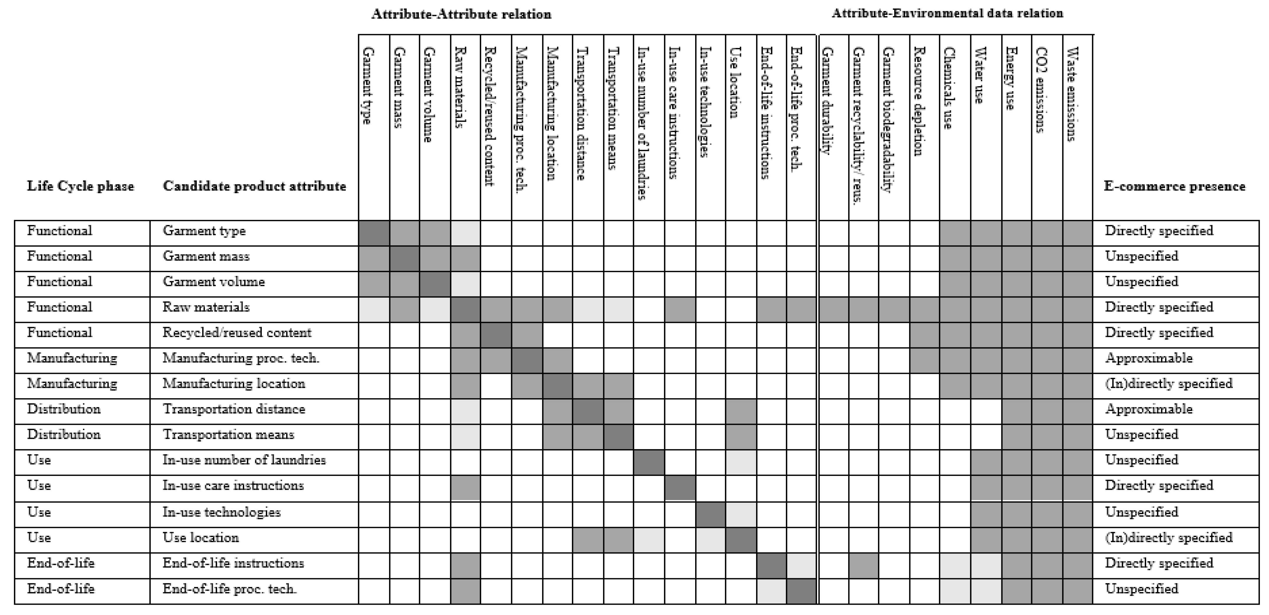
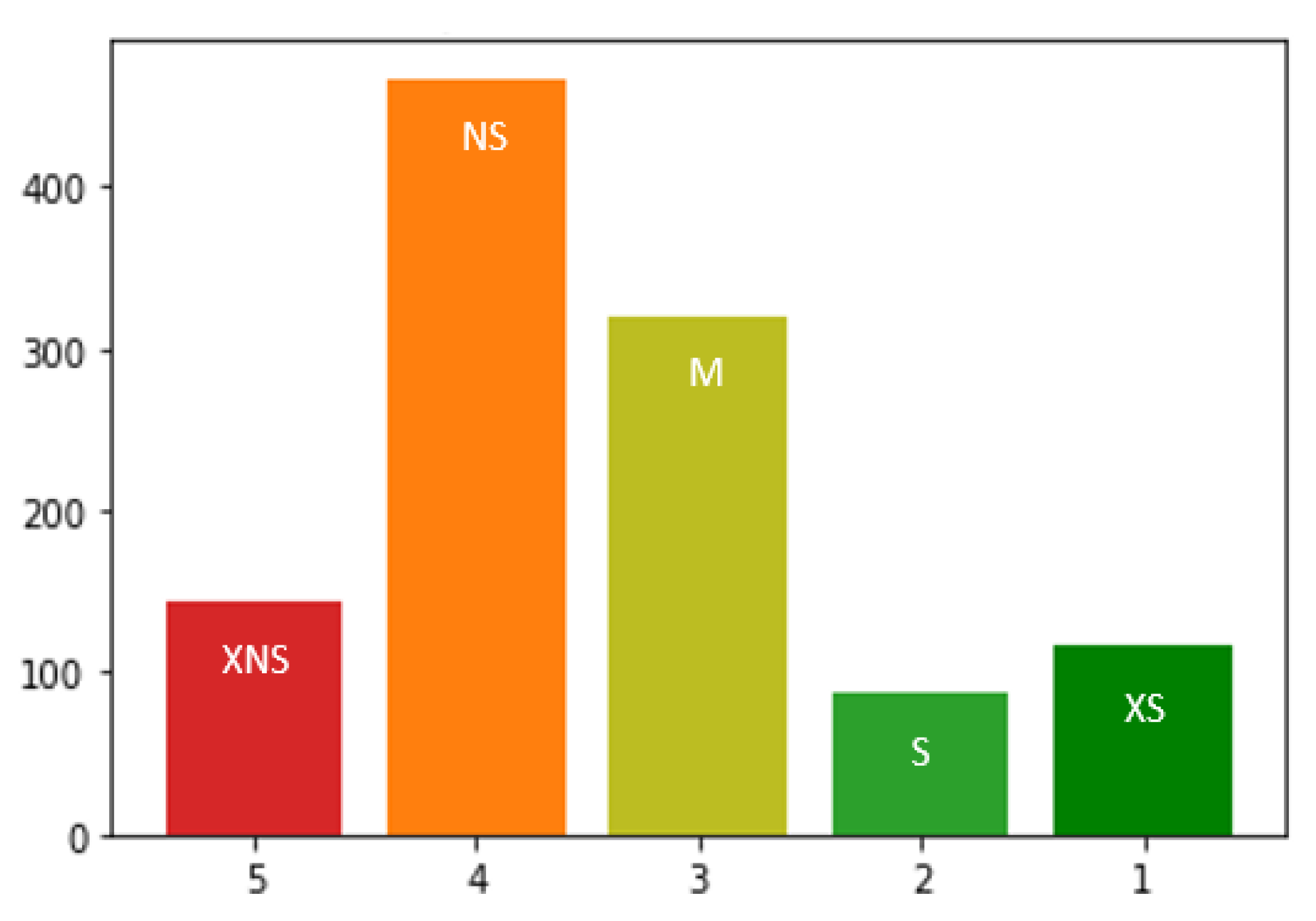
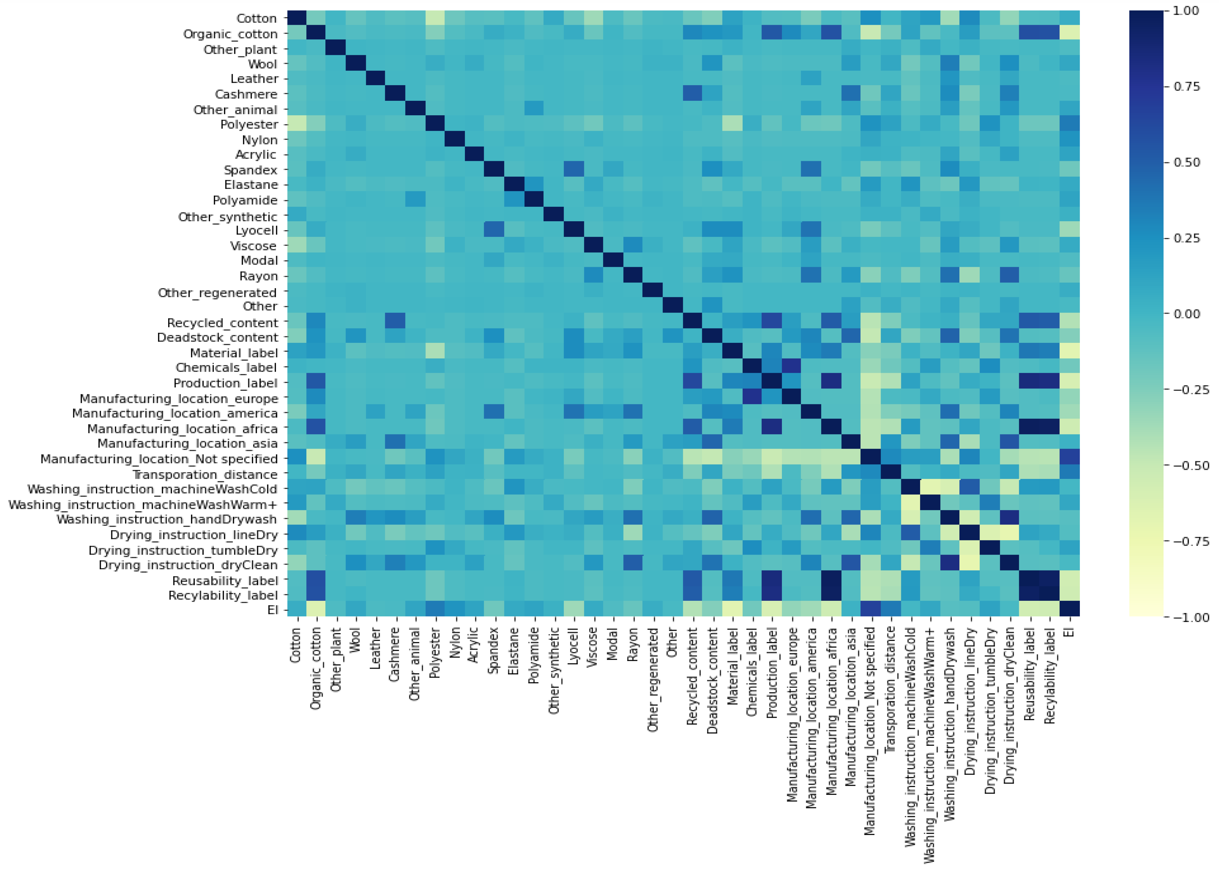
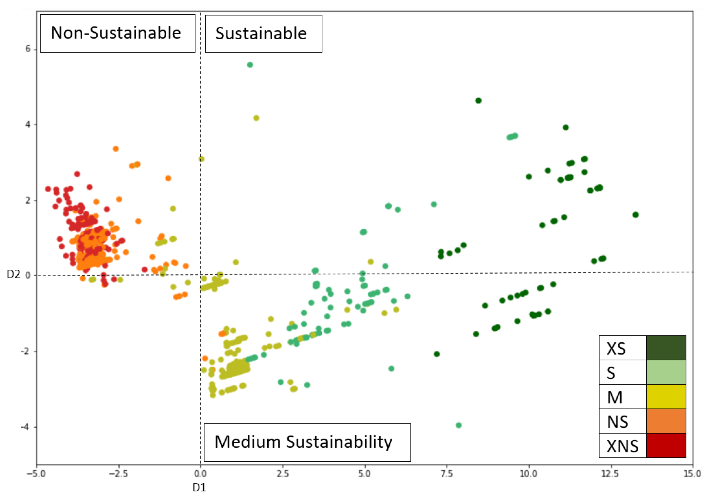
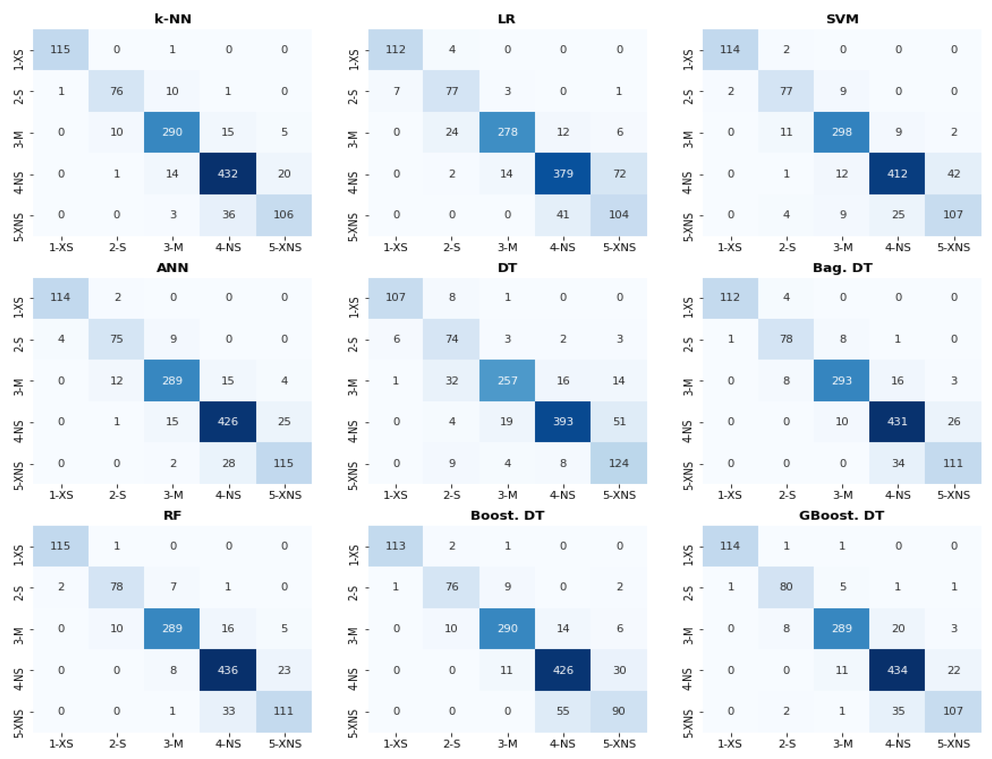
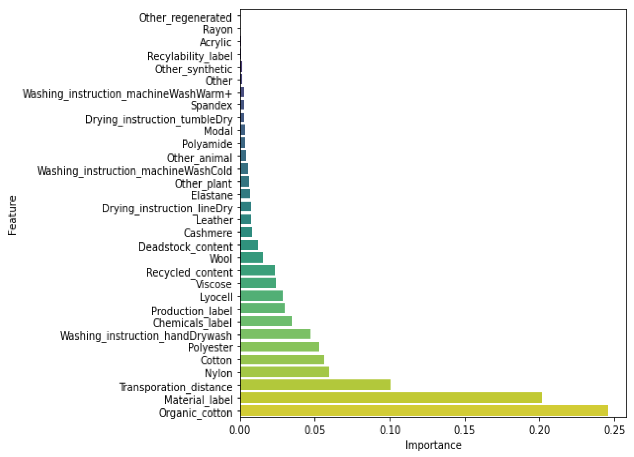
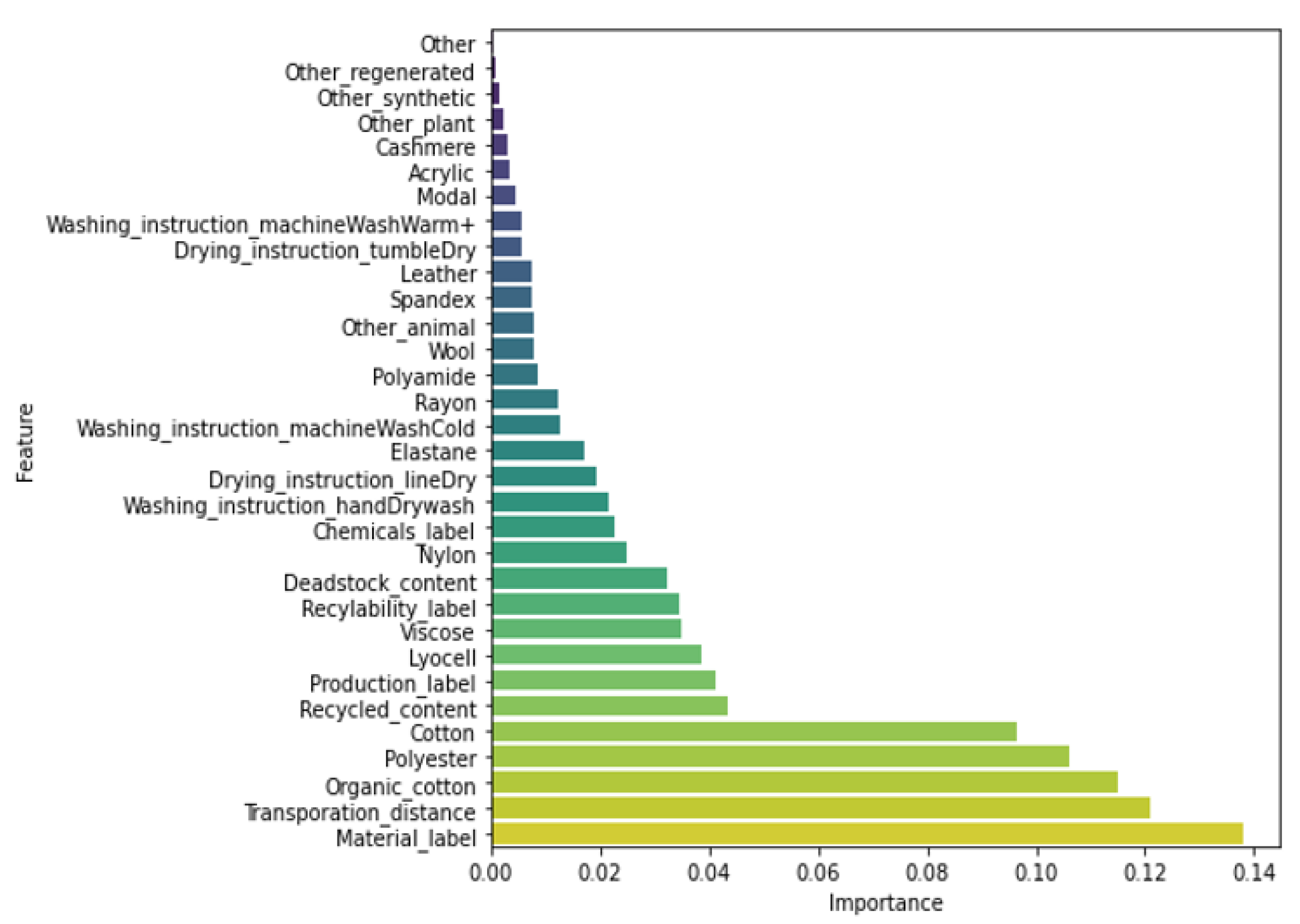
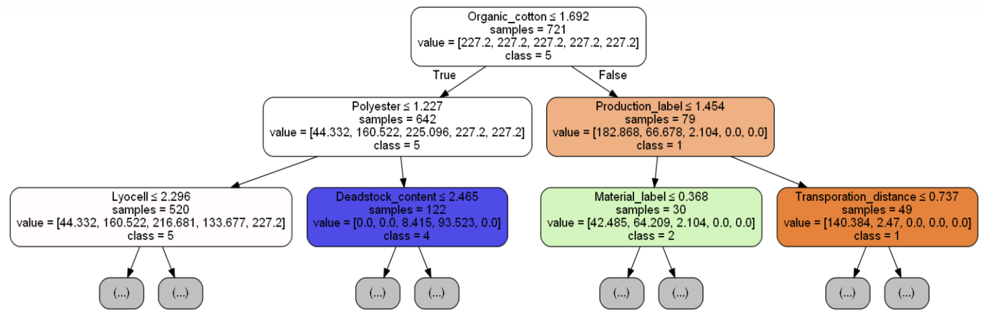
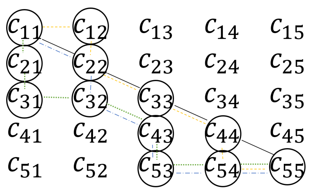
Table 1.
Selected product attributes as features.
| Garment type | Responsibly sourced material label | Approximative transport distance from manufacturer to user | In-use washing instruction |
| % Raw material X 1 | Special production technology label | In-use drying instruction | |
| % Recycled content | Controlled chemicals use label | Recyclable-friendly label | |
| % Reused content | Manufacturing location | Use location | Reusable-friendly label |
1 Percentage of a certain raw material X, with possible values for X being: cotton, organic cotton, flax/linen, jute,
hemp, other plant fibers, silk, wool, leather, camel, cashmere, alpaca, other animal fibers, polyester, nylon, acrylic, spandex, elastane, polyamide, other synthetic fibers, lyocell, viscose, acetate, modal, rayon, other regenerated fibers, other fibers (e.g., fiber mix, metal, etc.).
Table 2.
Classification labels with required single score.
| (5) XNS | (4) NS | (3) M | (2) S | (1) XS |
|---|---|---|---|---|
| [0.00–0.35) | [0.35–0.40) | [0.40–0.50) | [0.50–0.65) | [0.65–1.00] |
Table 3.
The nine machine learning algorithms with the values tested for their hyperparameters.
| Algorithm | Hyperparameter | Values Tested |
|---|---|---|
| k-NN | Number of neighbors to consider (k) | 2, 3, 4, 5, 6, 7, 8, 9 |
| LR | Total penalty strength (λ) | 1, 2, 5, 11, 24, 51, 107, 226, 476, 1000 |
| Strength of each penalty term (α) | 0.0, 0.1, 0.2, 0.3, 0.4, 0.5, 0.6, 0.7, 0.8, 0.9, 1.0 | |
| SVM | Strength of the error term (C) | 1, 2, 5, 11, 24, 51, 107, 226, 476, 1000 |
| Kernel type | linear, polynomial, radial basis function, sigmoid | |
| Kernel gamma | 0.01, 0.06, 0.32, 1.78, 10 | |
| ANN | Number of neurons in the hidden layer (H) | 1, 11, 21 |
| Activation function of the neurons in the hidden layer | sigmoid, rectified linear unit, hyperbolic tangent | |
| Initial learning rate | 0.001, 0.01, 0.1 | |
| Batch size | 1, 10, 100 | |
| Number of epochs | 10, 100 | |
| DT | Minimum number of samples per leaf | 10, 20, 30, 40, 50, 60, 70, 80, 90 |
| Bag. DT | Number of trees | 1, 11, 21, 31, 41, 51, 61, 71, 81, 91 |
| RF | Number of trees | 1, 11, 21, 31, 41, 51, 61, 71, 81, 91 |
| Boost. DT | Number of trees | 1, 11, 21, 31, 41, 51, 61, 71, 81, 91 |
| GBoost. DT | Number of trees | 1, 11, 21, 31, 41, 51, 61, 71, 81, 91 |
| Minimum number of samples per leaf | 10, 20, 30, 40, 50, 60, 70, 80, 90 | |
| Learning rate | 0.01, 0.1, 0.3 |
Table 4.
Average accuracy, recall, precision (with standard deviation), and MSE, Kendall’s Tau-b, OCI of the 9 algorithms and 2 dummy classifiers (The best results for each measure are in bold).
Table 4.
Average accuracy, recall, precision (with standard deviation), and MSE, Kendall’s Tau-b, OCI of the 9 algorithms and 2 dummy classifiers (The best results for each measure are in bold).
| Algorithm | Accuracy Average | Accuracy Std. Dev. | Weighted Recall Average | Weighted Recall Std. Dev. | Weighted Precision Average | Weighted Precision Std. Dev. | MSE | Tau-b | OCI |
|---|---|---|---|---|---|---|---|---|---|
| k-NN | 0.89 | 0.03 | 0.89 | 0.03 | 0.89 | 0.03 | 0.13 | 0.91 | 0.16 |
| LR | 0.84 | 0.02 | 0.84 | 0.02 | 0.85 | 0.01 | 0.19 | 0.87 | 0.22 |
| SVM | 0.89 | 0.02 | 0.89 | 0.02 | 0.89 | 0.02 | 0.17 | 0.89 | 0.17 |
| ANN | 0.90 | 0.01 | 0.90 | 0.01 | 0.90 | 0.01 | 0.12 | 0.91 | 0.15 |
| DT | 0.84 | 0.03 | 0.84 | 0.03 | 0.87 | 0.02 | 0.31 | 0.83 | 0.24 |
| Bag. DT | 0.90 | 0.03 | 0.90 | 0.03 | 0.90 | 0.02 | 0.11 | 0.92 | 0.14 |
| RF | 0.91 | 0.01 | 0.91 | 0.01 | 0.91 | 0.01 | 0.11 | 0.92 | 0.14 |
| Boost. DT | 0.88 | 0.03 | 0.88 | 0.03 | 0.87 | 0.03 | 0.16 | 0.89 | 0.18 |
| GBoost. DT | 0.9 0 | 0.02 | 0.90 | 0.02 | 0.90 | 0.01 | 0.14 | 0.91 | 0.15 |
| Dummy1 | 0.25 | 0.02 | 0.25 | 0.02 | 0.26 | 0.02 | 2.67 | −0.03 | 0.84 |
| Dummy2 | 0.41 | 0.00 | 0.41 | 0.00 | 0.17 | 0.00 | 1.64 | - | 0.63 |
Table 5.
Comparison of the nine machine learning algorithms based on their performance, classification errors, decision rules, and computational complexity. “−” indicates the worst algorithms, “×” the neutral ones and “+” the best of all, for each column.
Table 5.
Comparison of the nine machine learning algorithms based on their performance, classification errors, decision rules, and computational complexity. “−” indicates the worst algorithms, “×” the neutral ones and “+” the best of all, for each column.
| Algorithm | Accuracy Avg. | Accuracy Std. Dev. | MSE | Tau-b | OCI | Classif. Error Types | Decision Rules | Run-Time | Train-Time | Online Learning |
|---|---|---|---|---|---|---|---|---|---|---|
| k-NN | × | − | + | + | + | × | × | − | + | + |
| LR | − | × | × | × | − | × | × | + | × | + |
| SVM | × | × | × | × | × | − | × | + | − | + |
| ANN | + | + | + | + | + | × | × | × | − | + |
| DT | − | − | − | − | − | − | − | + | + | − |
| Bag. DT | + | − | + | + | + | + | × | × | + | × |
| RF | + | + | + | + | + | + | + | × | + | × |
| Boost. DT | × | − | × | × | × | + | + | × | × | + |
| GBoost. DT | + | × | × | + | + | × | × | × | × | + |
Publisher’s Note: MDPI stays neutral with regard to jurisdictional claims in published maps and institutional affiliations. |
© 2022 by the authors. Licensee MDPI, Basel, Switzerland. This article is an open access article distributed under the terms and conditions of the Creative Commons Attribution (CC BY) license (https://creativecommons.org/licenses/by/4.0/).
Share and Cite
MDPI and ACS Style
Satinet, C.; Fouss, F. A Supervised Machine Learning Classification Framework for Clothing Products’ Sustainability. Sustainability 2022, 14, 1334. https://doi.org/10.3390/su14031334
AMA Style
Satinet C, Fouss F. A Supervised Machine Learning Classification Framework for Clothing Products’ Sustainability. Sustainability. 2022; 14(3):1334. https://doi.org/10.3390/su14031334
Chicago/Turabian StyleSatinet, Chloe, and François Fouss. 2022. "A Supervised Machine Learning Classification Framework for Clothing Products’ Sustainability" Sustainability 14, no. 3: 1334. https://doi.org/10.3390/su14031334
Note that from the first issue of 2016, this journal uses article numbers instead of page numbers. See further details here.