
Estimating Future Costs of Emerging Wave Energy Technologies
by
 , , , , and
Pablo Ruiz-Minguela
1,2,* ,
,
Donald R. Noble
3,
Vincenzo Nava
1 ,
,
Shona Pennock
3,
Jesus M. Blanco
1,2 and
and
Henry Jeffrey
3 1
TECNALIA, Basque Research and Technology Alliance (BRTA), Astondo Bidea, Edificio 700, 48160 Derio, Spain
2
School of Engineering, University of the Basque Country, Plaza Ingeniero Torres Quevedo, 1, 48013 Bilbao, Spain
3
Institute for Energy Systems, School of Engineering, The University of Edinburgh, Edinburgh EH9 3FB, UK
*
Author to whom correspondence should be addressed.
Sustainability 2023, 15(1), 215; https://doi.org/10.3390/su15010215
Submission received: 22 November 2022
/
Revised: 14 December 2022
/
Accepted: 15 December 2022
/
Published: 23 December 2022
(This article belongs to the Special Issue Ocean and Hydropower)
Abstract
:The development of new renewable energy technologies is generally perceived as a critical factor in the fight against climate change. However, significant difficulties arise when estimating the future performance and costs of nascent technologies such as wave energy. Robust methods to estimate the commercial costs that emerging technologies may reach in the future are needed to inform decision-making. The aim of this paper is to increase the clarity, consistency, and utility of future cost estimates for emerging wave energy technologies. It proposes a novel three-step method: (1) using a combination of existing bottom-up and top-down approaches to derive the current cost breakdown; (2) assigning uncertainty ranges, depending on the estimation reliability then used, to derive the first-of-a-kind cost of the commercial technology; and (3) applying component-based learning rates to produce the LCOE of a mature technology using the upper bound from (2) to account for optimism bias. This novel method counters the human propensity toward over-optimism. Compared with state-of-the-art direct estimation approaches, it provides a tool that can be used to explore uncertainties and focus attention on the accuracy of cost estimates and potential learning from the early stage of technology development. Moreover, this approach delivers useful information to identify remaining technology challenges, concentrate innovation efforts, and collect evidence through testing activities.
1. Introduction
According to Rubin [1], a technology can be defined as emerging if is not yet deployed or ready for purchase on a commercial scale. The design details of an emerging technology are still preliminary or incomplete, performance has not been sufficiently validated, and it may require new components and subsystems that are not available off-the-shelf. Its current stage of development may range from concept to single device demonstration. On a technology readiness level (TRL) scale [2], emerging technologies encompass a TRL of 2 to 7, which is usually the main focus of research and development programmes. This is the case for wave energy technologies, which are still at the validation phase, or TRL 5 [3].
A common evaluation criterion to assess the feasibility and competitiveness of emerging renewable technologies is the future cost of the commercial-scale version once the technology is mature and widely deployed. The affordability metric typically used is the levelized cost of energy (LCOE) [4]. The LCOE provides a complete picture of technology development in the market by accounting for all lifetime costs and energy production. However, this is not a simple task for prototype technologies due to a lack of previous experience and various uncertainties and unknows. In fact, the direct quantification of the LCOE for single prototypes yields unsuitable results, and therefore a future projection is needed. The LCOE estimate thus represents the future commercial cost that the emerging technology could achieve with sufficient replication provided its technical performance goals are met. The aim of such estimation is twofold: to allow comparison with other technologies currently exploited in the market and to benchmark different cost reduction targets or alternative technology concepts.
The estimation of future costs of wave energy has attracted great interest in order to demonstrate the potential of this renewable energy technology. Various studies have been published providing projections for the entire sector. The OES Technology Collaboration Programme by the IEA developed a study of the international levelized cost of energy for ocean energies in 2015 [5], which directly questioned developers on current costs and future targets. The estimations were updated in 2020 following the same methodology. Although the full report is not accessible, public results show that wave technologies will be able to reach the cost targets defined in the European Strategic Energy Technology Plan (SET-Plan) [6]. These targets are EUR 150/MWh by 2030 and EUR 100/MWh by 2035 for wave energy.
The Joint Research Centre (JRC) periodically publishes ocean energy status reports with cost estimations [3]. Cost are mainly based on the energy technology reference indicator (ETRI) projections for 2010–2050 [7] and the scenario-based cost trajectories to 2050 [8]. These in turn are derived from open literature (both primary and secondary sources), expert judgements, information from other similar technologies, and the application of learning curves with the cumulative capacity foreseen. The higher and lower cost estimates vary significantly due to a lack of a dominating technology and the associated uncertainties related to unproven technologies. Nonetheless, the limited data available from technologies currently under development suggest an LCOE in line or below the SET-Plan targets by 2030 in good resource sites after 1 GW installed capacity [3].
In the UK in 2018, ORE Catapult analysed the cost reduction pathway for wave energy [9]. Single devices reported a cost in excess of GBP 300/MWh together with key cost reductions to GBP 100/MWh after 1GW of deployment through learning by doing, process optimisation, engineering validation, and improved commercial terms. However, again, the lack of data, particularly energy generation, made it hard to accurately estimate the future cost of energy.
Although these studies provide a helpful tool to track the progress of the wave energy sector, they cannot be used to benchmark alternative technology options or assist in decision-making during the different stages of technology development. In this respect, various approaches have been recently proposed to assess wave energy technologies at early stages of development.
The detailed bottom-up techno-economic approach is the most common costing method used for energy technologies. Some future LCOE projections found for wave energy technologies are Oscilla Power’s Triton [10], M3 Wave [11], UGEN [12], or Sandia’s Reference Model Project [13]. In this approach, the design of the wave energy device and balance of plant and array layout, together with the corresponding technical and operational performance parameters, are specified. Based on this information, the capital expenditure (CAPEX) and operational expenditure (OPEX) costs are estimated for a particular deployment site. This cost is then aggregated with other costs such as project development, insurance, and decommissioning costs, and, as a result, an LCOE is obtained. However, this direct method of estimating the future cost of a commercial-scale technology is only suitable for technologies that are close to commercialisation and whose design is well defined. Experience demonstrates that cost estimates for emerging technologies tend to be rather optimistic and significantly lower than the actual cost of the first commercial plant deployed [14]. As the design is further detailed and unforeseen technological issues uncovered in the development process, the estimated costs of these technologies tend to escalate. Subsequently, the relatively high cost of early deployments declines as the technology is replicated and learning is capitalised through more efficient designs and processes.
Alternatively, Têtu [15] proposed a top-down approach based on the target LCOE for the specific market and a technology-agnostic breakdown of costs to derive thresholds for the different cost centres. Various ranges of uncertainties are suggested per development stage as described in [16]. Developers can use this approach internally to inform their technical decisions, but the method lacks transparency where the cost estimation and the allocation of different levels of uncertainty to the detailed breakdown are concerned. A similar approach based on a reverse cost calculation was developed by Pennock [17] for emerging technologies. In this case, the current cost thresholds for early-stage devices are calculated in order to reach the 2030 SET-Plan levelised cost targets [6]. Component-based learning curves are applied, and the resultant breakdown of costs is compared with cost estimates for current devices to identify areas where further cost reduction is still needed. This method provides more clarity but still requires the external assumption of a standard breakdown of costs for the particular class of device (e.g., point absorber), which might differ for the wave energy concept considered. Moreover, uncertainties in the initial estimations are not embedded, but only a sensitivity to the learning rates applied.
To overcome the limitations of the previous methods, this paper proposes a combination of both the bottom-up and top-down approaches. Starting from the current breakdown of costs, uncertainty ranges are assigned depending on the reliability of the estimation and used to derive the first-of-a-kind cost of the commercial technology. Component-based learning rates are then applied to produce the LCOE of a mature technology after achieving installation of a certain capacity through various commercial projects. Learning rates are also subjected to varying uncertainty.
This paper provides a transparent method for estimating of the future costs of wave energy technologies at early stages of development that counters the propensity toward over-optimism. It supplements the IEA-OES international evaluation framework [18], which prescribes the LCOE as the highest-level affordability metric but fails to provide the specific procedures to perform such an estimation. This novel approach is illustrated with the assistance of a case study. The Reference Model Project [13] provides the underlying information to implement this approach. Future LCOE estimations will be compared with direct methods and overall estimations based on expert judgements.
The proposed method is mainly intended for wave energy technology developers. The ultimate goal is to assist them in reducing the high development cost, time, and risk of wave energy technologies. This is quite relevant since there are 87 active wave energy developers, 60% of which are still in the early phases of technology development [19].
2. Methodology
As explained before, the direct quantification of the LCOE is highly unsuitable for prototype technologies. The affordability assessment of an emerging technology requires the future projection of costs with regard to the commercial technology and a first-of-a-kind commercial deployment. To be precise, this farm project should be the smallest size of a wave energy array for the LCOE to yield a meaningful value.
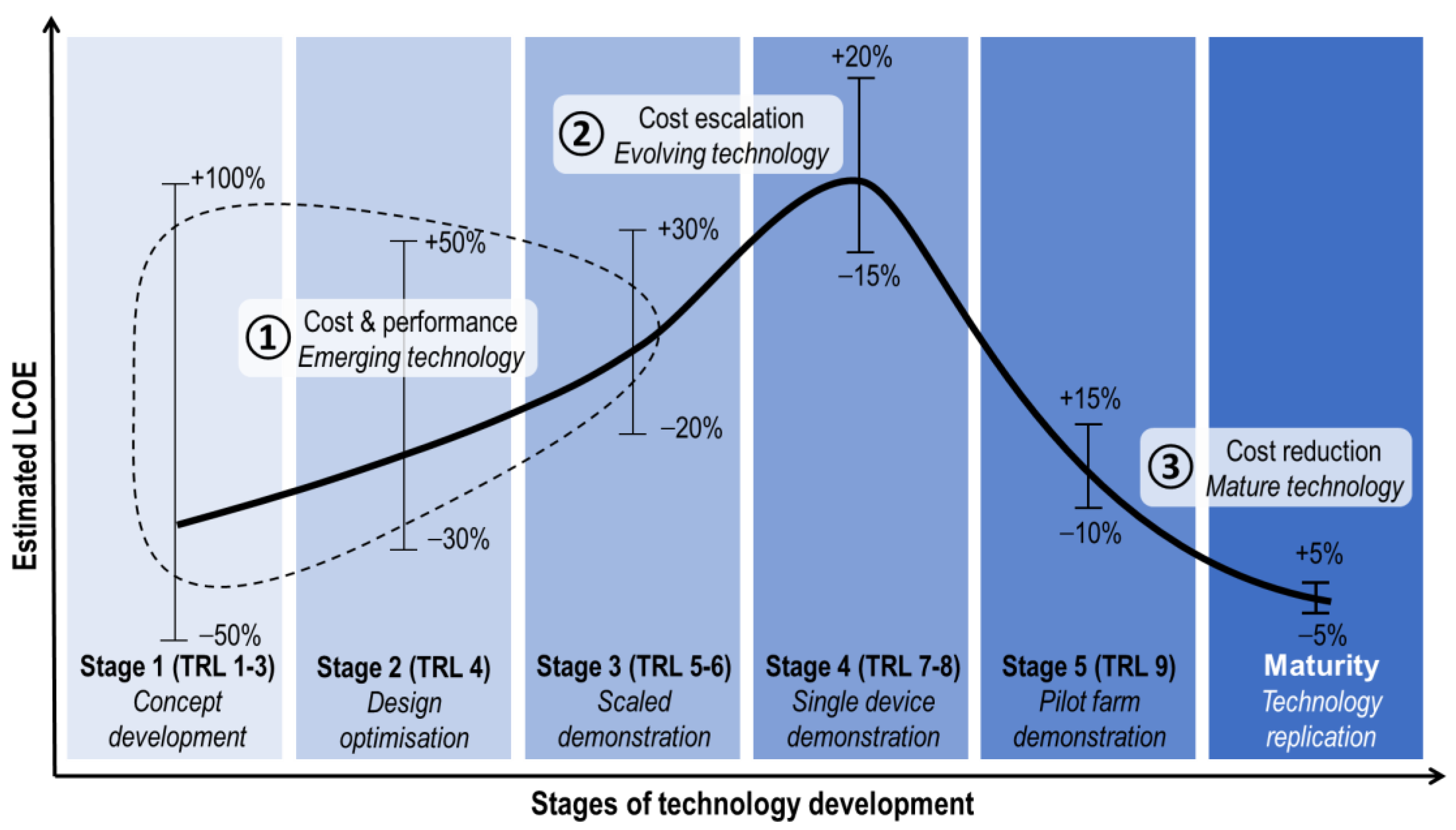
The proposed approach for estimating future costs of emerging wave energy technologies is an indirect method which consists of three main steps as shown in Figure 1:
- Step 1: Estimation of current cost and performance based on a standardised cost and performance breakdown. The emerging technology is assessed with reference to a first-of-a-kind commercial deployment.
- Step 2: Cost escalation to account for uncertainties in the estimations. Uncertainty ranges (lower and upper bounds) are assigned based on the reliability of the input data at each stage of development. Incorporation of standardised contingencies allows for the estimation of costs for the evolving technology with regard to the same first-of-a-kind commercial deployment.
- Step 3: Projection of the future cost based on technology replication. Component-based learning rates are then applied to the upper bound obtained in the previous step. The upper bound is used to counterbalance the inherent optimism bias in early-stage estimates. The technology is assessed in its mature format and when it has been widely deployed.
The reader should note that the stages of technology development are not drawn in a time scale in Figure 1. In fact, time is not evenly distributed through the development stages. More time and effort should be allocated to the initial stages, and the overall development time depends on the selected development trajectory [20].
2.1. Step 1: Estimation of Current Cost and Performance
The first step of this approach involves the bottom-up estimation of the LCOE for the emerging technology at its current state of development. Wave energy technology is decomposed into major cost centres. For emerging technologies which are at lower TRLs, this can include a simplified list of subsystems and cost centres. Further granularity (more breakdown levels) can be added as the technology moves up the TRL scale. Parametric modelling is used to identify functional relationships between physical and performance characteristics of an item and its costs, derived from experience and engineering judgement [21].
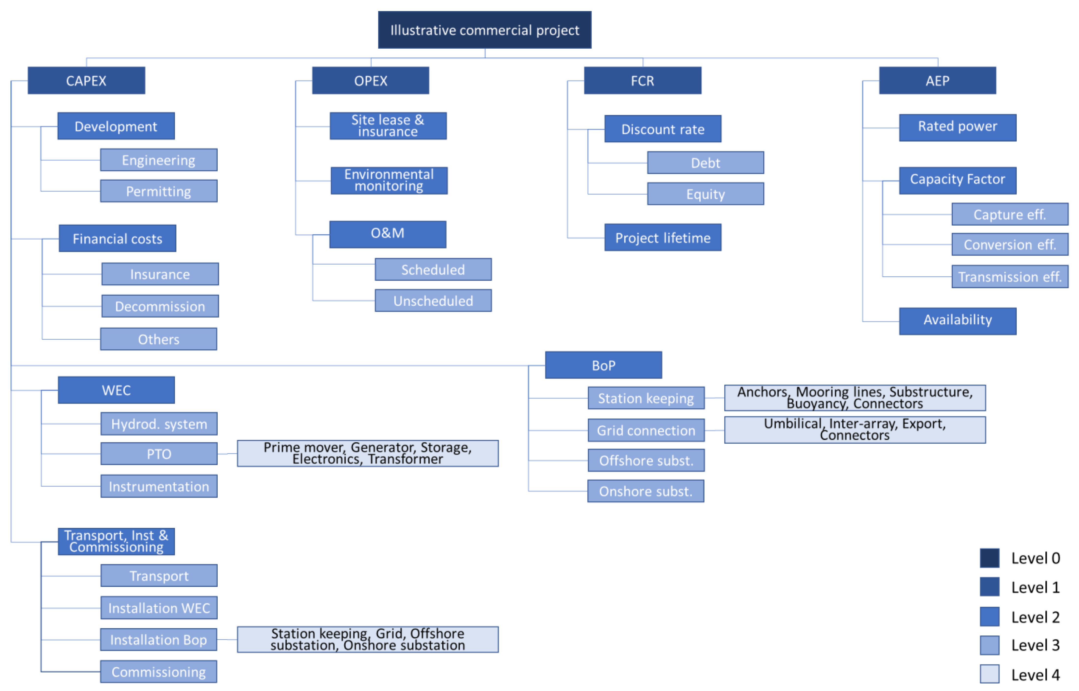
The standardised cost and performance breakdown used in this work is shown in Figure 2 to the fourth level of detail. It builds upon several published guidance documents and tools such as the US Department of Energy reporting guidance [22], BVGA ocean energy value chain study [23], the COE Calculation Tool commissioned by the Danish Transmission System Operator [24], or the DTOceanPlus design tools [25]. These guidance documents are useful to avoid omitting any relevant cost centre.
For the estimation of future costs, a wave energy farm model is created representing an illustrative first commercial project of 50 units. Considering that rated capacity for utility-scale wave energy technologies usually ranges 200–1500 kW [26], this means between 10 and 75 MW in total. The array size lies in the range of the capacity used for cost estimation of commercial farms [27]. The wave farm model should describe deployment site characteristics, water depth, distance to the shore, and other design parameters used.
The first breakdown level fully aligns with the general LCOE equation. Due to the emerging nature of this technology, it is assumed that the annual O&M costs and annual energy production will remain constant during its lifetime. This is a common hypothesis in most techno-economic models and is reasonable provided the long-term average system uptime and site resource are used for the calculation of energy. In this case, the simplified LCOE can be represented using the following expression [28]:
where
- CAPEX, capital expenditure, represents all capital costs associated with the farm development, manufacturing, installation, and decommissioning at the end of the project’s life.
- FCR, fixed charge rate, is the annual return, that is the fraction of the CAPEX needed to meet investor revenue requirements,
- OPEX, annual operating expenditures, include all routine maintenance, operations, and monitoring activity,
- AEP, annual energy production, represents the average net annual energy generated (after accounting for availability) and delivered to the grid.
A brief description of this breakdown is provided in the sections below.
2.1.1. CAPEX
CAPEX can be broken down into farm development costs, financial costs, and all the expenditures associated with the manufacture, installation, and commissioning of both the wave energy converters (WEC) and the balance of plant (BoP).
Development costs comprise engineering (e.g., project management, design engineering, planning, and certification) and permitting services (e.g., environmental studies, consenting, and licenses). Financial costs include insurance during construction and decommissioning bonds.
The generic WEC system breakdown [29] has been used to structure the costs of WEC and BoP manufacture. The WEC contains:
- A hydrodynamic system, comprising structural elements, ballast, and ancillary systems (e.g., navigation lights, bollards, and deck crane).
- Power take-off (PTO), including the prime mover (either mechanical, pneumatic, hydraulic, or direct drive), electrical generator, short-term storage, and power electronics.
- Instrumentation, control, and safety systems, ranging from sensors, comms, control software, cooling, lubrication, firefighting, and back-up power.
On the other hand, the BoP includes all the supporting infrastructure and auxiliary systems of the wave farm needed to deliver the energy other than the WEC itself [30], i.e.:
- Station-keeping, including the foundation (e.g., anchors and piles), mooring lines for compliant systems, or substructure for rigid systems.
- Grid connection, comprising the umbilical, intra-array, and export power cables.
- Offshore substation and switchgear.
The installation and commissioning cost of the WEC and the different subsystems comprising the BoP are considered.
A basic estimate of some of these costs, such as development and financial costs, can be expressed as a percentage of total CAPEX costs. Guidance can be found in [31], where Têtu and Fernandez Chozas performed a comprehensive literature review in order to build a cost database for wave energy projects. However, as we will see in Section 2.2, whenever feasible, it is much better to use more sophisticated techno-economic methods to increase the accuracy of the cost estimations.
2.1.2. OPEX
OPEX is usually measured on an annual basis. These costs can be broken down into operation and maintenance (O&M) costs, as well as site leases and insurance during operation. Costs related to site leases and insurance are self-evident. Insurance transfers the risks associated with the replacement of faulty components during the underwritten period of time (usually 5 years).
O&M costs include servicing of the WECs and BoP. Depending on the ability to plan the activities, these costs can be split between:
- Scheduled maintenance, which includes periodic inspections and preventive actions.
- Unscheduled maintenance, which comprises all corrective actions to restore the operational capabilities of the farm and the logistical cost of waiting for a suitable weather window.
Again, when data is scarce, OPEX can be estimated as a percentage of CAPEX [31]. This is a basic estimate with high uncertainty. As the technology developer starts designing operational plans, techno-economic estimations based on the failure rate of components and subsystems, vessel cost, operation time, and the cost of spares should be a more appropriate tool to improve the accuracy.
2.1.3. Financial Assumptions
A key consideration for utility-scale renewable energy technologies is the impact of the availability and cost of capital on LCOE values. The discount rate (a proxy of the cost of capital) and the project lifetime are the two main parameters.
Assumptions of discount rates are crucial for the assessment of wave energy technology and investment decisions. However, they are subject to a significant degree of uncertainty since the expectations and risk perceptions of investors and project sponsors differ significantly. Discount rates are often estimated based on the weighted average cost of capital (WACC) [32]. The WACC gives an estimate of the cost of raising capital, which is equivalent to the approximate return required by potential creditors (debt) and investors (equity).
The simplified LCOE expression uses the fixed charge rate (FCR) [33]:
where is the discount rate and is the project lifetime in years.
2.1.4. AEP
Calculating net AEP should closely follow the IEC’s technical specification 62600-100, “Electricity producing wave energy converters—Power performance assessment” [34]. Assumptions regarding the wave energy resource at the intended deployment site and the numerical method for estimating performance should be documented and justified. Particularly, the estimations should account for losses due to directionality, shallow water, and array interaction effects, together with WEC ancillary energy consumption needs.
The AEP is the product of the rated power of the array, the capacity factor, and the availability
where:
- 8766 is the average total hours in a year.
- P is the rated power of the farm.
- CF is the capacity factor.
- AF is the availability factor.
CF represents the ratio of the energy produced by the technology continuously operating over a year compared to the energy that could have been produced at the rated power during the same period. In turn, CF can be computed as the product of the device capture efficiency (i.e., the ratio of absorbed and rated power), the conversion efficiency (i.e., the ratio of converted and absorbed power), and the transmission-to-grid efficiency (i.e., the ratio of grid and device output power).
AF is the fraction of time in a year that the wave energy technology is capable of producing energy [35]. By convention, the zero production periods (i.e., wave resources lie below or above certain limits) are counted against the CF but not against the AF.
2.2. Step 2: Cost Escalation to Account for Uncertainties
For commercial technologies, the costs of a farm project are commonly calculated based on quotes or published data, and when costs are not readily available, they can be estimated using engineering handbooks and numerical models. However, for emerging technologies that have not yet been built at a commercial scale, the direct estimation method might be misleading due to the associated uncertainty in making the cost appraisals. The importance of estimating initial costs is paramount since it will determine the total additional spending required for an emerging technology to be cost competitive in the market.
Actually, LCOE estimates of wave energy technologies can vary widely across studies depending on the external properties and the complexity of the analysis methods utilized [21]. Both aspects were highlighted in the previous step. For a correct interpretation of results, it is essential to undertake a careful examination of the underlying assumptions of farm size, deployment site characteristics, cost of capital, materials, and service vessels.
The current step of the method deals with a third source of variability, namely the uncertainty of the input data for the wave energy farm model. Assigning a range with a nominal confidence band is a good practice that provides much more useful information for decision-making. However, emerging technologies imply that little experience is available to assign ranges of uncertainty to costs.
Several strategies can be used to allocate expected ranges of accuracy to the estimations based on expert judgement. Previsic [16] assigns uncertainty ranges as a double function of the stage of technology development and the source of input data for the estimation for wave energy technologies. Hence, estimation accuracy may vary from −30% to +80% for simplified estimations and technologies at the concept stage and from −5% to +5% for detailed estimates of mature technologies. Fernandez-Chozas [24] applies Previsic’s uncertainty ranges to the AEP data for each development stage and source of performance estimates (i.e., power matrix and standard sea states). Likewise, organisations including EPRI [36], the DOE [37], and the Association for the Advancement of Cost Engineering International (AACE) [38] have defined several cost estimate classes ranging from “simplified” to “finalised”. Parsons performed an exhaustive review and comparison of cost contingency practices and standards to conclude that AACE represents best industry practices [39]. Cost estimation should require increasing levels of effort (and expense) as the technology moves from concept and preliminary design to demonstration and replication.
The ability to properly combine uncertainties from different cost factors is crucial. The individual estimates and their uncertainties can be combined statistically provided they can be calculated with statistical techniques. Rothwell [40] shows that the current engineering guidelines are consistent with contingencies equal to the standard deviation of the cost estimate. He derives the standard deviation from an 80% confidence level using a lognormal probability distribution, since most cost estimate accuracy ranges are non-symmetric. This is because final costs are usually higher than those estimated, and there is no probability that the final cost will ever be less than zero (which is a possibility with the normal distribution).
Table 1 presents the suggested contingencies and expected accuracy ranges used by current engineering guidelines for the different types of cost estimates as well as the corresponding lognormal property fit of the uncertainty ranges. Statistical properties have been normalised by the mode, the most likely estimate. The median represents the 50% probability, which is an indication of the basic uncertainty factor. The standard deviation (Std) has been adjusted with reference to the upper bound in AACE guidelines for an 80% confidence level interval. It can be noted that the statistical fit results in a Std within the range of the expected accuracy values except for the final estimate, in which it is slightly lower.
Assuming independence of each factor, the probability distributions can now be combined. This is particularly simple if each distribution can be treated as lognormal. In such instances, the final distribution is also lognormal, with the logarithmic standard deviation given by the square root of the sum of squares of the individual geometric standard deviations. Moreover, the error propagation technique can be used to combine uncertainties from multiple variables in the techno-economic expressions of the wave energy LCOE model.
Propagation of error (or uncertainty) is a calculus-derived statistical calculation designed to combine uncertainties from multiple quantities to another quantity. It is based on a set of simple mathematical rules. The standard deviations are used to calculate the resulting uncertainty. Furthermore, provided variables are independent, covariances will be avoided. The general formula for error propagation is given by:
where q is a function that depends on the estimated quantities, x, …, z and their associated uncertainties, δx, …, δz.
The process for error propagation involves:
- Identifying the uncertain variables in the techno-economic expression for cost estimation.
- Taking partial derivatives with respect to each of the variables identified in the previous step.
- Multiplying the partial derivatives by the associated uncertainty to calculate the error contribution from each variable.
- Adding the contributions in quadrature.
The uncertainty estimation in the LCOE is not direct, but it is calculated by means of its formula involving CAPEX, OPEX, FCR, and AEP. In turn, each of these factors were derived in Step 1 using basic parametric relationships. Error propagation is used to calculate the aggregated uncertainty in a cascading manner from the lowest level of the standard cost and performance breakdown. For instance, the structural cost of the hydrodynamic system can be calculated from three techno-economic variables: the unit cost of the main raw material (EUR/kg), a coefficient to account for the manufacturing complexity (-), and the structural weight (kg). Ranges of uncertainty in the material unit cost (exogenous factor), maturity of manufacturing processes (suppliers’ capability), and estimation of the structural weight (design accuracy) will determine the aggregated uncertainty in the estimation of the hydrodynamic system cost, in this case, the geometric mean of the standard deviations. This estimate in turn will be combined with other capital expenditures to derive the uncertainty in the WEC, farm CAPEX, and finally the LCOE.
2.3. Step 3: Projection of the Future Cost with Technology Replication
The third and final step of the methodology involves the application of learning curves to project the future costs of wave energy technology once it has been sufficiently replicated and the estimation of uncertainties in the forecast due to learning. Different learning mechanisms have been described in the literature, such as in [41,42,43]. The most important mechanism is technological learning. Other learning factors may include:
- Economic learning, i.e., shifting production to low-wage countries.
- Social learning; as stakeholders become more familiar, they increase trust in one another.
- Financial learning; as banks and investors gain confidence in a new technology, they reduce the expected interest rates.
These exogenous factors have a significant impact on the LCOE estimation, but unfortunately, they can only be accounted for within the initial assumptions or through sensitivity analysis.
Technological learning is an endogenous factor that encompasses learning by research in the early stages due to R&D investments, learning by doing during the production stage due to higher efficiency of manufacturing processes, learning by using in the initial stage of introduction of the technology into the market, and learning by interaction in the diffusion of the technology incidentally reinforcing the previous factors. Scale effects are also part of the technological learning mechanism, both upsizing (i.e., the increase in rate power) through technology redesign leading to lower unit costs, and economies of scale (i.e., mass production) through standardisation allowing upscaling of production facilities.
The analysis presented in this paper uses the learning curve method as the most applied approach. The commonly used formulation originates from empirical observations across diverse energy technologies that often evidence a log-linear relationship between cost reductions driven by manufacturing, standardisation, scale of production and use, and cumulative installed capacity or production [44]. In the simplest form, it can be expressed as:
where Y is the cost of the technology and x represents the cumulative experience (often characterised by the installed capacity in MW). The constants a and b denote the cost of the first commercial deployment and the rate of cost reduction, respectively. Note that b represents the slope in a log-log scale in Equation (5). The cost reduction associated with duplication of experience is referred to as the learning rate (LR).
The independent variable x in Equation (5) reflects all the factors that influence the cost trajectory of the technology. Often, combinations of technological learning occur at each stage, and their contributions may change during the development of a technology over time. Furthermore, single-factor learning curves do not necessarily describe the underlying factors of cost reduction [44]. Some components and subsystems in wave energy farms, such as electrical infrastructure and offshore operations, are not entirely new to the market. They build on the experience gained from more mature sectors, a disaggregated approach that can account for individual learning effects at the component level leading to improved cost reduction estimations for emerging technologies which lack historical data. This can take advantage of past learning rates for direct comparable technologies in order to build a composite learning rate. In addition, it can break apart the impact of raw material spending (an exogenous parameter) from other cost reductions due to cumulative experience.
Learning rates found in the literature for wave energy technologies mainly rely on expert judgements, expectations, and assumptions. They tend to differ widely even at the subsystem level [8]. Overall LRs range from a low 9% [45] to an optimistic 30% [5]. Component-based learning rates range 1% to 12% [27]. Similarly, SI Ocean [46] included a learning rate of 3% for the capacity factor in its LCOE projections.
Since there is little empirical evidence to establish the learning rates for WEC technologies, the component-based learning approach used in this work allocates them depending on the stage of development of the individual components. Three main categories are defined:
- Mature components. These are technologies already established in the market that have well-known characteristics and limited potential for cost reduction due to learning. Low learning rates of 0–5%. E.g., export power cables.
- Evolving components. These have niche market commercialisation and have the potential for significant cost reductions due to learning. Medium learning rates of 5–10%. E.g., prime mover.
- Emerging components. These have not been commercialised yet, but their potential learning cost reductions are high. High learning rates of 10–20%. E.g., maintenance operations.
The upper bound of learning rates is consistent with analyses such as the PelaStar cost of energy [47] and WaveBoost [48]. In these studies, the technological maturity of each major cost item is categorised as “mature”, “emerging”, or “nascent/emerging 2” with 5%, 10%, and 15–20% learning rates, respectively. The lower bound refer to more conservative analyses such as NEMS [49]. Technologies classified as “conventional”, “evolutionary”, and “revolutionary” are assigned 1%, 5%, and 10% learning rates, correlatively.
Assigning error margins to LRs is recommended to avoid overrepresentation in cost reduction estimates [50]. Forecasts are highly sensitive to uncertainties in the progress ratio. As in the previous step, the error can be calculated from the error propagation theory [43]:
where δb is the uncertainty in the experience parameter and δLR is the resulting uncertainty.
Moreover, the cost reduction for a technology cannot be realised continually. There will be a bare minimum or baseline cost necessary to build a technology. As suggested in Section 2.2, segregating the price of raw materials from the estimation of manufactured component costs is a recommended strategy to prevent this situation.
3. Case Study and Results
The application of the proposed cost estimation methodology is illustrated with the help of one of the reference models (RMs) for wave energy technologies [13]. The RM project team, led by Sandia National Laboratories (SNL), included a partnership between the US Department of Energy (DOE), the National Renewable Energy Laboratory (NREL), and other US laboratories. The RMs provide a non-proprietary, open-source instrument for technical and economic assessment and validation of design tools, as well as the identification of cost reduction pathways and research priorities to meet the affordability targets. The wave energy models [51] reproduce three common archetypes, namely, a point absorber (RM3), an oscillating wave surge converter (RM5), and an oscillating water column (RM6).
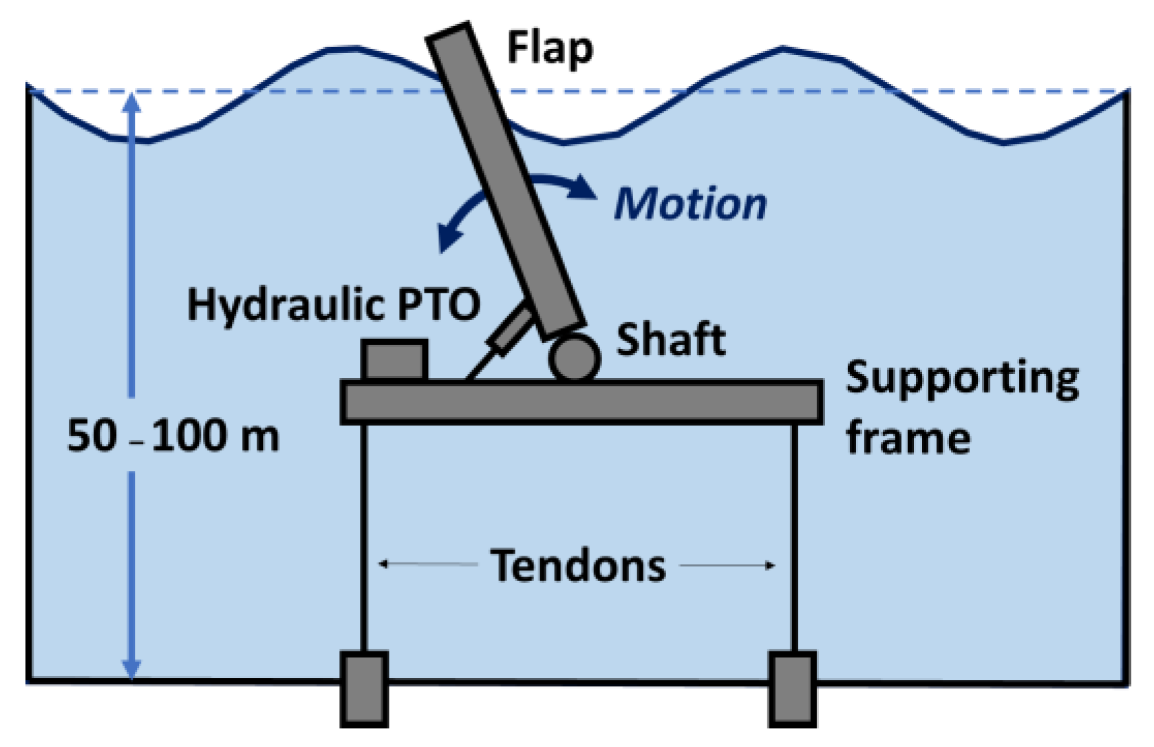
The present case study is based on the RM5, a floating oscillating wave surge converter (OWSC) designed for a wave site near Eureka in Humboldt County, California. The OWSC is one of the most promising wave energy technologies in terms of its energy absorption capabilities [52]. It basically consists of a vertical flap that faces the waves and articulates in its lower part for rotation. The surge motion of waves creates a back-and-forth movement from which energy is extracted [53]. Several OWSC designs have been proposed, including Aquamarine Power’s Oyster [54], AW-Energy’s WaveRoller [55], Resolute Marine’s Wave2O [56], and Langlee’s Robusto [57]. The floating version of OWSCs tackle the potential environmental restrictions of nearshore shallow waters, at the same time opening the way to harness the higher wave energy resource in deep-water sites [58].
Figure 3 shows a schematic of the floating OWSC device. The flap rotates against the supporting frame to convert wave energy into electrical power from the motion induced by incoming waves. An oleo-hydraulic PTO with two rams, high pressure accumulators, electrical generator, and corresponding switchgear is used to transform the oscillation in electrical power. The device is tension-moored to the seabed in deep waters (50 to 100 m) through four tendons.
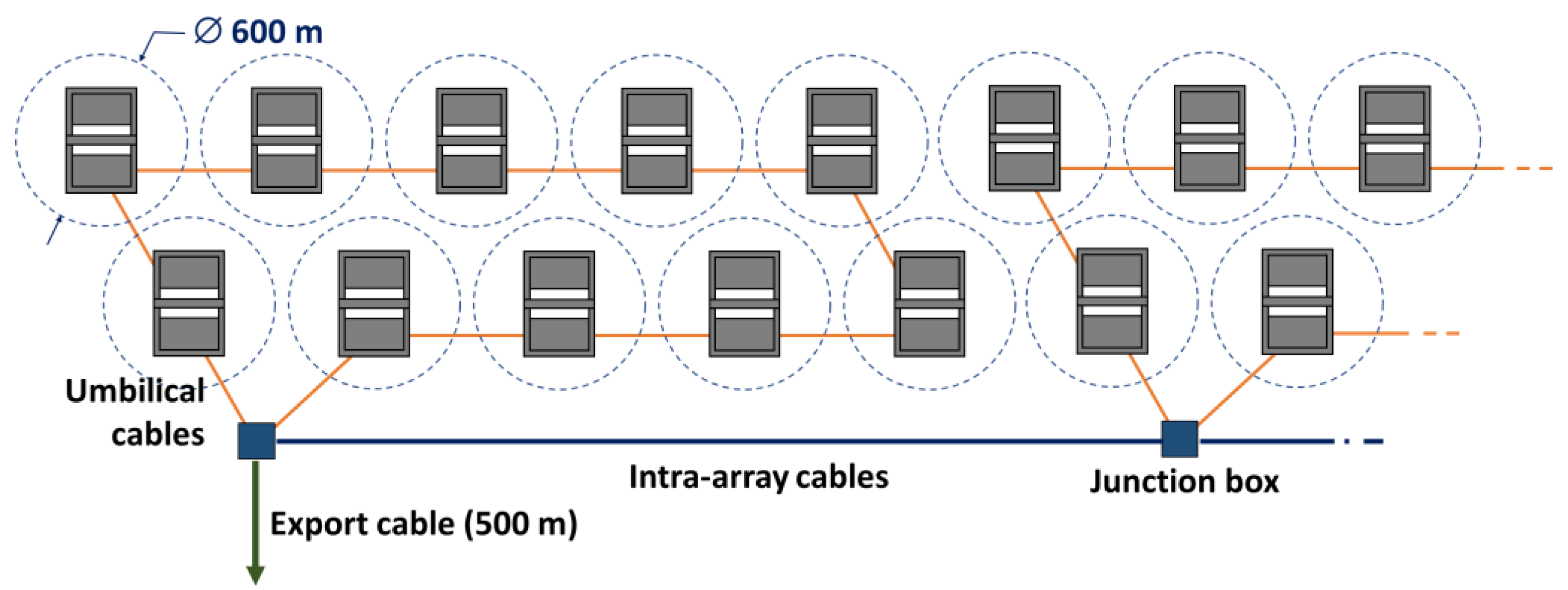
NREL created a techno-economic model for the assessment of the LCOE with multiple scenarios ranging from a single RM5 device to arrays of 10, 50, and 100 units [59]. For the estimation of future costs, this case study uses the cost breakdown of the 50-unit farm model, which can be considered representative of the first commercial project. The RM5 has a rated capacity of 360 kW, which results in an 18 MW wave energy farm.
The array configuration is depicted in Figure 4. A staggered configuration with 600 m spacing between the devices to accommodate moorings is considered to avoid collisions with vessels and produce negligible hydrodynamic losses. Groups of 10 devices are interconnected by umbilical cables as shown in the figure. Electricity is then transmitted to a junction box. Intra-array cables connect the five junction boxes. Lastly, a three-phase AC export cable delivers energy to the shore. Cable landing is accomplished using directional drilling. Close to the deployment site, there is a port with facilities well-suited for installation and maintenance activities and a 60 kV onshore substation.
The key design parameters and main assumptions are included in Table 2. Further details of RM5 design can be found in [58].
3.1. Step 1: Cost and Performance of the 50-Unit Farm
NREL’s model for the 50-unit farm results in an estimated LCOE of USD 0.78/kWh [59]. The proposed method yields a slightly lower estimate (USD 0.72/kWh) due to the 10% contingency in CAPEX costs included in NREL’s model. Contingency is a consequence of the propagation of uncertainties, and consequently it is accounted for in Step 2.
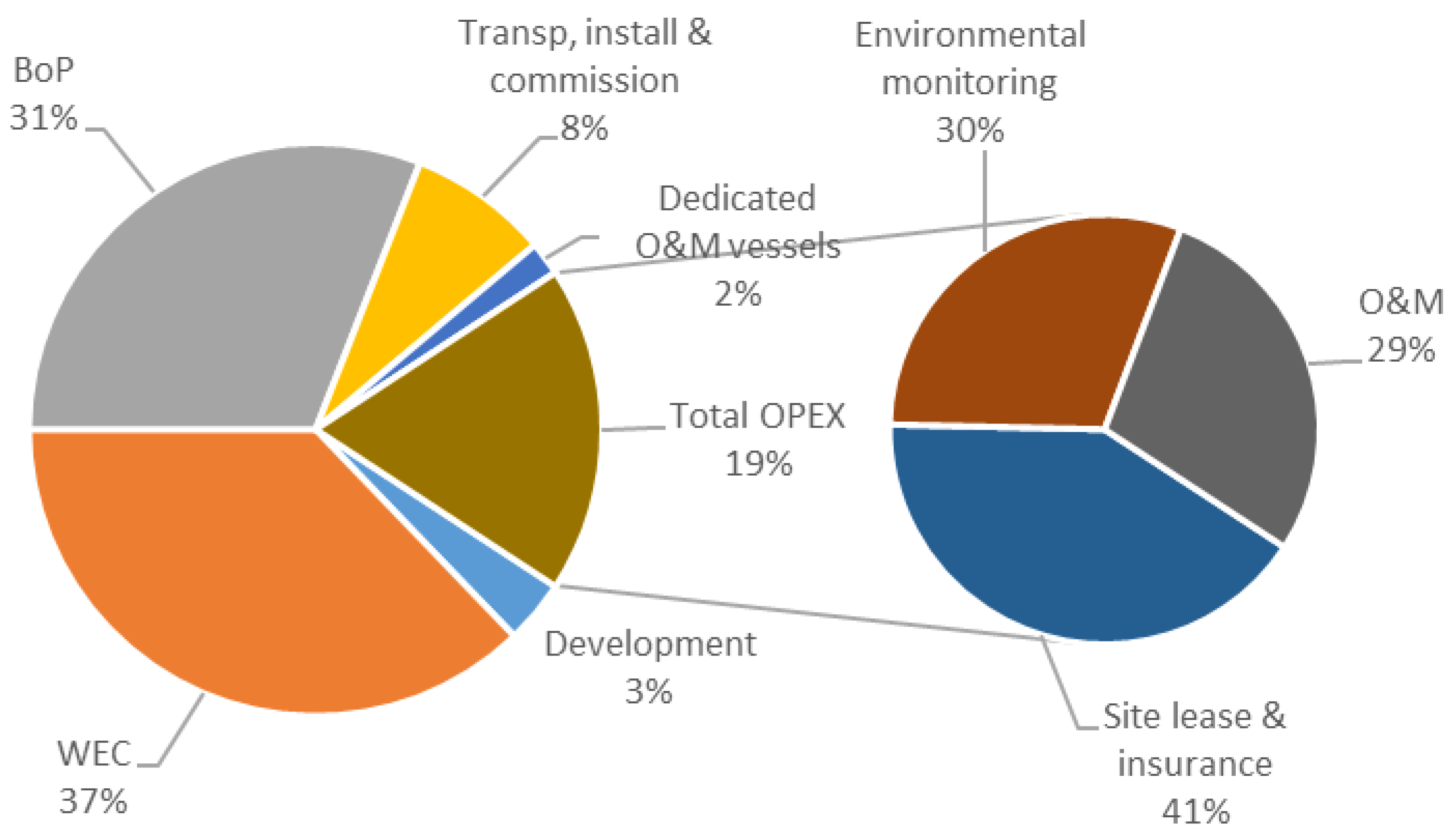
The detailed breakdown of CAPEX and OPEX costs, financial assumptions, and annual energy production taken directly from the RM5 model are presented in Table 3. The last column outlines the modelling basis directly extracted from [59]. The resulting percentage contribution to the lifetime costs of the main cost centres is shown in Figure 5.
3.2. Step 2: Cost Escalation to Account for Uncertainties
The RM5 model has inherent uncertainties regarding performance, design, and economics. NREL carried out a qualitative uncertainty assessment of both design and performance [58]. Levels of uncertainty, from low to very high, were assigned to various components of the model depending on whether this facet was assessed using test/field data (low), modelled data (medium), or engineering judgment (high). Aspects that were not addressed were assigned a “very high” level of uncertainty.
The qualitative assessment has been mapped to the AACE’s uncertainty classes and corresponding quantitative standard deviation (Std). Sometimes “low to medium” and “medium to high” levels of uncertainty were used. In these two cases, an average value between the two adjacent classes is assumed as shown in Table 4. None (0%) is only used whenever the parameter has no implicit uncertainty.
Uncertainty is propagated upwards in the breakdown structure using the generic Equation (4) until a final LCOE is was obtained. The method comprises four specific categories of functions:
- Addition of several components (applicable to CAPEX and OPEX cost centres). The absolute uncertainty is the geometric mean of individual absolute uncertainties.
- Multiplication or division of several components (applicable to AEP). The relative uncertainty is the geometric mean of the individual relative uncertainties.
- Financial uncertainty with a variable discount rate (d) and constant lifetime (n) and differentiation of the FCR with respect to the discount rate.
- Uncertainty in LCOE. A sequential combination of multiplication (CAPEX × FCR), addition (OPEX), and division (AEP) computed with the help of Equations (8) and (9).
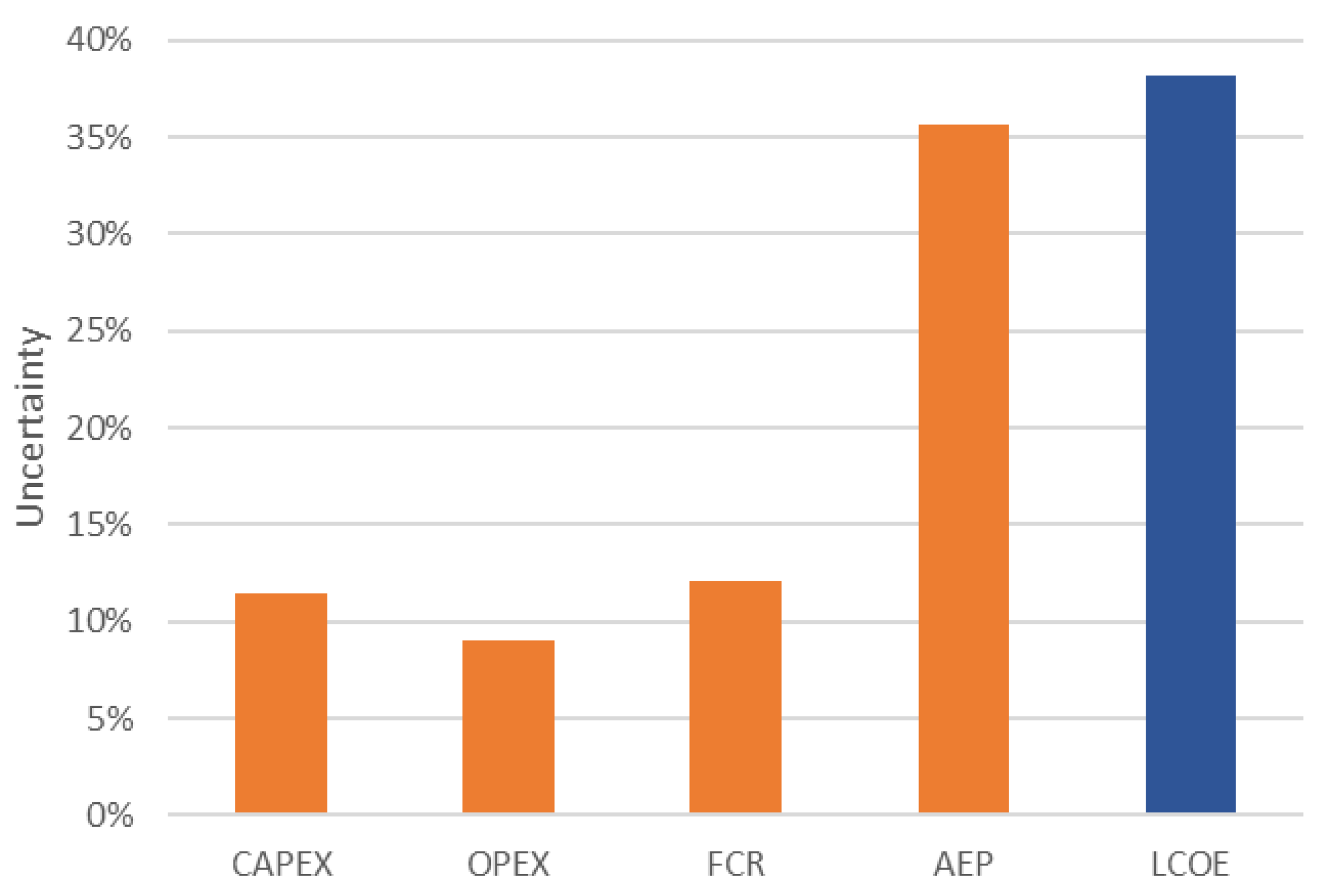
The detailed results are presented in Table 5. Following this procedure, the LCOE results in an upper and lower bound of USD 1.33/kWh and USD 0.50/kWh, respectively. The Std of the LCOE uncertainty is 38.2%, which gives an indication of the contingency to be considered. It can be noticed that the AEP is the greatest contributor to the global uncertainty. The rest of the components in the LCOE (Equation (1)) are slightly above 10%, which fairly matches the aforementioned assumption of contingency in the NREL’s model. Figure 6 displays the resulting uncertainties for the high-level components in the LCOE equation. It is also worth mentioning that the NREL’s model estimates USD 1.44/kWh for a small array of 10 units [59].
3.3. Step 3: Projecting the Future Cost of the Mature Technology
The last step of the methodology involves the optimisation of the current version of the technology through learning by doing and economies of scale (endogenous factors) leading to cost reduction. Learning is proportional to the installed capacity, having impact on the CAPEX, OPEX, and to a certain extent on the AEP. Component-based learning rates are applied to the upper bound obtained in the previous step. In this case study, LCOE results are projected once 1 GW of the emerging technology has been deployed. Selection of 1 GW installed capacity allows comparison with JRC forecasts [3]. The NREL’s model provides component-based learning rates for the PTO. For other cost centres, they only provide a qualitative indication depending the predicted innovation potential [58]. A baseline cost has also been included marking a hard threshold beyond which no more learning would be possible. This baseline is based on the 100-unit model, which corresponds to a fully commercial project.
The component-based learning rates are classified in three main categories according to the technology type as shown in Table 6. Learning rates of mature technologies are matched with low uncertainty, whereas evolving and emerging technologies are assumed to have medium and high uncertainties, respectively. The same standard deviations as in Table 4 are used.
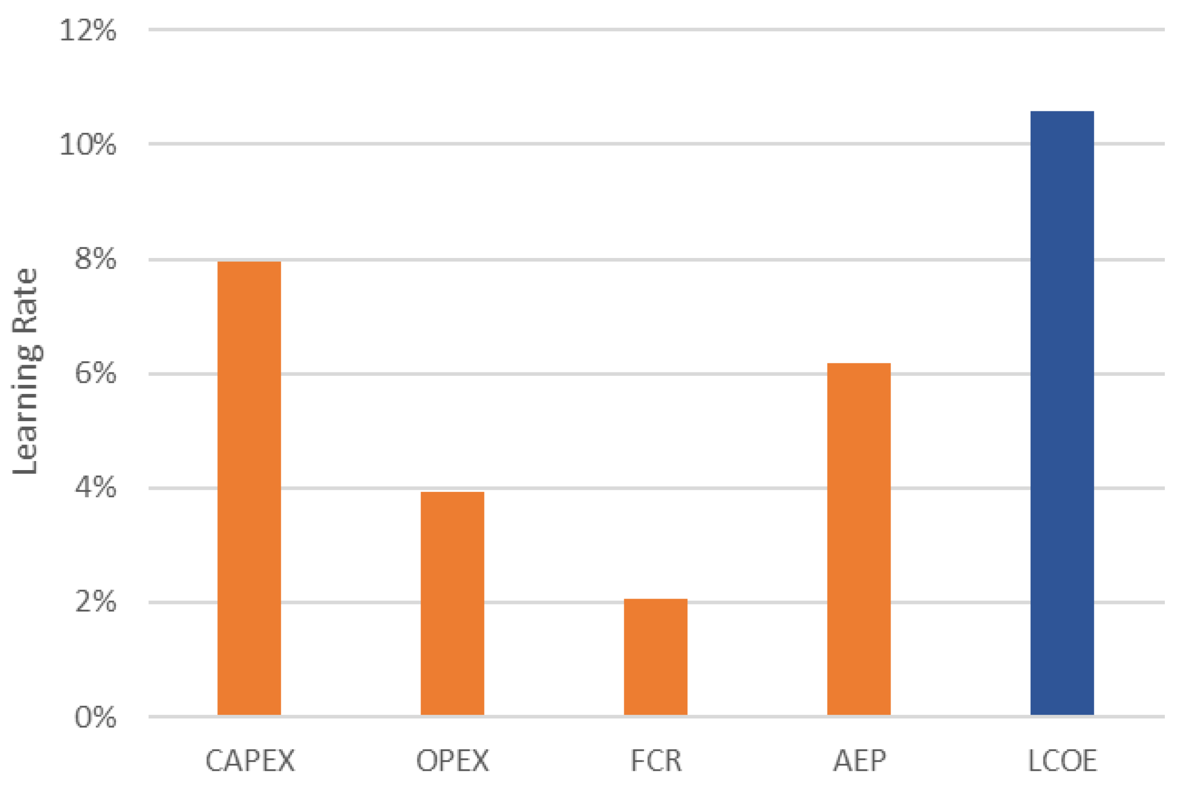
Detailed results are shown in Table 7. Component-based projections are combined using the same basis as in Table 3 to derive the corresponding LRs at the immediate upper level. This process is repeated until the aggregated LR, 10.6%, is finally obtained. Figure 7 displays the resulting LR for the high-level components in the LCOE equation. The proposed method estimates the future cost of energy at USD 0.69/kWh. The baseline cost suggested is USD 0.62/kWh, which is higher than the lower bound of USD 0.50/kWh identified in Step 2. Finally, the NREL’s 100-unit model results in exactly the same estimate of USD 0.69/kWh [59].
4. Discussion
The implementation of this novel method for estimating costs of the RM5 WEC leads to an initial LCOE (Step 1) for this emerging technology of USD 0.72/kWh. The application of uncertainties (Step 2) shows that the LCOE could be as high as USD 1.33/kWh in its first commercial deployment. Finally, the projection of future costs using component-based learning rates (Step 3) forecasts that LCOE could be reduced to USD 0.69/kWh after 1 GW of cumulative capacity has been deployed (USD 0.60–0.83/kWh accounting for uncertainties in the learning rate). These results follow the cost progress pattern of a wave energy technology along the development stages depicted in Figure 1. Moreover, results align with the NREL’s direct estimation method for 50-unit, 10-unit, and 100-unit farms, respectively. The reader should note that while the NREL’s model envisages a progressive cost reduction with the increase in farm size, the proposed method follows the development cost pattern peaking at an intermediate stage.
Despite the significant cost reduction that can be achieved through learning, the projection of future commercial costs for the RM5 technology is still far from the SET Plan EUR 0.15/kWh target for 2030, since the starting cost for this emerging technology is well above this target. A closer look at the case study results unveils two main factors for the discouraging result leading to a very high projection of costs.
On the one hand, the AEP is subjected to large uncertainty (35.7%) penalising the LCOE from which learning can start to happen. In fact, the lowest bound in Step 2, USD 0.50/kWh, remains far distant from the SET Plan target for wave technologies. On the other hand, the baseline costs are established for the 100-unit farm which limit the ability to capitalise cost reductions through component-based learning beyond a certain deployment level. This outcome reinforces the recommendation to technology developers of deploying R&D activities aimed at collecting evidence that can reduce uncertainty with regard to the availability factor, capture efficiency, and baseline costs, since they will significantly lower the overall uncertainty in the LCOE and open the way to a starker cost reduction.
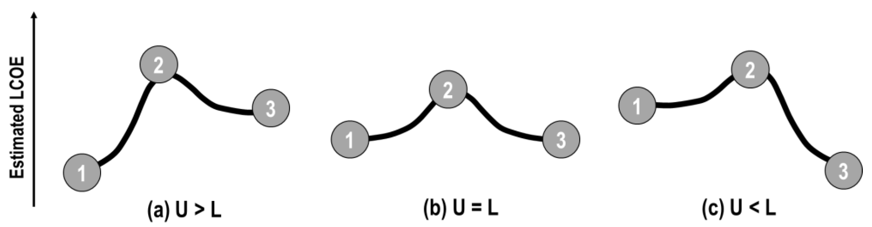
The case study results only illustrate one of the possible trajectories that an emerging technology can experience in connection with the estimation of future costs. The methodology described before can be repeated with several other wave energy archetypes such as reference models RM3 and RM6 [13] leading to potentially dissimilar results. Actually, three scenarios, depicted in Figure 8, can be envisaged through combining different levels of uncertainty (U) and learning capacity (L).
- (a)
- Uncertainty overshadows potential learning (U > L). This trajectory leads to a long-term projection of cost in Step 3 higher than the initial LCOE. The LCOE calculated in Step 1 should be much below the energy price in the addressed market. Otherwise, radical changes must be implemented in the emerging technology. Provided technology development is continued, efforts should be driven to collecting evidence that lowers the cost estimation uncertainty in Step 2. If successful, the LCOE reassessment should lie in either scenario (b) or (c) at the next development stage.
- (b)
- Uncertainties in the same range of learning capacity (U ≈ L). This scenario leads to a similar future projection of costs as the initial LCOE estimation in Step 1. For emerging technologies with a high uncertainty level, such as the RM5, there is still room to fill up the critical cost and performance knowledge gaps. Again, if efforts are successful, the LCOE reassessment at the next development stage should lie in scenario (c). Nevertheless, technologies that combine relatively low levels of uncertainty and learning capacity should exhibit an LCOE in Step 1 below the energy price in the addressed market, or else technology breakthroughs should be implemented to meet the commercial goals.
- (c)
- Learning potential dominates uncertainty (U < L). A higher learning capacity provides a more favourable scenario for the emerging technology. The future projection of costs will be lower than the initial estimation in Step 1. If the long-term estimation in Step 3 is below the energy price in the addressed market, the technology can pass to the next development stage without major changes. However, care must be taken that the emerging technology is not stuck in scenarios (a) or (b) above when a new LCOE assessment is performed.
The affordability of emerging wave energy technologies could be improved thanks to a combined exploitation with other marine-space activities. Shared infrastructure will effectively reduce future cost estimations. The cost centres involved could be either structural elements for fixed devices integrated in breakwaters and existing platforms, or electrical components, if connected to the same onshore grid point. Although this strategy can offset the LCOE, it is worth noting that the global uncertainty of the cost estimation will not be significantly altered since the AEP is the greatest contributor.
The error propagation method proved to be a useful tool to identify the greatest contributors to uncertainty in the standardised breakdown of CAPEX, OPEX, FCR, and AEP. The addition of several components as per Equation (8) decreases the relative uncertainty, which suggests that expanding the breakdown levels in the CAPEX and OPEX is a useful strategy to improve the quality of future LCOE projections. However, the product of components as per Equation (9), such as AEP, will always enlarge the relative uncertainty, which indicates that the emerging technology should strive to enhance the accuracy of the performance estimations and keep to a minimum the number of energy transformation stages in the PTO design.
The statistical fit of lognormal properties with an 80% confidence interval, borrowed from previous research in other engineering applications, led to quantitative results in line with the NREL’s cost model assumptions for the CAPEX. The propagated uncertainty obtained with the proposed method (11.4%) is close to the 10% contingency for the 50-unit RM5 farm assumed by the NREL’s cost model. It matches the AACE’s Class 2 estimate (i.e., detailed estimate, project definition between 30% and 75%). Additionally, the proposed cost estimation method points out other sources of uncertainty in the OPEX and in the financial assumptions, which can carry out similar contingencies (i.e., 9% for OPEX and 12.1% for the FCR), but not considered by the NREL. Furthermore, the overall uncertainty in AEP matches the equivalent of a simplified estimate (Class 4).
Component-based learning rates and baseline costs are also useful to avoid over-optimism. LRs between 2% (mature) and 20% (emerging) were assigned to the standardised breakdown resulting in an aggregated LR of 10.6%. Although the method of quantification is highly qualitative, this indirect estimation helps identify inherent limitations in cost reduction that could be hidden if considered in the LR of the emerging WEC as a whole.
The main merit of this cost estimation method is to provide a transparent and traceable way to assess the future affordability of wave energy technologies under development. It focuses the attention on the accuracy of the cost estimates at an early stage. Instead of oversimplifying the LCOE quantification when there are still many knowledge gaps, the approach includes these unknowns in the form of uncertainties to counter any optimism bias for the first commercial deployment. The method delivers useful information to identify remaining technology challenges, concentrate innovation efforts, and collect evidence through testing activities. The importance of estimating first commercial farm costs is paramount since it impacts the total additional spending required for an emerging technology to be cost competitive in the market and achieve long-term LCOE projection. Starting a cost reduction from an over-optimistic point will ultimately yield highly unrealistic figures of LCOE for mature technology.
The consideration of a first commercial deployment is useful for tracking the evolution of costs in the development cycle of the emerging technology, but it cannot be used to estimate the learning investment or the timescales to achieve future LCOE. The wave energy sector needs to achieve certain deployment level before consistent cost reduction occurs, as the wind industry has shown. This will offset the forecasts by some years and increase the amount of learning investment required to converge to this cost.
This method contains some limitations:
- The statistical treatment of cost centres, and particularly the assumption of independence, will tend to underestimate the overall uncertainty and therefore the resulting LCOE. For instance, the failure rate correlates both the availability and the unscheduled maintenance cost. To counterbalance, this method takes the conservative upper bound of the 80% confidence interval. Alternatively, Monte Carlo methods could be implemented to combine the individual uncertainties, provided the technology developer can build a fully parametric model of the emerging technology.
- Some costs do not scale linearly with the installed capacity, such as grid connection. As the array gets bigger in subsequent projects, the share of grid connection in the LCOE will be reduced. This method considers a constant size of the farm, but economies of scale (larger farms) can be included in the learning rates to account for these situations.
- The uncertainty in learning rates follows the same engineering guidelines as costs due to a lack of previous experience.
- Learning by research, innovation, and upscaling leading to performance and reliability increase is not considered in the future LCOE projection. The cost estimation method can also be used in the next iteration of the technology and the results compared. Note, however, that the innovations introduced in the emerging technology should bring greater benefits than the corresponding uncertainty increase due to lower maturity in order to lead to a more attractive cost projection.
5. Conclusions
This paper presents a novel method to estimate future costs of emerging wave energy technologies that counters the human propensity to over-optimism. Compared with state-of-the-art direct estimation methods, it provides a tool that can be used to explore uncertainties and focus attention on the accuracy of the cost estimates and potential learning from the early stage of technology development. Moreover, this approach delivers useful information to identify remaining technology challenges, concentrate innovation efforts, and collect evidence through testing activities.
A case study was used to illustrate this method. Results show that the uncertainties are in the same range of potential future learning, leading to a future projection of costs similar to the initial LCOE estimation. Technology development efforts should be driven to fill the critical cost and performance knowledge gaps.
The quantitative results are very specific to this case study. Actually, three possible cost trajectories have been discussed in this paper, depending on how the learning potential of the emerging technology weights against the inherent uncertainties. The most favourable scenario is when the learning potential of the emerging technology dominates the inherent uncertainties, and hence the technology can pass to the next development stage without major changes.
While this method has been demonstrated for wave energy technologies, the approach is fully transferrable to any nascent electricity generation technology without any loss of generality.
Future work could apply this approach to a state-of-the-art wave device which is currently undergoing full-scale demonstration, as well as improve the quantification of component-based learning rates and the propagation of corresponding uncertainties. Complementary to this research stream, further work could also pinpoint promising innovation strategies to overcome the challenges that have been identified through this approach.
Author Contributions
Conceptualization and writing—original draft, P.R.-M.; methodology, P.R.-M., D.R.N. and S.P.; review and editing, D.R.N., V.N., S.P. and J.M.B.; visualization, P.R.-M. and D.R.N.; funding acquisition, J.M.B.; resources and supervision, H.J. All authors have read and agreed to the published version of the manuscript.
Funding
This research received no external funding.
Institutional Review Board Statement
Not applicable.
Informed Consent Statement
Not applicable.
Data Availability Statement
Not applicable.
Acknowledgments
The authors would like to thank the Basque Government through the support of the research group IT-1514-22.
Conflicts of Interest
The authors declare no conflict of interest. The funders had no role in the design of the study; in the collection, analyses, or interpretation of data; in the writing of the manuscript; or in the decision to publish the results.
Abbreviations
The following abbreviations are used in this manuscript:
| AEP | Annual Energy Production |
| AF | Availability Factor |
| BoP | Balance of Plant |
| CAPEX | CAPital EXpenditure |
| CF | Capacity Factor |
| D | Discount rate |
| FCR | Fixed Charge Rate |
| LCOE | Levelized Cost of Energy |
| LR | Learning Rate |
| N | Project lifetime |
| O&M | Operation and Maintenance |
| OPEX | OPerational EXpenditure |
| OWSC | Oscillating Wave Surge Converter |
| P | Rated power |
| PR | Progress Ratio |
| PTO | Power Take-Off |
| RM | Reference Model |
| TRL | Technology Readiness Level |
| WACC | Weighted Average Cost of Capital |
| WEC | Wave Energy Converter |
References
- Rubin, E.S. Evaluating the Cost of Emerging Technologies; Carnegie Mellon: Oslo, Norway, 2016. [Google Scholar]
- De Rose, A.; Buna, M.; Strazza, C.; Olivieri, N.; Stevens, T.; Peeters, L.; Tawil-Jamault, D. Technology Readiness Level: Guidance Principles for Renewable Energy Technologies; European Commission: Petten, The Netherlands, 2017; pp. 17–27. [Google Scholar]
- Magagna, D.; European Commission; Joint Research Centre. Ocean Energy: Technology Development Report; Publication Office of the European Union: Luxembourg, 2020; ISBN 978-92-76-12428-3. [Google Scholar]
- Mai, T.; Mowers, M.; Eurek, K. Competitiveness Metrics for Electricity System Technologies; National Renewable Energy Laboratory: Golder, CO, USA, 2021; p. 1765599. [Google Scholar]
- OES|Cost of Energy. Available online: https://www.ocean-energy-systems.org/oes-projects/levelised-cost-of-energy-assessment-for-wave-tidal-and-otec-at-an-international-level/ (accessed on 29 August 2022).
- Implementation Working Group Ocean Energy. SET-Plan—Ocean Energy Implementation Plan; European Commision: Brussels, Belgium, 2021; p. 51. [Google Scholar]
- Lacal Arantegui, R.; Jaeger-Waldau, A.; Vellei, M.; Sigfusson, B.; Magagna, D.; Jakubcionis, M.; Perez Fortes, M.; Lazarou, S.; Giuntoli, J.; Weidner Ronnefeld, E.; et al. ETRI 2014—Energy Technology Reference Indicator projections for 2010-2050; Publications Office of the European Union: Luxembourg, 2014. [Google Scholar]
- Tsiropoulos, I.; Tarvydas, D.; Zucker, A. Cost Development of Low Carbon Energy Technologies: Scenario-Based Cost Trajectories to 2050, 2017 Edition; Publications Office of the European Union: Luxembourg, 2018. [Google Scholar]
- Smart, G.; Noonan, M. Tidal Stream and Wave Energy Cost Reduction and Industrial Benefit; Offshore Renewabel Energy Catapult: Glasgow, UK, 2018; p. 21. [Google Scholar]
- Mundon, T. Oscilla Power Triton 1310 System Overview and Baseline LCOE Calculations; Marine and Hydrokinetic Data Repository; Oscilla Power, Inc.: Washington, DC, USA, 2022. [Google Scholar]
- Morrow, M. M3 Wave DMP/APEX WEC Projected LCOE. Available online: https://mhkdr.openei.org/submissions/300 (accessed on 29 August 2022).
- Moliner, E.G. Cost Analysis of the UGEN; MSc Dissertation, Instituto Superior Tecnico: Lisboa, Portugal, 2016. [Google Scholar]
- Sandia National Laboratories Reference Model Project (RMP). Available online: https://energy.sandia.gov/programs/renewable-energy/water-power/projects/reference-model-project-rmp/ (accessed on 29 August 2022).
- Simon, R.; Rubin, E.S.; van der Spek, M.; Booras, G.; Berghout, N.; Fout, T.; Garcia, M.; Gardarsdottir, S.; Kuncheekanna, V.N.; Matuszewski, M.; et al. Towards Improved Guidelines for Cost Evaluation of Carbon Capture and Storage; Zenodo. 2021. Available online: https://zenodo.org/record/4643649 (accessed on 14 December 2022).
- Têtu, A.; Fernandez Chozas, J.A. Proposed Guidance for the Economic Assessment of Wave Energy Converters at Early Development Stages. Energies 2021, 14, 4699. [Google Scholar] [CrossRef]
- Previsic, M.; Siddiqui, O.; Bedard, R. EPRI Global E2I Guideline Economic Assessment Methodology for Offshore Wave Power Plants; Electric Power Research Institute: Palo Alto, CA, USA, 2004. [Google Scholar]
- Pennock, S.; Garcia-Teruel, A.; Noble, D.R.; Roberts, O.; de Andres, A.; Cochrane, C.; Jeffrey, H. Deriving Current Cost Requirements from Future Targets: Case Studies for Emerging Offshore Renewable Energy Technologies. Energies 2022, 15, 1732. [Google Scholar] [CrossRef]
- Hodges, J.; Henderson, J.; Ruedy, L.; Soede, M.; Weber, J.; Ruiz-Minguela, P.; Jeffrey, H.; Bannon, E.; Holland, M.; MacIver, R.; et al. An International Evaluation and Guidance Framework for Ocean Energy Technology; IEA-OES: Lisbon, Portugal, 2021. [Google Scholar]
- ELBE European Strategic Cluster Partnership in Blue Energy. Available online: http://www.elbealliance.eu/home (accessed on 14 December 2022).
- Weber, J.; Costello, R.; Nielsen, K.; Roberts, J. Requirements for Realistic and Effective Wave Energy Technology Performance Assessment Criteria and Metrics. In Proceedings of the 13th European Wave and Tidal Energy Conference, Naples, Italy, 1–6 September 2019; p. 10. [Google Scholar]
- Mukora, A.; Winksel, M.; Jeffrey, H.F.; Mueller, M. Learning Curves for Emerging Energy Technologies. Proc. Inst. Civ. Eng. Energy 2009, 162, 151–159. [Google Scholar] [CrossRef]
- LaBonte, A.; O’Connor, P.; Fitzpatrick, C.; Hallett, K.; Li, Y. Standardized Cost and Performance Reporting for Marine and Hydrokinetic Technologies. In Proceedings of the 1st Marine Energy Technology Symposium (METS13), Washington, DC, USA, 10–11 April 2013; pp. 10–11. [Google Scholar]
- BVG Associates. Ocean Power Innovation Network Value Chain Study: Summary Report; BVG Associates: Swindon, UK, 2019; p. 26. [Google Scholar]
- Chozas, J.F.; Kofoed, J.P.; Jensen, N.E.H. User Guide—COE Calculation Tool for Wave Energy Converters: Ver. 1.6—April 2014; Department of Civil Engineering, Aalborg University: Aalborg, Denmark, 2014. [Google Scholar]
- DTOceanPlus DTOceanPlus—Advanced Design Tools for Ocean Energy Systems Innovation, Development and Deployment. Available online: https://www.dtoceanplus.eu/ (accessed on 29 August 2022).
- OceanSET. OceanSET Third Annual Report; European Commission: Brussels, Belgium, 2022; p. 89. [Google Scholar]
- Carbon Trust. Accelerating Marine Energy: The Potential for Cost Reduction—Insights from the Carbon Trust Marine Energy Accelerator; Carbon Trust: London, UK, 2011; p. 64. [Google Scholar]
- NREL LCOE Calculator. Available online: https://sam.nrel.gov/financial-models/lcoe-calculator.html (accessed on 14 December 2022).
- Hamedni, B.; Mathieu, C.; Bittencourt Ferreira, C. SDWED Deliverable D5.1 Generic WEC System Breakdown; The Danish Council for Strategic Research: 2014; p. 33. Available online: https://www.sdwed.civil.aau.dk/digitalAssets/97/97538_d5.1.pdf (accessed on 14 December 2022).
- Marques, M.I. Deliverable D8.2 Analysis of the Supply Chain; DTOceanPlus; European Commission: Brussels, Belgium, 2020; p. 78. [Google Scholar]
- Têtu, A.; Fernandez, C. Deliverable D8.1—Cost Database; LiftWEC; European Commision: Brussels, Belgium, 2020. [Google Scholar]
- Innovation Fund. Methodology for Relevant Costs Calculation; InnovFund-LSC-2021; European Commision: Brussels, Belgium, 2022; p. 38. [Google Scholar]
- Previsic, M. Economic Methodology for the Evaluation of Emerging Renewable Technologies; RE Vision Consulting, LLC: Sacramento, CA, USA, 2011; p. 14. [Google Scholar]
- IEC TS 62600-100:2012; Marine Energy—Wave, Tidal and Other Water Current Converters—Part 100: Electricity Producing Wave Energy Converters—Power Performance Assessment. International Electrotechnical Commission: Geneva, Switzerland, 2012; p. 35.
- ISO 14224:2016; Petroleum, Petrochemical and Natural Gas Industries—Collection and Exchange of Reliability and Maintenance Data for Equipment. ISO: Geneva, Switzerland, 2016; p. 178.
- EPRI. Technical Assessment Guide (TAG)—Power Generation and Storage Technology Options; Electric Power Research Institute: Palo ALto, CA, USA, 2013. [Google Scholar]
- DOE. Cost Estimating Guide; U.S. Department of Energy: Washington, DC, USA, 1997; p. 298. [Google Scholar]
- AACE International. Cost Estimate Classification System—As Applied In Engineering, Procurement, and Construction for the Hydropower Industry Tcm Framework: 7.3—Cost Estimating and Budgeting; AACE: Morgantown, WV, USA, 2013; p. 15. [Google Scholar]
- Parsons, E.L. Waste Management Project Contingency Analysis; U.S. Department of Energy, Federal Energy Technology Center: Pittsburgh, PA, USA, 1999; p. 23. [Google Scholar]
- Rothwell, G. Cost Contingency as the Standard Deviation of the Cost Estimate. 2005. Available online: https://www.researchgate.net/profile/Geoffrey-Rothwell/publication/237635336_Cost_Contingency_as_the_Standard_Deviation_of_the_Cost_Estimate_for_Cost_Engineering/links/5cc8084092851c8d220e7b6e/Cost-Contingency-as-the-Standard-Deviation-of-the-Cost-Estimate-for-Cost-Engineering.pdf (accessed on 14 December 2022).
- Carbon Trust. Future Marine Energy—Results of the Marine Energy Challenge: Cost Competitiveness and Growth of Wave and Tidal Stream Energy; Carbon Trust: London, UK, 2006; p. 40. [Google Scholar]
- Weiss, M.; Junginger, M.; Patel, M.K.; Blok, K. A Review of Experience Curve Analyses for Energy Demand Technologies. Technol. Forecast. Soc. Chang. 2010, 77, 411–428. [Google Scholar] [CrossRef]
- Junginger, M.; Lako, P.; Lensink, S.; van Sark, W.; Weiss, M. Technological Learning in the Energy Sector; Netherlands Environmental Assessment Agency: Bilthoven, The Netherlands, 2010; p. 190. [Google Scholar]
- Rubin, E.S.; Azevedo, I.M.L.; Jaramillo, P.; Yeh, S. A Review of Learning Rates for Electricity Supply Technologies. Energy Policy 2015, 86, 198–218. [Google Scholar] [CrossRef]
- Dalton, G.J.; Alcorn, R.; Lewis, T. A 10 Year Installation Program for Wave Energy in Ireland: A Case Study Sensitivity Analysis on Financial Returns. Renew. Energy 2012, 40, 80–89. [Google Scholar] [CrossRef]
- European Commision. Ocean Energy: Cost of Energy and Cost Reduction Opportunities; European Commision: Brussels, Belgium, 2013; p. 29. [Google Scholar]
- Hurley, W.L.; Nordstrom, C.J. PelaStar Cost of Energy: A Cost Study of the PelaStar Floating Foundation System in UK Waters; Enery Technologies Institute: Seattle, DC, USA, 2014; p. 61. [Google Scholar]
- Pennock, S. Deliverable D7.2—Techno-Economic Analyses; WaveBoost; European Commision: Brussels, Belgium, 2019; p. 57. [Google Scholar]
- Gumerman, E.; Marnay, C. Learning and Cost Reductions for Generating Technologies in the National Energy Modeling System (NEMS); Ernest Orlando Lawrence Berkeley National Laboratory: Berkeley, CA, USA, 2004; p. 36. [Google Scholar]
- Santhakumar, S.; Meerman, H.; Faaij, A. Improving the Analytical Framework for Quantifying Technological Progress in Energy Technologies. Renew. Sustain. Energy Rev. 2021, 145, 111084. [Google Scholar] [CrossRef]
- Jenne, D.S.; Yu, Y.-H.; Neary, V. Levelized Cost of Energy Analysis of Marine and Hydrokinetic Reference Models. In Proceedings of the 3rd Marine Energy Technology Symposium, Washington, DC, USA, 27–29 April 2015; p. 8. [Google Scholar]
- Babarit, A. A Database of Capture Width Ratio of Wave Energy Converters. Renew. Energy 2015, 80, 610–628. [Google Scholar] [CrossRef] [Green Version]
- Babarit, A. Ocean Wave Energy Conversion: Resource, Technologies and Performance; ISTE Press, Elsevier Science: London, UK, 2017; ISBN 978-0-08-102390-7. [Google Scholar]
- European Marine Energy Centre Aquamarine Power’s Oyster. Available online: https://www.emec.org.uk/about-us/wave-clients/aquamarine-power/ (accessed on 14 December 2022).
- AW Energy Oy WaveRoller. Available online: https://aw-energy.com/waveroller/ (accessed on 14 December 2022).
- Resolute Marine Wave2O Technology. Available online: https://www.resolutemarine.com/technology/ (accessed on 14 December 2022).
- Langlee Wave Power Langlee’s Robusto Technology. Available online: http://www.langleewp.com/?q=langlee-technology (accessed on 29 August 2022).
- Yu, Y.H.; Jenne, D.S.; Thresher, R.; Copping, A.; Geerlofs, S.; Hanna, L.A. Reference Model 5 (RM5): Oscillating Surge Wave Energy Converter; National Renewable Energy Lab. (NREL): Golden, CO, USA, 2015. [Google Scholar]
- NREL Reference Model 5 Cost Breakdown—Marine and Hydrokinetic Data Repository (MHKDR). Available online: https://mhkdr.openei.org/ (accessed on 14 December 2022).
Figure 1.
Proposed 3-step approach for estimating the future cost of an emerging wave energy technology at different stages of technology development, with an illustrative LCOE estimate and uncertainty at each stage.
Figure 1.
Proposed 3-step approach for estimating the future cost of an emerging wave energy technology at different stages of technology development, with an illustrative LCOE estimate and uncertainty at each stage.

Figure 2.
Standard cost and performance breakdown for an illustrative commercial project (adapted from [22,23,24,25]).

Figure 3.
Schematic of the RM5 floating OWSC.

Figure 4.
50-unit farm array layout (not drawn to scale).

Figure 5.
Breakdown of costs for the RM5 farm. Left: percentage of total lifetime costs; Right: distribution of OPEX costs.
Figure 5.
Breakdown of costs for the RM5 farm. Left: percentage of total lifetime costs; Right: distribution of OPEX costs.

Figure 6.
Uncertainties of the high-level components in the LCOE equation. Note LCOE uncertainty is propagated and not simply added.
Figure 6.
Uncertainties of the high-level components in the LCOE equation. Note LCOE uncertainty is propagated and not simply added.

Figure 7.
Learning Rates (LR) of the high-level components in the LCOE equation. Note resulting LR for the LCOE is propagated and not simply added.
Figure 7.
Learning Rates (LR) of the high-level components in the LCOE equation. Note resulting LR for the LCOE is propagated and not simply added.

Figure 8.
Three possible cost trajectories for emerging technologies, with different uncertainty (U) and learning capacity (L). Numbers ①②③ reference methodology steps, illustrated in Figure 1.
Figure 8.
Three possible cost trajectories for emerging technologies, with different uncertainty (U) and learning capacity (L). Numbers ①②③ reference methodology steps, illustrated in Figure 1.


Table 1.
Suggested contingencies and lognormal properties of uncertainty ranges normalised by mode (adapted from [40]).
Table 1.
Suggested contingencies and lognormal properties of uncertainty ranges normalised by mode (adapted from [40]).
| Type of Estimate | AACE | Statistical Properties | |||||
|---|---|---|---|---|---|---|---|
| Class | Contingency | Accuracy Range | Median | Mean | Std | 80% Confidence | |
| Concept | Class 5 | 50% | −50% to +100% | 1.159 | 1.249 | 43% | −33% to +101% |
| Simplified | Class 4 | 30% | −30% to +50% | 1.068 | 1.104 | 27% | −24% to +51% |
| Preliminary | Class 3 | 20% | −20% to +30% | 1.031 | 1.047 | 18% | −18% to +30% |
| Detailed | Class 2 | 15% | −15% to +20% | 1.017 | 1.025 | 13% | −14% to +20% |
| Final | Class 1 | 5% | −10% to +15% | 1.005 | 1.007 | 7% | −8% to +10% |
Table 2.
Case study specifications.
| Category | Parameter | Specification |
|---|---|---|
| Site | Water depth | 70 m |
| Seabed | Soft sediments (sand and clay) | |
| Wave resource | 30 kW/m, unidirectional | |
| Distance to shore | 500 m | |
| Device | Rated power | 360 kW |
| Hydrodynamic system | Flap (25 m × 19 m), shaft (∅3 m); fiberglass and steel | |
| PTO | Oleo-hydraulic (2 rams, HP accumulators, hydraulic motor, generator) | |
| Control | Optimal velocity-dependent damping per see state | |
| Balance of Plant | Station keeping | Steel frame (45 m × 29 m), four polyester lines and suction anchors |
| Grid connection | Umbilical, inter-array, and export (30 kV); terminators and connectors | |
| Array | Device spacing | 600 m |
| Performance | Capture efficiency | 37% |
| Conversion efficiency | 82% | |
| Transmission efficiency | 95% | |
| Availability | 98% | |
| Financial | Discount rate | 8.8% |
| Project lifetime | 20 years |
Table 3.
Detailed breakdown of cost and performance (adapted from [59]).
Table 3.
Detailed breakdown of cost and performance (adapted from [59]).
| ID | Breakdown | 50-Unit Farm | Basis (Equations Refer to Subsequent Row IDs) |
|---|---|---|---|
| 1 | CAPEX (USD) | 240,016,908 | = 1.1 + 1.2 + 1.3 + 1.4 + 1.5 + 1.6 |
| 1.1 | Development | 10,558,725 | = 1.1.1 + 1.1.2 |
| 1.1.1 | Engineering | 4,589,164 | Percentage of CAPEX (2%) |
| 1.1.2 | Permitting | 5,969,561 | Average of PNNL estimates |
| 1.2 | Financial costs | 0 | = 1.2.1 + 1.2.2 + 1.2.3 |
| 1.2.1 | Insurance (during construction) | 0 | Not considered |
| 1.2.2 | Decommission | 0 | Percentage of installation cost (70%), depreciation |
| 1.2.3 | Other | 0 | Percentage of CAPEX (0%) |
| 1.3 | WEC | 109,478,032 | = 1.3.1 + 1.3.2 + 1.3.3 |
| 1.3.1 | Hydrodynamic system | 86,670,989 | Weight (499 t), unit cost (UDS 3161/t), subsystem integration (10%) |
| 1.3.2 | PTO | 22,561,677 | = 1.3.2.1 + 1.3.2.2 + 1.3.2−3 + 1.3.2.3 + 1.3.2.4 + 1.3.2.5 |
| 1.3.2.1 | Prime mover | 19,208,071 | Mass (32,920 kg), unit cost (USD 10.61/kg), subsystem integration (10%) |
| 1.3.2.2 | Generator | 1,467,120 | Mass (908 kg), unit cost (USD 29.38/kg), subsystem integration (10%) |
| 1.3.2.3 | Storage | 0 | Included in the hydraulic prime mover |
| 1.3.2.4 | Power electronics | 1,143,890 | Mass (1200 kg), unit cost (USD 17.32/kg), subsystem integration (10%) |
| 1.3.2.5 | Transformer | 742,597 | Mass (1590 kg), unit cost (USD 8.49/kg), subsystem integration (10%) |
| 1.3.3 | Instrumentation and control | 245,366 | Unit cost (USD 4461), subsystem integration (10%) |
| 1.4 | BoP | 91,009,936 | = 1.4.1 + 1.4.2 + 1.4.3 + 1.4.4 |
| 1.4.1 | Station-keeping | 81,681,936 | = 1.4.1.1 + 1.4.1.2 + 1.4.1.3 + 1.4.1.4 + 1.4.1.5 |
| 1.4.1.1 | Anchors and piles | 14,500,828 | No./device (8), weight (13 t), unit cost (USD 2789/t) |
| 1.4.1.2 | Mooring lines | 15,789,988 | No./device (4), length (80 m), unit cost (USD 987/m) |
| 1.4.1.3 | Substructure | 44,087,621 | Weight (301 t), unit cost (USD 2663/t), subsystem integration (10%) |
| 1.4.1.4 | Buoyancy | 2,700,000 | Bulk discount factor (0.9), unit cost (USD 60,000) |
| 1.4.1.5 | Connecting hardware | 4,603,500 | Bulk discount factor (0.9), unit cost (USD 102,300) |
| 1.4.2 | Grid connection | 9,328,000 | = 1.4.2.1 + 1.4.2.2 + 1.4.2.3 + 1.4.2.4 |
| 1.4.2.1 | Umbilical | 4,400,000 | Length (40,000 m) and unit cost (USD 110/m) |
| 1.4.2.2 | Inter-array | 2,880,000 | Length (14,400 m) and unit cost (USD 200/m) |
| 1.4.2.3 | Export | 1,200,000 | Length (6000 m) and unit cost (USD 200/m) |
| 1.4.2.4 | Connectors | 848,000 | Percentage of cable cost (10%) |
| 1.4.3 | Offshore substation | 0 | Not considered |
| 1.4.4 | Onshore infrastructure | 0 | Not considered |
| 1.5 | Transp, install, and commission | 23,320,215 | = 1.5.1 + 1.5.2 + 1.5.3 + 1.5.4 |
| 1.5.1 | Transport | 1,487,500 | Unit cost (USD 29,750) |
| 1.5.2 | Installation WEC | 3,854,375 | Days (55 days), rate (USD 70,080/day) |
| 1.5.3 | Installation BoP | 14,123,965 | = 1.5.3.1 + 1.5.3.2 + 1.5.3.3 + 1.5.3.4 |
| 1.5.3.1 | Station-keeping | 8,852,950 | Days (127 day), rate (USD 69,483/day) |
| 1.5.3.2 | Grid connection | 4,503,815 | Days (50 day), rate (USD 90,949/day) |
| 1.5.3.3 | Offshore substation | 0 | Not considered |
| 1.5.3.4 | Onshore infrastructure | 767,200 | Cable landing distance (500 m), unit cost (USD 1534/m) |
| 1.5.4 | Commissioning | 3,854,375 | Percentage of WEC installation (100%) |
| 1.6 | Dedicated O&M vessels | 5,650,000 | Number (1), vessel cost (USD 5.65 mo) |
| 2 | Annual OPEX (USD) | 5,870,427 | = 2.1 + 2.2 + 2.3 |
| 2.1 | Site lease and insurance | 2,414,582 | Lease cost (USD 120,000), percentage of CAPEX (1%) |
| 2.2 | Environmental monitoring | 1,785,000 | Data taken from PNNL study |
| 2.3 | O&M | 1,670,845 | = 2.3.1 + 2.3.2 |
| 2.3.1 | Scheduled | 1,009,692 | Staff (6.5), salary (USD 51,491/year), consumables (USD 13,500) |
| 2.3.2 | Unscheduled | 661,153 | Days (109 days), rate (USD 5680/day), cost spares (USD 24,830), no. (1.75) |
| 3 | Financial assumptions (FCR, %) | 0.11 | = 3.1/(1 − 1/(1 + 3.1) ^ 3.2) |
| 3.1 | Discount rate (%) | 0.09 | = 3.1.1 + 3.1.2 |
| 3.1.1 | Debt (%) | 0.05 | Return on debt (9.5%), percentage (50%) |
| 3.1.2 | Equity (%) | 0.04 | Return on equity (8.1%), percentage (50%) |
| 3.2 | Project lifetime (years) | 20 | n/a |
| 4 | AEP (kWh) | 44,101,201 | = 8766 × N × 4.1 × 4.2 × 4.3 |
| 4.1 | Rated power (kW) | 360 | n/a |
| 4.2 | Capacity factor (%) | 0.29 | = 4.2.1 × 4.2.2 × 4.2.3 |
| 4.2.1 | Capture efficiency (%) | 0.37 | Average extracted power (132 kW) |
| 4.2.2 | Conversion efficiency (%) | 0.82 | NREL’s assumption |
| 4.2.3 | Transmission efficiency (%) | 0.95 | NREL’s assumption |
| 4.3 | Availability (%) | 0.98 | NREL’s assumption |
| 5 | LCOE (USD/kWh) | 0.72 | = (1 × 3 + 2)/4 |
Table 4.
Uncertainty categories, associated standard deviation, and 80% confidence intervals.
| Uncertainty | AACE | Std | 80% Confidence |
|---|---|---|---|
| Very high | Class 5 | 43.0% | −33% to +101% |
| High | Class 4 | 27.0% | −24% to +51% |
| Med/High | - | 22.5% | −21% to +40% |
| Medium | Class 3 | 18.0% | −18% to +30% |
| Low/Med | - | 15.5% | −16% to +25% |
| Low | Class 2 | 13.0% | −14% to +20% |
| Very low | Class 1 | 7.0% | −8% to +10% |
| None | - | 0.0% | – |
Table 5.
Propagation of uncertainties and corresponding costs. For assigned uncertainties, the associated Std and 80% confidence interval in Table 4 is used. Propagated uncertainties use Equations (8)–(10) as appropriate. Units of upper/lower bound as per breakdown.
Table 5.
Propagation of uncertainties and corresponding costs. For assigned uncertainties, the associated Std and 80% confidence interval in Table 4 is used. Propagated uncertainties use Equations (8)–(10) as appropriate. Units of upper/lower bound as per breakdown.
| ID | Breakdown | Uncertainty | Std | 80% Conf Interval | Lower Bound | Upper Bound | |
|---|---|---|---|---|---|---|---|
| 1 | CAPEX (USD) | Propagated | 11.4% | −12% | 17% | 210,033,907 | 281,374,854 |
| 1.1 | Development | Propagated | 17.3% | −18% | 29% | 8,704,876 | 13,563,431 |
| 1.1.1 | Engineering | High | 27.0% | −24% | 51% | 3,468,629 | 6,928,178 |
| 1.1.2 | Permitting | Med/High | 22.5% | −21% | 40% | 4,690,419 | 8,348,819 |
| 1.2 | Financial costs | Propagated | 0.0% | 0% | 0% | 0 | 0 |
| 1.2.1 | Insurance (during construction) | None | 0.0% | 0% | 0% | 0 | 0 |
| 1.2.2 | Decommission | None | 0.0% | 0% | 0% | 0 | 0 |
| 1.2.3 | Other | None | 0.0% | 0% | 0% | 0 | 0 |
| 1.3 | WEC | Propagated | 21.6% | −21% | 38% | 86,709,892 | 150,851,161 |
| 1.3.1 | Hydrodynamic system | High | 27.0% | −24% | 51% | 65,508,563 | 130,845,643 |
| 1.3.2 | PTO | Propagated | 15.4% | −16% | 25% | 18,948,422 | 28,125,143 |
| 1.3.2.1 | Prime mover | Medium | 18.0% | −18% | 30% | 15,730,180 | 24,951,644 |
| 1.3.2.2 | Generator | Medium | 18.0% | −18% | 30% | 1,201,478 | 1,905,817 |
| 1.3.2.3 | Storage | Medium | 18.0% | −18% | 0% | 0 | 0 |
| 1.3.2.4 | Power electronics | Medium | 18.0% | −18% | 30% | 936,773 | 1,485,934 |
| 1.3.2.5 | Transformer | Medium | 18.0% | −18% | 30% | 608,139 | 964,647 |
| 1.3.3 | Instrumentation and control | Medium | 18.0% | −18% | 30% | 200,939 | 318,735 |
| 1.4 | BoP | Propagated | 14.7% | −15% | 23% | 77,004,901 | 112,141,127 |
| 1.4.1 | Station-keeping | Propagated | 16.3% | −17% | 26% | 68,002,855 | 103,257,710 |
| 1.4.1.1 | Anchors and piles | High | 27.0% | −24% | 51% | 10,960,166 | 21,891,640 |
| 1.4.1.2 | Mooring lines | High | 27.0% | −24% | 51% | 11,934,552 | 23,837,862 |
| 1.4.1.3 | Substructure | High | 27.0% | −24% | 51% | 33,322,761 | 66,558,293 |
| 1.4.1.4 | Buoyancy | High | 27.0% | −24% | 51% | 2,040,742 | 4,076,142 |
| 1.4.1.5 | Connecting hardware | High | 27.0% | −24% | 51% | 3,479,465 | 6,949,822 |
| 1.4.2 | Grid connection | Propagated | 10.5% | −12% | 16% | 8,239,279 | 10,793,785 |
| 1.4.2.1 | Umbilical | Medium | 18.0% | −18% | 30% | 3,603,318 | 5,715,683 |
| 1.4.2.2 | Inter-array | Medium | 18.0% | −18% | 30% | 2,358,536 | 3,741,174 |
| 1.4.2.3 | Export | Medium | 18.0% | −18% | 30% | 982,723 | 1,558,823 |
| 1.4.2.4 | Connectors | Medium | 18.0% | −18% | 30% | 694,458 | 1,101,568 |
| 1.4.3 | Offshore substation | None | 0.0% | 0% | 0% | 0 | 0 |
| 1.4.4 | Onshore infrastructure | None | 0.0% | 0% | 0% | 0 | 0 |
| 1.5 | Transp, install, and commission | 11.0% | −12% | 17% | 20,485,546 | 27,191,364 | |
| 1.5.1 | Transport | Med/High | 22.5% | −21% | 40% | 1,168,762 | 2,080,365 |
| 1.5.2 | Installation WEC | Med/High | 22.5% | −21% | 40% | 3,028,470 | 5,390,594 |
| 1.5.3 | Installation BoP | Propagated | 15.9% | −16% | 26% | 11,808,255 | 17,734,310 |
| 1.5.3.1 | Station-keeping | Med/High | 22.5% | −21% | 40% | 6,955,964 | 12,381,426 |
| 1.5.3.2 | Grid connection | Med/High | 22.5% | −21% | 40% | 3,538,749 | 6,298,877 |
| 1.5.3.3 | Offshore substation | Med/High | 22.5% | −21% | 0% | 0 | 0 |
| 1.5.3.4 | Onshore infrastructure | Med/High | 22.5% | −21% | 40% | 602,806 | 1,072,979 |
| 1.5.4 | Commissioning | Med/High | 22.5% | −21% | 40% | 3,028,470 | 5,390,594 |
| 1.6 | Dedicated O&M vessels | High | 27.0% | −24% | 51% | 4,270,441 | 8,529,704 |
| 2 | Annual OPEX (USD) | Propagated | 9.0% | −10% | 13% | 5,271,888 | 6,642,826 |
| 2.1 | Site lease and insurance | Low | 13.0% | −14% | 20% | 2,079,003 | 2,897,679 |
| 2.2 | Environmental monitoring | Low/Med | 15.5% | −16% | 25% | 1,498,118 | 2,227,544 |
| 2.3 | O&M | Propagated | 19.5% | −19% | 33% | 1,349,152 | 2,223,782 |
| 2.3.1 | Scheduled | High | 27.0% | −24% | 51% | 763,156 | 1,524,314 |
| 2.3.2 | Unscheduled | High | 27.0% | −24% | 51% | 499,720 | 998,132 |
| 3 | Financial assumptions (FCR, %) | Propagated | 12.1% | −13% | 18% | 0.09 | 0.13 |
| 3.1 | Discount rate | Propagated | 19.1% | −19% | 32% | 0.07 | 0.12 |
| 3.1.1 | Debt | High | 27.0% | −24% | 51% | 0.04 | 0.07 |
| 3.1.2 | Equity | High | 27.0% | −24% | 51% | 0.03 | 0.06 |
| 3.2 | Project lifetime | None | 0.0% | 0% | 0% | 20 | 20 |
| 4 | AEP (kWh) | Propagated | 35.6% | −29% | 76% | 31,118,603 | 77,555,818 |
| 4.1 | Rated power (kWh) | None | 0.0% | 0% | 0% | 360 | 360 |
| 4.2 | Capacity factor (%) | Propagated | 23.3% | −22% | 42% | 0.22 | 0.40 |
| 4.2.1 | Capture efficiency (%) | Medium | 18.0% | −18% | 30% | 0.30 | 0.48 |
| 4.2.2 | Conversion efficiency (%) | Low | 13.0% | −14% | 20% | 0.71 | 0.98 |
| 4.2.3 | Transmission efficiency (%) | Very low | 7.0% | −8% | 10% | 0.87 | 1.00 |
| 4.3 | Availability (%) | High | 27.0% | −24% | 51% | 0.74 | 1.00 |
| 5 | LCOE (USD/kWh) | 38.2% | −31% | 84% | 0.50 | 1.33 | |
Table 6.
Component-based LR, uncertainty and standard deviation.
| Technology Type | Learning Rate (LR) | Uncertainty | Std | |
|---|---|---|---|---|
| From | Up to | |||
| Mature | 0.0% | 5.0% | Low | 13% |
| Evolving | 5.0% | 10.0% | Medium | 18% |
| Emerging | 10.0% | 20.0% | High | 27% |
Table 7.
Component-based learning and future cost projections. Upper bound from Table 5. Units of projection and baseline as per breakdown.
Table 7.
Component-based learning and future cost projections. Upper bound from Table 5. Units of projection and baseline as per breakdown.
| ID | Breakdown | Upper Bound | Learning Rate | Category | Projection | Baseline | |
|---|---|---|---|---|---|---|---|
| 1 | CAPEX (USD) | 281,374,854 | Aggregated | 3.9% | Mature | 223,023,237 | 210,412,696 |
| 1.1 | Development | 13,563,431 | Aggregated | 8.0% | Evolving | 8,389,156 | 5,399,407 |
| 1.1.1 | Engineering | 6,928,178 | Assigned | 7.5% | Evolving | 4,409,418 | 2,414,626 |
| 1.1.2 | Permitting | 8,348,819 | Assigned | 12.0% | Emerging | 3,979,737 | 2,984,781 |
| 1.2 | Financial costs | 0 | Aggregated | 0.0% | Mature | 0 | 0 |
| 1.2.1 | Insurance (during construction) | 0 | Assigned | 5.0% | Mature | 0 | 0 |
| 1.2.2 | Decommission | 0 | Assigned | 6.0% | Evolving | 0 | 0 |
| 1.2.3 | Other | 0 | Assigned | 5.0% | Mature | 0 | 0 |
| 1.3 | WEC | 150,851,161 | Aggregated | 6.7% | Evolving | 100,817,663 | 96,237,347 |
| 1.3.1 | Hydrodynamic system | 130,845,643 | Assigned | 8.0% | Evolving | 80,700,943 | 76,546,193 |
| 1.3.2 | PTO | 28,125,143 | Assigned | 5.9% | Evolving | 19,833,205 | 19,472,556 |
| 1.3.2.1 | Prime mover | 24,951,644 | Assigned | 8.0% | Evolving | 16,708,154 | 16,708,154 |
| 1.3.2.2 | Generator | 1,905,817 | Assigned | 3.7% | Mature | 1,531,727 | 1,284,397 |
| 1.3.2.3 | Storage | 0 | Assigned | 5.0% | Mature | 0 | 0 |
| 1.3.2.4 | Power electronics | 1,485,934 | Assigned | 20.0% | Emerging | 831,920 | 831,920 |
| 1.3.2.5 | Transformer | 964,647 | Assigned | 4.0% | Mature | 761,404 | 648,084 |
| 1.3.3 | Instrumentation and control | 318,735 | Assigned | 2.0% | Mature | 283,516 | 218,599 |
| 1.4 | BoP | 112,141,127 | Aggregated | 4.1% | Mature | 88,247,013 | 84,640,133 |
| 1.4.1 | Station-keeping | 103,257,710 | Assigned | 4.5% | Mature | 78,919,013 | 75,312,133 |
| 1.4.1.1 | Anchors and piles | 21,891,640 | Assigned | 7.0% | Evolving | 14,375,068 | 13,281,286 |
| 1.4.1.2 | Mooring lines | 23,837,862 | Assigned | 7.0% | Evolving | 15,789,988 | 15,789,988 |
| 1.4.1.3 | Substructure | 66,558,293 | Assigned | 8.0% | Evolving | 41,050,790 | 38,937,360 |
| 1.4.1.4 | Buoyancy | 4,076,142 | Assigned | 6.0% | Evolving | 2,847,752 | 2,700,000 |
| 1.4.1.5 | Connecting hardware | 6,949,822 | Assigned | 6.0% | Evolving | 4,855,416 | 4,603,500 |
| 1.4.2 | Grid connection | 10,793,785 | Assigned | 2.5% | Mature | 9,328,000 | 9,328,000 |
| 1.4.2.1 | Umbilical | 5,715,683 | Assigned | 6.0% | Evolving | 4,400,000 | 4,400,000 |
| 1.4.2.2 | Inter-array | 3,741,174 | Assigned | 5.0% | Mature | 2,880,000 | 2,880,000 |
| 1.4.2.3 | Export | 1,558,823 | Assigned | 5.0% | Mature | 1,200,000 | 1,200,000 |
| 1.4.2.4 | Connectors | 1,101,568 | Assigned | 6.0% | Evolving | 848,000 | 848,000 |
| 1.4.3 | Offshore substation | 0 | Assigned | 6.0% | Evolving | 0 | 0 |
| 1.4.4 | Onshore infrastructure | 0 | Assigned | 2.0% | Mature | 0 | 0 |
| 1.5 | Transp, install, and commission | 27,191,364 | Aggregated | 4.4% | Mature | 20,937,816 | 20,045,808 |
| 1.5.1 | Transport | 2,080,365 | Assigned | 6.0% | Evolving | 1,487,500 | 1,487,500 |
| 1.5.2 | Installation WEC | 5,390,594 | Assigned | 7.0% | Evolving | 3,763,500 | 3,763,500 |
| 1.5.3 | Installation BoP | 17,734,310 | Assigned | 6.6% | Evolving | 11,920,737 | 11,031,308 |
| 1.5.3.1 | Station-keeping | 12,381,426 | Assigned | 10.0% | Evolving | 6,723,055 | 6,622,419 |
| 1.5.3.2 | Grid connection | 6,298,877 | Assigned | 6.0% | Evolving | 4,400,641 | 3,641,689 |
| 1.5.3.3 | Offshore substation | 0 | Assigned | 6.0% | Evolving | 0 | 0 |
| 1.5.3.4 | Onshore infrastructure | 1,072,979 | Assigned | 5.0% | Mature | 797,040 | 767,200 |
| 1.5.4 | Commissioning | 5,390,594 | Assigned | 6.0% | Evolving | 3,766,079 | 3,763,500 |
| 1.6 | Dedicated O&M vessels | 8,529,704 | Assigned | 10.0% | Evolving | 4,631,589 | 4,090,000 |
| 2 | Annual OPEX (USD) | 6,642,826 | Aggregated | 3.9% | Mature | 5,270,454 | 4,478,928 |
| 2.1 | Site lease and insurance | 2,897,679 | Assigned | 8.0% | Evolving | 1,787,185 | 1,102,959 |
| 2.2 | Environmental monitoring | 2,227,544 | Assigned | 4.0% | Mature | 1,785,000 | 1,785,000 |
| 2.3 | O&M | 2,223,782 | Aggregated | 4.5% | Mature | 1,698,269 | 1,590,969 |
| 2.3.1 | Scheduled | 1,524,314 | Assigned | 7.0% | Evolving | 1,000,935 | 952,317 |
| 2.3.2 | Unscheduled | 998,132 | Assigned | 6.0% | Evolving | 697,334 | 638,652 |
| 3 | Financial assumptions (FCR) | 0.13 | Aggregated | 2.0% | Mature | 0.11 | 0.11 |
| 3.1 | Discount rate | 0.12 | Aggregated | 3.5% | Mature | 0.10 | 0.09 |
| 3.1.1 | Debt | 0.07 | Assigned | 10.0% | Evolving | 0.05 | 0.05 |
| 3.1.2 | Equity | 0.06 | Assigned | 10.0% | Evolving | 0.04 | 0.04 |
| 3.2 | Project lifetime | 20 | Aggregated | 0.0% | Mature | 20 | 20 |
| 4 | AEP (kWh) | 31,118,603 | Aggregated | −6.2% | Evolving | 44,071,015 | 44,071,015 |
| 4.1 | Rated power | 360 | Assigned | 0.0% | Mature | 360 | 360 |
| 4.2 | Capacity factor | 0.22 | Aggregated | −4.4% | Mature | 0.29 | 0.29 |
| 4.2.1 | Capture efficiency | 0.30 | Assigned | −10.0% | Evolving | 0.37 | 0.37 |
| 4.2.2 | Conversion efficiency | 0.71 | Assigned | −6.0% | Evolving | 0.82 | 0.82 |
| 4.2.3 | Transmission efficiency | 0.87 | Assigned | −2.0% | Mature | 0.95 | 0.95 |
| 4.3 | Availability | 0.74 | Assigned | −5.0% | Mature | 0.98 | 0.98 |
| 5 | LCOE (USD/kWh) | 1.33 | Aggregated | 10.6% | Emerging | 0.69 | 0.62 |
Disclaimer/Publisher’s Note: The statements, opinions and data contained in all publications are solely those of the individual author(s) and contributor(s) and not of MDPI and/or the editor(s). MDPI and/or the editor(s) disclaim responsibility for any injury to people or property resulting from any ideas, methods, instructions or products referred to in the content. |
© 2022 by the authors. Licensee MDPI, Basel, Switzerland. This article is an open access article distributed under the terms and conditions of the Creative Commons Attribution (CC BY) license (https://creativecommons.org/licenses/by/4.0/).
Share and Cite
MDPI and ACS Style
Ruiz-Minguela, P.; Noble, D.R.; Nava, V.; Pennock, S.; Blanco, J.M.; Jeffrey, H. Estimating Future Costs of Emerging Wave Energy Technologies. Sustainability 2023, 15, 215. https://doi.org/10.3390/su15010215
AMA Style
Ruiz-Minguela P, Noble DR, Nava V, Pennock S, Blanco JM, Jeffrey H. Estimating Future Costs of Emerging Wave Energy Technologies. Sustainability. 2023; 15(1):215. https://doi.org/10.3390/su15010215
Chicago/Turabian StyleRuiz-Minguela, Pablo, Donald R. Noble, Vincenzo Nava, Shona Pennock, Jesus M. Blanco, and Henry Jeffrey. 2023. "Estimating Future Costs of Emerging Wave Energy Technologies" Sustainability 15, no. 1: 215. https://doi.org/10.3390/su15010215
Note that from the first issue of 2016, this journal uses article numbers instead of page numbers. See further details here.