
Big Data Analysis for Travel Time Characterization in Public Transportation Systems †
by
 , , , and
Sergio Nesmachnow
1,* ,
,
Renzo Massobrio
1,2,3,*,
Santiago Guridi
1,
Santiago Olmedo
1 and
Andrei Tchernykh
4
1
Facultad de Ingeniería, Universidad de la República, Montevideo 11300, Uruguay
2
Departamento de Ingeniería Informática, Universidad de Cádiz, 11519 Puerto Real, Spain
3
Transport & Planning Department, Delft University of Technology, 2628 CN Delft, The Netherlands
4
CICESE Research Center, Ensenada 22860, Baja California, Mexico
*
Authors to whom correspondence should be addressed.
†
This paper is an extended version of our paper published in Iberoamerican Congress on Smart Cities, Cuenca, Ecuador, 28–30 November 2022.
Sustainability 2023, 15(19), 14561; https://doi.org/10.3390/su151914561
Submission received: 28 July 2023
/
Revised: 7 September 2023
/
Accepted: 18 September 2023
/
Published: 7 October 2023
(This article belongs to the Special Issue Renewable Energy, Energy Efficiency and Sustainable Infrastructures in Smart Cities)
Abstract
:In this article, we introduces a model based on big data analysis to characterize the travel times of buses in public transportation systems. Travel time is a critical factor in evaluating the accessibility of opportunities and the overall quality of service of public transportation systems. The methodology applies data analysis to compute estimations of the travel time of public transportation buses by leveraging both open-source and private information sources. The approach is evaluated for the public transportation system in Montevideo, Uruguay using information about bus stop locations, bus routes, vehicle locations, ticket sales, and timetables. The estimated travel times from the proposed methodology are compared with the scheduled timetables, and relevant indicators are computed based on the findings. The most relevant quantitative results indicate a reasonably good level of punctuality in the public transportation system. Delays were between 10.5% and 13.9% during rush hours and between 8.5% and 13.7% during non-peak hours. Delays were similarly distributed for working days and weekends. In terms of speed, the results show that the average operational speed is close to 18 km/h, with short local lines exhibiting greater variability in their speed.
1. Introduction
Mobility is crucial in modern cities, ensuring that citizens can participate in both social (e.g., education, healthcare, culture) and economic (e.g., access to housing, jobs, commerce, etc.) activities [1]. Public transportation is recognized as the most efficient and equitable means of transportation [2]. An efficient public transportation system is essential for providing access to urban services such as employment, education, and healthcare for a broad range of people regardless of their socioeconomic status or geographic location. It is estimated that an average person spends about 14 months of their life commuting [3]. This time is even longer for people living in major metro areas or in cities with poorly designed transportation systems. Proper understanding and correct characterization of travel times are essential inputs to determine the quality of service provided to citizens. Managers and decision-makers can use the results of such analysis to identify inequalities in access to service and situations that affect mobility. Then, specific strategies and policies can be conceived to improve the accessibility and quality of the service offered to passengers. These actions are recognized as being effective for developing and promoting the environmental and social sustainability of public transportation [4,5].
Travel time is an intuitive metric to characterize the quality of service of public transportation systems. Although several other metrics and indicators have been proposed for the purpose, the perceived effectiveness of a transportation system is closely tied to the duration of travel [6]. Furthermore, travel times correctly model the geographical phenomenon of friction of distance [7], which states that every movement has an associated cost in the form of physical effort, energy, time, and/or resources. Costs are modeled as proportional to the time and distance traveled.
Although public transportation systems operate on predefined routes and subject to predefined schedules [8], travel times notoriously vary due to traffic-related issues such as traffic jams, road conditions, detours, and other aspects related to passenger demand and system operation. These variations mean that the hypothesis that assumes a constant speed of buses is impractical, potentially leading to significant discrepancies between estimates and results computed through models and the real situation in practice [9]. In addition to in-vehicle travel time, trips on public transportation typically involve several other stages, such as walking to and from stops, waiting at stops for buses traveling through the network, and potentially transferring between buses of different lines. Thus, a comprehensive and realistic model for travel time characterization in public transportation systems must consider all of these factors in order to compute accurate and robust results. Estimating delays in public transportation is crucial for both administrators and users of the system [10]. For administrators, proper evaluation of the performance of the transportation system is essential for implementing active management and proactive operation techniques. The reliability of a transportation system in terms of punctuality along its routes is crucial for users, as it directly impacts their satisfaction with the service. Therefore, accurate delay estimation is essential for improving the overall performance and user experience of public transportation systems.
In this article, we present a model for the characterization of travel times of buses in public transportation systems. Data analysis [11,12] is applied using three main sources of data: (i) open source data from ticket sales, usually available from authorities and transportation companies, with identifying information removed to ensure anonymity; (ii) real location information from GPS units installed in vehicles, which usually consists of proprietary data; and (iii) open-source data describing the routes, schedules, and bus stops of the public transportation system and the road infrastructure. Parallel-distributed computing techniques are then applied to efficiently solve the related computationally intensive data processing tasks using multiple computing resources such as datacenters and supercomputing platforms. The proposed methodology demonstrates the viability of characterizing the travel time of public transportation systems using both open-source and and private data.
A case study of the public transportation system in Montevideo, Uruguay is analyzed to demonstrate the viability and usefulness of the proposed approach. The case study demonstrates that the presented approach is effective for computing accurate estimations of travel times in the city. The methodology applied to calculate the travel times using public transportation is reliable. Additionally, the methodology is useful for detecting situations that may negatively affect the user experience when using public transportation. This information is important for the city administration to improve the quality of the public transportation system. Overall, the results suggest that the proposed approach is a valuable tool for improving the overall experience of public transportation users in the city. Further studies can be conducted by the city administration to identify specific issues that affect user experience and take appropriate actions to address them.
The organization of the remainder of this manuscript is as follows. Section 2 offers an overview of travel time characterization in public transportation systems. Related works are reviewed in Section 3. The proposed methodology for travel time characterization is described in Section 5. The application of the proposed methodology to the case study is presented in Section 7. Finally, the conclusions of this research and proposals for future work are presented in Section 8.
2. Travel Time Characterization in Public Transportation Systems
The quality of service and accessibility provided by public transportation is a crucial matter with a significant impact on vulnerable people, including low-income individuals, the elderly, and persons with disabilities [13,14]. A thorough analysis of public transportation can enable the development and implementation of sustainable mobility strategies, such as incorporating electric mobility and other nonpolluting alternatives.
Calculating indicators that measure the impact of the means of transportation is essential in modern cities. One of the most relevant indicators is the travel time of public transportation. This metric assesses the duration of a trip taken by a citizen using public transportation. In addition, it is a relevant indicator of mobility, which refers to the degree of ease of traveling in a community [15]. Travel time is a useful tool for assessing both the user experience of passengers and the overall quality of service provided by a particular bus route or the whole public transportation system. Additionally, travel time enables the computation of comparative metrics, e.g., the additional travel time compared to the same trip made by automobile, as well as other metrics that measure route directness. In summary, travel time is a critical indicator that provides valuable insights into the quality of service and accessibility of public transportation. It is essential for evaluating the performance of the system and identifying areas for improvement, particularly in terms of sustainability and mobility. Indeed, travel time is a useful metric for determining the reliability of public transportation, which is defined as the ability to adhere to schedules, keep regular headways, and provide consistent travel times [16]. By analyzing travel time data, it is possible to determine if the system is meeting its scheduled times. This information is critical for evaluating the overall reliability and performance of the system and identifying areas for improvement. Improving reliability often has a positive impact on the user experience of passengers by reducing wait times and ensuring a more predictable and efficient travel experience.
The main goal of this article is to quantify the provision of public transportation by computing accurate estimations of travel times of vehicles along their routes within the system. The studied problem involves estimating travel times based on the actual schedules established by administrators for the bus lines, which provides a static view of mobility times. However, relying solely on fixed schedules to estimate travel times may not capture the dynamic nature of the public transportation system, which may be affected by issues such as traffic, weather conditions, and passenger demand [17,18]. Therefore, it is important to complement the static view provided by the schedules with real-time data to obtain a more accurate and comprehensive understanding of travel times and the quality of service offered to passengers.
Furthermore, to obtain a more accurate and comprehensive understanding of travel times and the quality of service of public transportation, the static view provided by fixed schedules must be complemented with real-time data from open data sources, such as ticket sales data and data about specific infrastructure for public transportation (e.g., bus stops, roads, and bus lines) [19]. These data sources offer valuable information that provides insights into passenger demand and usage patterns, whereas infrastructure data can provide information on the condition and availability of bus stops and routes. By combining these real-time data with the fixed schedules, a more accurate picture of travel times and the quality of service of the system is obtained. Finally, using private information such as the real GPS data of buses can further improve the precision of the computed metrics and indicators, providing a comprehensive performance characterization of the public transportation system [20,21]. These data provide real-time information on the location and movement of buses, which can be used to calculate more accurate travel times, wait times, and transfer times.
Insights gained from travel time analysis are useful to improve public transportation systems [22]. Specific applications include: (i) route optimization through identifying areas with frequent delays or congestion, where route changes can potentially reduce travel times and improve overall system efficiency; (ii) scheduling adjustments to reduce wait times for passengers on specific bus lines; (iii) infrastructure improvements, e.g., widening roads or implementing traffic management strategies to reduce congestion; (iv) improving the maintenance of vehicles or increasing the number of buses on specific routes; and (v) increasing accessibility for different groups of people (e.g., access to healthcare or education). Overall, the insights gained from travel time analysis can be used to make data-driven decisions that improve the public transportation system and enhance passengers’ experience.
The applied methodology demonstrates the viability of developing intelligent approaches for travel time characterization in public transportation systems using both open-source and private data. The proposed methodology can be used to develop predictive models that anticipate delays and make scheduling adjustments accordingly, thereby further improving the reliability and efficiency of the public transportation system.
3. Related Work
The analysis of big data from urban sources has been applied in many works oriented towards characterizing the mobility behavior of citizens, as well as to evaluate the efficacy of the service provided by public transportation systems [23,24]. The application of big data analysis for studying public transportation systems has been presented in reviews by Zheng et al. [25] and Welch et al. [26].
A relevant subject in this context is analyzing the types of data provided by different information sources used to analyze public transportation. Two of the main sources of data in modern cities are Automated Passenger Counting and Automated Vehicle Location. These systems gather information about the mobility of vehicles (GPS coordinates, speed) and the real demand (tickets sold). Many other important sources of data are often available via open data portals or accessible via agreements with institutions, companies, and administrations. Additional information includes cell phone information (Bluetooth, GPS, and WiFi signals), vehicle onboard sensors, data from traffic cameras, social media reports and comments, and crowdsourced information from mobile apps [27,28].
Regarding quality of service, Lei and Church [29] reviewed proposals for evaluating the accessibility of public transportation systems. They concluded that a common approach involves assessing physical features of the system (for example, the distance that a passenger must walk to access a bus stop) rather than evaluating the travel time between the origin and destination. Previous works focused on travel times have generally formulated unrealistic assumptions, which has a significant impact on the accuracy of the resulting estimations of the considered metrics. Common assumptions include constant transfer and wait times, average values for bus speed, and even disregarding bus schedules entirely. One case study of Santa Barbara, California, USA analyzed the temporal dimension of public transportation systems using an extended data structure to store geographical information.
Salonen and Toivonen conducted a study [7] that compared various measures of travel time. Their study examined the travel times of private and public transportation. With regard to public transportation, the authors outlined three models and applied them to a case study conducted in Finland. These models included a simple model that did not consider vehicle schedules, an intermediate model that used schedules to estimate wait times, and a more complex model that utilized an interface from the government with updated schedules and a routing method to compute travel times. The models revealed discrepancies in travel times between different modes of transportation, particularly noting a lesser impact in areas close to the city center.
The public transportation system in Montevideo, Uruguay, which serves as the focus of this article, has been the subject of investigation in prior studies. An analytical approach was proposed by Massobrio and Nesmachnow utilizing various sources of urban data to gain insights into mobility within the city [12]. To analyze mobility patterns, origin–destination matrices were constructed using data from ticket sales. Later studies evaluated the service provided by the public transportation system in Montevideo by examining GPS bus location data [30,31].
The study conducted by Hernández et al. [32] examined the accessibility of employment opportunities in Montevideo, Uruguay. To achieve their research objective, a matrix of travel times was created using the timetables of operating bus lines. In their methodology, a graph representing the public transportation network was used to calculate travel times between different locations within the city. The model allowed for the customization of factors such as the maximum permissible walking distance and maximum number of allowed transfers during a route. To validate the accuracy of the obtained travel time matrix, the authors compared it with data from a government web application as well as with results obtained from a mobility survey.
The above literature review indicates that a limited number of prior studies have used a systematic methodology for travel time estimation of public transportation systems such as that in Montevideo, Uruguay. In the present article, we introduce a model that integrates multiple information sources from both public and private repositories. By incorporating real GPS bus location data, the proposed methodology expands upon static proposals that solely rely on fixed timetable data to calculate travel times. These real-time data can accurately reflect the operation of buses across the entire network, capturing the true dynamics of the transportation system.
4. The Proposed Case Study: Public Transportation in Montevideo, Uruguay
This article focuses on a case study involving big data analysis for estimating delays in the Metropolitan Transportation System (STM). The STM serves as a unified public transportation system for Montevideo and the surrounding metropolitan area.
The STM has implemented new technologies to enhance the efficiency and safety of public transportation. One notable technology is the introduction of smart cards for fare payment [12]. This technology enables the collection of valuable data and extraction of useful insights regarding trips and transfers by the residents of Montevideo [33]. Through analysis of data from these smart cards, the STM can compute various indicators to more effectively plan, operate, and enhance the quality of service provided to passengers. This automated processing of large amounts of STM data has facilitated the development of important studies, such as the creation of origin–destination matrices, understanding of travel demands, and analysis of sociodemographic mobility patterns.
Previous publications by our research group [12,30,31,34,35,36] have explored the STM extensively and proposed the utilization of smart card records for specific analyses. In addition to smart card data, various other data sources, including geospatial information, details about bus lines and stops, and sociodemographic data, have been incorporated into these studies.
5. Methodology
This section describes the proposed methodology for processing data and characterizing travel times in public transportation systems.
5.1. Data Repositories
The considered data repositories are described in the following paragraphs.
5.1.1. Ticket Sales
The ticket sales dataset includes information from bus tickets sold in specific months. This information is gathered from the use of the smart card in the STM and from registered sales, both of which use the on-board vending machine. The dataset includes several fields, the most relevant of which for the automatic estimation of delays are:
- tripId, an identifier for specific trips within a given month. A trip is defined as the trajectory made by a given passenger with a single smart card or cash payment;
- withCard, identifying whether or not the trip was paid for using a smart card;
- dateTime, the date and time the ticket was sold;
- tripType, discriminates between trip types, e.g., one hour, two hours, etc.) and user groups (e.g., normal users, students, retirees, etc.);
- originStop, identifies the bus stop of origin;
- line, identifies the bus line;
- variant, identifies the line variant.
The data utilized for the study were sourced from the National Catalog of Open Data in Uruguay, which provides access to open data from public institutions, academia, and private companies within the country.
5.1.2. GPS Location Data
GPS location data from buses in the public transportation system are not usually made available for research. For our research, an agreement with the municipality of Montevideo allowed us to use bus GPS location data. The presented analysis makes use of GPS location data for buses operating in August 2022. August is a normal and representative month for the characterization of public transportation in Montevideo, as it is a fully working month with only one holiday (Declaration of Independence, on 25 August) and no education holidays.
The bus location dataset included records containing information gathered using the onboard GPS unit in the buses. The sampling interval for measurements was between 20–30 s. Each record provides the following specific information:
- line_id, the identifier of the bus line;
- trip_id, the identifier of the trip, allowing trips within a line to be differentiated;
- departing_time, the time of departure (fixed schedule);
- (lat, long), the GPS coordinates of the registered measurement in the EPSG 32721 reference system;
- timestamp, the timestamp of the measurement in YYYY-MM-DD HH:MM:SS format.
Certain records in the dataset were corrupted, e.g., the GPS coordinates were not within Montevideo or the timestamps were not coherent with the studied period. Thus, a data cleansing procedure was performed to discard all trips with a duration was longer than four hours. This decision was taken considering that the longest line in Montevideo extends for 38 km and the route is traveled in about two hours. Thus, any trips longer than four hours are clearly outlier values caused by incorrect measurements.
After the data cleansing process, the GPS location dataset had a volume of 2.9 million records, including data from 8224 trips on 258 bus lines.
5.1.3. Infrastructure and Current Timetable Data
Infrastructure and operation data were gathered from the National Open Data Catalog. The dataset containing information about bus stops includes several fields and metadata. Among the most relevant for this research are:
- stopUbicCode, a unique identifier for each bus stop;
- street and corner, which establish the geographical location of each bus stop;
- coordinates (X,Y), the latitude and longitude of the bus stop in the EPSG 32721 coordinate system.
The fixed timetable dataset includes the time at which each bus must pass by each stop for each line and variant. Different information is provided for linear (i.e., non-circular) lines and circular lines. The reported information for linear trips includes:
- dayType, a numerical code indicating the day, with 1 representing Monday–Friday, 2 representing Saturday, and 3 representing Sunday);
- variantCode, a code identifying each variant of the line;
- headway, the time between consecutive departures of buses (in minutes);
- stopUbicCode, a code to identify each a bus stop;
- hour, the scheduled time at which the bus passes by each stop.
The information for trips on circular lines includes all of the same attributes as that for linear trips along with cod_circular, a code that identifies the trip as being a circular one.
The available data sources were preprocessed. The set of visited stops (in order) and their corresponding locations was calculated using the location data and the geographical information of each bus line. The scheduled arrival time was stored for each bus stop considered in the study. Data cleansing was applied to correct anomalies and wrong records, for example, bus lines and bus stops that changed during the analyzed period, updates and modifications to fixed schedules, etc.
5.2. Metrics
A comprehensive set of important metrics are computed in the characterization of travel times and analysis of delays. The applied metrics evaluate diverse features of public transportation. The metrics considered in the present study are described below.
5.2.1. Delay: Difference between the Scheduled and Real Travel Times
Delay is a measure of the difference between the scheduled time and the actual travel time for each trip [37]. This metric is critical for determining the punctuality of a transportation system, as it reflects the degree to which the transportation system adheres to its schedules. The delay metric is closely related to user perceptions of the quality of service provided by the public transportation system, as passengers tend to associate delays with poor service quality [38]. The optimal value for the delay metric is zero, which would occur in an ideal (though unrealistic) perfectly synchronized system. However, in practice delays are a natural consequence of numerous factors, such as changing traffic conditions, unexpected demand variations, and infrastructure problems. These factors can result in deviations from the scheduled arrival times, leading to delays and reduced punctuality. A positive value of delay means that the bus arrives late to the bus stop, which causes undesirable wait times for passengers. Conversely, a negative delay means that the bus passes through the bus stop too early, possibly preventing passengers from boarding and leaving them likely to miss connections on multi-leg trips. In either case, minimizing delays (deviations) to provide a proper and steady quality of service is a crucial operating goal of any public transportation system.
5.2.2. OTAR: On-Time Arrival Rate
This metric quantifies the number of trips that do not suffer from a significant delay according to the perceived quality of service provided to passengers. It considers a buffer time, i.e., a predefined threshold, to characterize significant delays. OTAR is computed as the quotient between the number of trips arriving on time at their destination and the total number of trips in a given studied period. The buffer time parameter must account for all unexpected factors that may cause delays. One proposal for defining the buffer time parameter is to use a quotient of the values of the time difference between the 95th percentile and the mean value for travel times, then divide this by the mean travel time [39]. The OTAR metric is additionally used to evaluate the impact of peak-hour traffic by computing the ratios of the OTAR values in the peak and off-peak periods (), and can be used similarly to evaluate the differences between weekdays and weekends ().
5.2.3. OS: Operational Speed
OS is a measure of the efficiency of a bus route, and is defined as the quotient of the length of the route and the mean travel time for a complete trip that covers all of the route [40]. This metric represents the average speed of vehicles operating on a route, and is a useful indicator of the efficiency and effectiveness of the transportation system. Larger values of the OS metric characterize efficient transportation systems, as buses are able to cover more distance in less time, resulting in shorter overall travel times for passengers. Because travel times vary for different trips due to traffic conditions and unexpected events, the scattering of the values must be computed. The dispersion OS (dOS) is a holistic variant proposed by Deng and Yang [41] that measures the dispersion of the OS metric considering all the lines in a public transportation system. The main goal of this metric is to evaluate the steadiness of the different bus lines in the public transportation system. This assessment is in line with the proposed shift from a view of connectivity based on “the more the better” to one based on “the less the better” when designing or redesigning a public transportation system). This metric is defined by .
5.2.4. ATToA: Additional Travel Time over Automobile
ATToA evaluates how direct a bus route is by comparing the travel time of a trip using public transportation to the time required to perform the same trip using a private automobile. Smaller values of ATToA indicate a more direct route, which is associated with a more efficient transportation system [42].
6. Data Processing
The algorithmic approaches used in processing the two considered datasets are described in this section.
6.1. Ticket Sales Data
A parallel computing approach was applied for processing the ticket sales data, characterizing the travel time, and estimating the delay. The parallel computing paradigm allows for efficient processing of big data in reasonable execution times, and even in real time.
6.1.1. Overall Algorithmic Approach
The general structure of the ticket sales data processing for trips performed in public transportation is presented in Algorithm 1.
| Algorithm 1 General processing of ticket sales data |
Input: conf_file ▹Configuration file with parameterization
|
Algorithm 1 allows for the study and characterization of travel times and the estimation of delay for relevant avenues indicated in the configuration file. The configuration file defines proper variables for the computation, including the number of parallel processes for computation (NUM_PROCESSES), buffer time for positive significant delays (POSITIVE_SIGNIFICANT_BUFFER), buffer time for negative significant delays (NEGATIVE_SIGNIFICANT_BUFFER), bus lines to be considered in the computation (BUS_LINES_TO_BE_ANALYZED), number of bus stops to be considered in the computation (NUMBER_OF_BUS_STOPS), and default margin for the estimation of bus headways (DEFAULT_MARGIN). The applied algorithm for data processing is described and commented on in the following subsections.
6.1.2. Parallel Computation
A very large repository of data must be processed for any scenario. For example, in the considered case study (public transportation system of Montevideo) the number of tickets sold is higher than 25 million per month. Thus, parallel computation techniques were applied to efficiently compute the relevant metrics in different scenarios.
The parallel algorithm follows the master–slave model. A master process guides the computation, and a pool of parallel slave processes is used. The pool is initialized and configured in lines 7–10 of Algorithm 1. A data-parallel approach is applied, taking advantage of the travel time characterization and delay estimation for each trip being computed independently of other trips. The applied data-parallel schema consists of dividing the whole set of tickets among the slave processes used for the calculation. The monthly tickets sold are split by the master process and assigned in order to each slave process following a round-robin strategy. The domain decomposition for data assignment if performed in line 12 of Algorithm 1, just prior to the start of execution (line 13). A partition of the monthly tickets is assigned to each process in the pool, which performs the travel time and delay computation independently without sharing its state or information with the other parallel processes.
Each process returns a dictionary with the computed metric (i.e., the mean delay) for each assigned partition. After each process completes execution, the master process joins all partial dictionaries to obtain a single result set (data structure) for the studied period. The features that implement the parallel computing approach and the master–slave model were successfully developed using the multiprocessing Python library. This library provides a convenient and efficient way to implement parallel processing, allowing for the execution of multiple tasks simultaneously on multiple processors or cores.
6.1.3. Algorithmic Details: Logic for Processing
The first stage of the computation consists of obtaining the set of avenues to be included in the computation. The get_avenues function acquires the avenues to be processed by reading from the configuration file (line 1). After that, the get_stops_in_avenue function receives as input the set with the considered avenues and returns the bus_stops located on those avenues (dictionary). The returned dictionary has the following format:
“bus_stop_code”: {“tickets_sold”, “main_st”, “secondary_st”}.
A filtering pattern is applied to select those bus stops located on the studied avenues from among the full set of bus stops. The pseudocode is presented in Algorithm 2.
| Algorithm 2 Auxiliary get_stops_in_avenue function |
| Input: avenues_set: set of avenues considered in the analysis Output: result_dict: key is the bus stop code and values are the number of tickets sold, the street where the stop is located, and the secondary street
|
The get_stops_in_avenue function begins by reading the information from the bus stops dataset. Then, a join operation is performed between the avenues_set and the bus_stops_set datasets, using the street as the key. Finally, the function processes the monthly trips and computes the number of tickets sold in that month or for each bus stop.
After determining the bus stops for each relevant avenue, the main algorithm executes the get_busiest_stops_set function. Stops in each avenue are listed in descending order by number of tickets sold. For each avenue, the number of stops with the most tickets sold is determined; this number is defined in the configuration file by the variable NUMBER_OF_BUS_STOPS. The computation of delays focuses on the busiest stops in each avenue, as many bus stops are located close to each other and some experience low passenger flow. This behavior can be modified by adjusting the value of NUMBER_OF_BUS_STOPS to perform the delay computation for a different number of stops regardless of the level of passenger flow or location.
After that, the get_fixed_schedule function is applied to determine the trips scheduled for the busiest stops per week, taking into account the dayType field (line 4 in Algorithm 1). The format of the output dictionary is as follows:
“bus_stop_code”: { “bus_line”: { [“day_type”, “scheduled_time”,
“main_street”, “secondary_st”] } }.
Following the generation of the fixed schedule for each day of the week, the headway of buses operating along the same line is computed (line 5 in Algorithm 1). The headway is computed using Algorithm 3.
| Algorithm 3 Function compute_headway |
| Input: weekly scheduled trips for the busiest stops (dictionary) Output: input dictionary expanded with the headway, an extra field that indicates the time interval between consecutive trips of buses of each line (dictionary)
|
The headway of lines is needed to establish the correspondence of tickets sold with a specific scheduled trip. For the scheduled time of a bus line at a stop, Algorithm 3 computes the mean difference for the closest three scheduled times for the same line and stop. The averaging process is needed because headways are not always constant in any studied period. Algorithm 3 returns a new dictionary after appending a field to the entry defined by bus_line and bus_stop, indicating the estimated headway. The format of the resulting dictionary is as follows:
“bus_stop_code”: { “bus_line”: { [“day_type”, “scheduled_time”,
“main_street”, “secondary_street”, “estimated_headway”] } }
The delay computation is performed in lines 8–14 of the main algorithm. Delays are computed by each parallel process over the assigned subset of monthly tickets sold. The estimate_delay function (Algorithm 4) iterates over the tickets sold in the studied period while filtering by stop and line. After that, the delays are computed. A specific challenge for this computation is finding the correct bus trip and scheduled time for each ticket sold. The primary difficulty relates to identifying whether the bus arrived ahead of schedule for the next trip or behind schedule from the previous one. For example, if a bus line runs every 5 min at a given bus stop, and a bus arrives 8 min late, it can be difficult to determine whether this indicates that the previous bus arrived late or the next bus arrived early. This issue can lead to inaccuracies in matching tickets with scheduled trips, which can have implications for the analysis of delays.
To deal with this issue, we compare the day of the week of the sold ticket to the day of the scheduled time. If these agree, the delay is calculated as the time difference between the moment the ticket was sold and the scheduled time of the trip. Special cases for tickets sold in intervals that include the change of day (0:00 h) are not taken into account, as they are not part of the developed study (only a few tickets are included in this border case). If the bus arrives at the stop after of the scheduled headway or before of the scheduled headway, the tickets issued for the bus in question are not valid for the scheduled trip. The threshold considered for defining the interval for the computation (DEFAULT_MARGIN) is a parameter of the algorithm specified in the configuration file. The considered value (2/3) was determined after analyzing the distribution of arrivals to bus stops for a representative working day.
| Algorithm 4 Function estimate_delay |
| Input: monthly trips Input: dictionary with weekly scheduled trips for the busiest stops Output: dictionary storing the computed delay for each trip
|
The mean value of the computed delays is stored in a nested dictionary, the key to which consists of the day of the week, time of day, stop, and line.
6.1.4. GPS Data
The GPS dataset was processed on a per-trip basis to calculate travel times within each vehicle. This processing produced a sequential list of the time required to travel from the origin stop of the trip to each subsequent stop on the same line. GPS-based vehicle locations are susceptible to errors caused by various factors, and several methods have been suggested to handle this issue [43]. To tackle this problem, we implemented a buffer zone of 25 m in all directions around each bus stop. Any measurements outside these buffer zones were discarded.
During the processing of GPS records for a given bus trip, a timestamp was assigned to each stop based on the earliest record within the buffer zone of that stop. This procedure was applied to all stops except for the first in the trip. For the first stop, the latest timestamp was chosen, as buses typically activate their GPS devices before departing, resulting in multiple records falling within the buffer zone.
In certain instances, drivers failed to update the GPS device after finishing a trip, leading to trip the identification being retained for at least two trips (e.g., consecutive inbound/outbound trips on a given line). A validity check was implemented to mitigate this issue, guaranteeing that consecutive measurements assigned to bus stops were separated by less than 30 min. Furthermore, integrity validation was performed to verify that timestamps and stop identifiers consistently increased over time while ensuring that the bus line and trip identifiers did not change. If any of these assertions were untrue, the processing of that particular trip was halted.
The aforementioned processing steps allow the proposed approach to calculate travel times for each bus stop along the bus line as measured from the first stop. However, certain stops on the processed bus line may lack information. In such cases, interpolation was applied for bus stops situated between others with computed travel times. The interpolation process considered the distance between stops on the bus route. The same procedure was used to estimate travel times for departing or destination stops by extrapolating the travel times specified in the timetable for that particular bus line.
7. Analysis and Discussion of Results
This section presents and analyzes the results and findings of our processing of the available datasets, open ticket sales data, and non-open data from GPS records for the public transportation system in Montevideo, Uruguay.
7.1. Analysis of Ticket Sales Data
To validate the processing of ticket sales data, exemplary results are showcased for trips conducted around the major avenues of Montevideo during May 2022. The selected routes are considered to be significant in terms of passenger demand, and the presented results can provide a representative sample of the overall performance of the transportation system. The delay was computed by applying the process described in Section 6.1. Two relevant bus lines were studied: (i) line 109, traveling through 18 de Julio, 8 de Octubre, and Camino Carrasco avenues, and (ii) line 181, traveling through Luis Alberto de Herrera, Bulevar Artigas, and Bulevar España avenues.
7.1.1. Delay in Rush Hours vs. Delays in Non-Peak Hours
The first study consisted of finding the rush hours for the public transportation system of Montevideo in May 2022. Figure 1 presents the results of the study.
The histogram in Figure 1 shows three peaks: in the morning (7:00 to 9:00), in the midday (12:00 to 14:00), and in the evening (16:00 to 18:00). Early morning hours (00:00–06:00) were not considered in the study because the demand is negligible.
The mean delay values (in seconds) for all bus lines traveling through each of the studied avenues are reported in Table 1. The number of lines traveling through each avenue is reported in the second column in both directions, i.e., outward and inward from the city center. Then, the delay values for both rush and non-peak hours are reported, along with the mean headway of the lines and the percentage of the delay over the mean headway.
The values presented in Table 1 indicate that the public transportation system in Montevideo exhibits a reasonably good level of punctuality considering the medium to high traffic levels of the city. The mean delays reported here suggest that the transportation system operates properly in terms of adhering to the scheduled arrival times at the busiest bus stops along the major avenues of the city. In the six main avenues of Montevideo, the mean delays are all under two minutes. Considering the mean headway of the lines traveling through these avenues, the delay represents between 8.5% and 13.9% of the headway. These values are deemed acceptable for the public and show a reasonable level of punctuality and efficiency in the public transportation system.
Comparison of the mean delays shows that although rush hours have longer delays, the differences are not especially relevant. In certain locations, the difference between the delays at rush and non-peak hours is negligible; the best case is 18 de Julio, with a difference of just 1.14 s. The avenue with the highest delay value is Bulevar España, with a difference of 17.6 s. However, these differences are not considered significant; they indicate stable and reasonable performance on the part of the public transportation system and effective operation of the bus lines considered in this study.
7.1.2. Delay on Weekdays vs. Delay on Weekends
Table 2 displays the mean delays during weekdays (Monday to Friday) and weekends (Saturday and Sunday) as well as the corresponding mean headways for reference.
Overall, Table 2 shows that the mean delays are greater on weekdays than on weekends. Notably, Camino Carrasco and 8 de Octubre avenues exhibit the most significant differences in delay patterns between weekdays and weekends. These avenues are common ways for people to travel eastwards on working days. Bulevar España and Bulevar Artigas experience more considerable delays on weekends, which can be attributed to the high traffic volume on those avenues during weekends. For instance, Bulevar España is situated near the seafront, a popular and usually crowded place on weekends, leading to increased traffic and delays. However, delays on the other avenues do not display a significant difference between weekdays and weekends.
7.1.3. Distribution of Delays over the Course of the Day for Weekdays and Weekends
Another relevant analysis involves studying the distribution of delays throughout a day while differentiating between working days and weekends. This analysis can provide a deeper understanding of the punctuality patterns within the public transportation system of Montevideo, building upon the characterization provided in the previous subsection.
Figure 2 and Figure 3 presents the histograms of delays throughout the 24 h period of one day for working days and weekends, respectively. The study was performed for all lines operating in the six major avenues in Montevideo described in the previous subsections.
The distributions of the delay values per hour in Figure 2 and Figure 3 highlight similar patterns for both weekdays and weekends. Two peaks can be observed, differing slightly in terms of their timing. On weekdays, the morning peak of delays occurs around 9:00, whereas for weekends it takes place at 8:00. Similarly, the afternoon peak is shifted, happening at 17:00 on working days and at 16:00 on weekends. During non-peak hours, the distribution of delays is more evenly spread on weekends. The highest recorded delay values were 14.8% for working days (during the morning peak) and 15.0% for weekends (during the afternoon peak).
7.1.4. Analysis of Specific Bus Lines
The developed analysis is a useful tool for studying the efficiency and punctuality of specific bus lines. This subsection analyzes two relevant bus lines in Montevideo: line 109 and line 181. Line 109 travels from Plaza Independencia (Downtown) to Parque Roosevelt (East) and vice versa. Line 181 travels from Paso Molino (Northwest) to Pocitos (South) and vice versa. These two lines are considered representative, as they connect the most densely populated neighborhoods in the city.
The study was performed for trips during peak hours on weekdays. The delay values (in seconds) for lines 109 and 181 are reported in Table 3.
Table 3 indicates that line 109 experiences significantly greater delays throughout the entire trip compared to line 181, with delays exceeding two minutes on 18 de Julio Avenue. However, when considering the mean headway, the delays of line 181, which are about one minute on the three studied avenues, are about 15% of the headway, representing a more significant relative delay than for line 109, which has delays of about 10% in Camino Carrasco and 8 de Octubre. On average, line 109 spends the most time on 18 de Julio Avenue compared to other avenues. This finding confirms previous analysis of public transportation speeds on the main avenue of Downtown Montevideo [31]. The observed delay on 18 de Julio is attributed to the high traffic volume on this busy thoroughfare, which impacts the speed and efficiency of public transportation in the area. The maps in Figure 4, Figure 5 and Figure 6 highlight the bus stops with the highest delays along each studied avenue for bus line 109. The legends for the corresponding maps provide the scales for the observed delays.
The graphic analysis in Figure 4 shows that the highest delays (almost three minutes) are concentrated at the middle and eastern trams of 18 de Julio Avenue. Lower delays were obtained for the westernmost section of 18 de Julio Avenue, the starting or ending stops for line 109. This behavior is explained by the reduced impact of traffic and significantly lower passenger demands in those trams for both outward and return trips. In Camino Carrasco, Figure 6 shows that the most significant delays for line 109 were observed in the central section of the avenue. In turn, Figure 5 shows that delays are reasonably evenly distributed throughout 8 de Octubre, which is characterized by a mostly balanced and steady passenger demand. The only exception is the northernmost bus stop for outward trips, located in the upper right sector of Figure 5, which is the only bus stop with a delay higher than two and a half minutes.
Figure 7 and Figure 8 display the stops of line 181 that have the highest delays along Luis Alberto de Herrera, Bulevar España, and Bulevar Artigas avenues.
The delay results reported in Figure 7 and Figure 8 indicate that line 181 experiences relatively low and uniformly distributed delays across all stops on the three studied avenues. Differences between the actual and scheduled times are not significant, i.e., always lower than one minute. These results confirm more steady and better quality service on line 181 in comparison with line 109.
7.1.5. On-Time Arrival Rate
A very relevant metric for evaluating the quality of service of public transportation is the real time that a passenger waits for the bus after the fixed time of arrival at each bus stop. This tardiness is important, as it is the most well appreciated subjective consideration for passengers based on empirical evidence. The time that passengers spend waiting for the bus is perceived as significantly more onerous than the time they spend traveling [44]. Steadiness is highly regarded by passengers, who find waiting less disagreeable when they know how long they will be waiting. Thus, uncertainty and variations in bus arrival times are perceived as negative by passengers [44,45].
The focus of this analysis is to examine the punctuality as characterized by the OTAR metric. In this study, three different relevant values of the buffer time parameter (OTAR buffer) are considered: two minutes, four minutes, and more than five minutes. For the purpose of this analysis, trips with a significant delay are defined as those where buses arrived more than five minutes after or more than three minutes before the scheduled time. These specific thresholds (POSITIVE_SIGNIFICANT_BUFFER and NEGATIVE_SIGNIFICANT_BUFFER, respectively) are defined as the parameters for the calculation algorithm. The selected values are derived from the analysis of mean wait times for passengers [33,46]. The values state that wait time limits that are considered unacceptable if a public transportation system is to operate efficiently.
Table 4 reports the OTAR values (i.e., the percentage of trips experiencing a delay exceeding the defined buffer values) and the percentage of significant delays for the studied avenues in Montevideo.
The OTAR values in Table 4 show that the percentage of trips suffering from a two-minute delay was between 8.96% (for Bulevar España) to 15.22% (for Bulevar Artigas). Avenue 18 de Julio had a considerable number of trips (more than 15%) delayed more than two minutes. The number of delays significantly decreases when considering a buffer of four minutes, with values from 3.03% to 5.09%. Again, Bulevar Artigas and 18 de Julio account for the higher number of delayed trips.
In turn, low overall percentages of significant delays (more than five minutes) were obtained for all studied avenues. Bulevar Artigas (2.2%) and 18 de Julio (2.21%) exhibit a higher incidence of delayed trips compared to the other avenues, with less than 1.5% of trips experiencing a significant delay.
7.1.6. Analysis of GPS Records
Figure 9 illustrates the methodology for processing data to determine in-vehicle travel times by associating GPS records with bus stops. The example focuses on stops along bus line 2, a representative bus line that runs from Hospital Saint Bois, situated in the northwestern part of the city, to Playa Malvín, located near the coastline in the southeastern region. The blue dots on the figure represent GPS measurements, while the gray circles indicate the buffered stops along the line. For each stop located within the proximity of at least one GPS measurement (i.e., one or more blue dots lie within the corresponding gray circle), the timestamp of the earliest GPS measurement is assigned.
When there are no GPS measurements available near a particular bus stop, the timestamp for that stop is estimated through interpolation. This method involves using timestamps for the previous and next stops that have GPS records as well as considering the distance between stops along the route. Figure 9 highlights these special cases in yellow.
In certain cases, the last bus stop (depicted in orange) may not have GPS data associated with it. This can happen if the driver turns off the GPS unit too early, causing the end of the trip to go unrecorded. When this occurs, the time required to travel to each stop is estimated using the theoretical timetable and the GPS timestamp most recently assigned to stops on the line.
The data processing yielded travel time estimates for a total of 8224 trips, corresponding to 257 distinct bus lines. In most cases (67.5%), the travel times for individual bus stops were directly estimated when there was a corresponding GPS measurement available. For 21.3% of travel times, interpolation was utilized using nearby GPS measures, while 11.2% of travel times were extrapolated using timetable data.
7.2. Deviations from the Scheduled Travel Times
By comparing the estimated travel times obtained from bus location data with the scheduled timetables, it is possible to evaluate the deviations that may arise due to various factors such as passenger demand variations, unforeseen route changes, traffic congestion, and other influences.
The histograms in Figure 10 illustrate the variation (delay) between the actual travel time, estimated as explained in the previous subsection, and the theoretical scheduled travel time. The results correspond to each individual trip within the dataset under study (a) and the median of the travel time differences for each line (b). Trips or bus lines with a total travel time exceeding the scheduled one are indicated by positive values, while negative values represent trips or lines with a travel time shorter than the scheduled time.
The findings suggest that the majority of trips stay close to the scheduled travel time from origin to destination, with a mean difference of under two minutes from the timetable. When examining the first quartile (25th percentile) and third quartile (75th percentile), the variances are 3 and 4.3 min, respectively. Although these variances may seem minor, they can have an impact on passengers, who might miss their bus and then have to wait for the next one (even almost a full headway), especially for those performing multi-leg trips involving several bus lines. Notably, there were extreme cases where trips arrived 29.6 min before the scheduled time or 25.6 min after the schedule. These cases can be attributed to special events happening on those particular bus lines.
The analysis of the median difference values categorized by bus line indicates that whereas most lines adhere to the total travel time in the schedule, certain lines exhibit notable schedule deviations. For instance, line 137 (origin: Paso de la Arena) consistently arrives at Plaza de los Treinta y Tres twelve minutes ahead of its scheduled time on average. Another is line L1, which covers a short distance between Paso de la Arena and Pajas Blancas and tends to arrive 13 min later than its scheduled time on average.
In addition to examining the general variances in travel duration across various trips and lines within the system, it is possible to evaluate the specific travel times of individual trips. Figure 11 illustrates the variance between estimated and scheduled travel times for a trip on line 181. The same data are presented in Figure 12 overlaid on the street map of Montevideo, showing the bus stop locations. Each bus stop is color-coded based on the difference (absolute value) between the time to travel to each stop and the time specified in the schedule.
This scenario clearly shows that using GPS data allows for more precise estimation of travel times and delays/deviations from the theoretical schedule than only using ticket sales data. In the studied example, the time gap between stops for the trip on line 181 when averaged across all stops is 5.3 min away from the scheduled time. This value is significantly greater than the one computed using ticket sales data. Furthermore, the difference grows as the route progresses until reaching a maximum value of almost 16 minutes late compared to the schedule. The results computed during the morning peak period are more in line with those computed using ticket sales data. Consequently, in this scenario a significant occurrence of bus bunching takes place, negatively impacting the service quality and reliability provided to the public.
7.3. Operational Speed
The estimated travel times can be utilized to calculate various indicators; one particularly valuable indicator for transport operators and authorities is the operational speed. The computed operational speeds are presented in Figure 13 for all trips in the considered dataset. The figure shows statistical values along with a chart showcasing the distribution of operational speeds. All results are expressed in km/h.
The results depicted in Figure 13 demonstrate that the operational speed at which the analyzed trips were conducted is almost 18 km/h. This finding aligns with performance metrics disclosed by authorities for 2018 and 2021 (pre- and post-pandemic).
Among the trips observed, the highest operational speed was 40 km/h for line L13, traveling in the city suburbs. Conversely, the slowest value was 7.7 km/h for line L31. Notably, for that line a particular trip required nearly 17 min to cover approximately just two kilometers of the route. It is worth mentioning that short local lines exhibit greater operational speed variability. The median value was 17.23 km/h for a trip on line 147, a route with 75 stops. In this specific trip, it took approximately 75 min to cover the entire route.
Figure 14 presents descriptive statistics and the histogram of the dispersion OS.
The results in Figure 14 reveal that the majority of lines exhibit substantial dispersion of OS values, with a mean of 22.27 km/h. This outcome is primarily influenced by high OS values observed for shorter lines, which contribute to extreme (maximum and minimum) OS values.
7.4. On-Time Arrival Rate
To calculate the OTAR metric, the buffer time first needs to be computed. The buffer time establishes the allowable delay limit for performing a trip based on the scheduled time. Table 5 reports the statistical values for the buffer time of the bus lines in the analyzed case study. This analysis shows that the mean acceptable delay value is 11%.
OTAR values were calculated for the bus lines in the considered scenario using the computed buffer coefficients. The results and histogram are shown in Figure 15.
Based on the reported information, the mean OTAR for the bus lines is 0.64 (standard deviation 0.27). A considerable number of lines have OTAR 0.6, indicating that no trips for those lines were able to complete their trips within the scheduled time even when taking into account the tolerance time. These extreme cases emphasize the importance of authorities reviewing and adjusting the predefined schedules in order to accurately reflect operational realities. These results showcase the efficacy of our proposed methodology for identifying abnormal situations that affect public transportation.
7.5. Additional Travel Time over Automobile
Figure 16 displays the ATToA metric values for a trip taken on line 185. This line exhibits an operational speed that is above the average speed of all lines in the city. This analysis is indicative of similar assessments conducted on other “fast” bus lines within the city. The calculated ATToA values are reported for 17 stops spaced evenly along the route. The travel times for automobiles were determined using the Google Maps API.
The results presented in Figure 16 demonstrate a consistent pattern. The bus proves to be highly efficient in terms of travel time when moving between close stops, as evidenced by an ATToA below 1.0. This suggests that the bus travels faster than an automobile in these situations. As the trip distance increases, the values gradually rise to a reasonable range of 1.5× to 1.6× longer travel time compared to driving. However, there are exceptions at stop #46, where the ATToA approaches 2.0, with the worst ATToA of 2.2 observed for a trip originating at stop #21. This outcome is influenced by two primary factors. First, the route takes a significant detour between stops #21 and #46, affecting its directness, whereas using an automobile on a direct avenue (Bulevar Artigas) would be faster. Additionally, stop #46 is situated after a lengthy red light, allowing the left turn of buses onto Bulevar Artigas. Despite suffering from this delay, the line was able to return to a typical operational speed, with the ATToA decreasing to a reasonable time factor of 1.6× over automobile beyond bus stop #46.
In general, the reported ATToA values align with those found in other bus networks within comparable cities such as Amsterdam, The Netherlands and Stockholm, Sweden. The values are lower than ATToAs reported in larger cities such as Sydney, Australia and São Paulo, Brazil, where mean ATToA up to 2.6× have been reported.
8. Conclusions
In this article, we have proposed an urban data analysis methodology for characterizing the travel times of buses in public transportation systems.
The proposed methodology combines three main sources of data to estimate bus travel times. The first is open-source data describing the routes and stops in the public transportation system and the road infrastructure. These data allow a comprehensive map of the public transportation system to be created and potential bottlenecks or other issues that may affect travel times to be identified. The second source of data is open-source data from ticket sales, which are typically available from authorities and transportation companies. In out case, these data were anonymized to ensure that they contained no user-specific information. The ticket sales data are used to analyze patterns of usage and demand in the public transportation system. The third source of data are real-time bus location data obtained from GPS units installed on buses, which are typically proprietary. These data are used to track the location and movement of public transportation vehicles in real time, allowing for the estimation of travel times between different stops along a route. By combining these three sources of data, the proposed model is able to provide precise travel time estimates and to identify potential issues that may negatively affect the quality of the public transportation system.
To efficiently solve computationally intensive data processing tasks involving millions of records, our proposed methodology uses parallel-distributed computing techniques. Data processing tasks are broken down into smaller and more manageable pieces, then processed simultaneously using multiple computing resources on a supercomputing platform. The processing time for large datasets is significantly reduced, allowing for faster and more efficient analysis of the data, which is particularly important when dealing with huge amounts of data that need to be processed in real time. This parallel processing additionally provides scalability, meaning that the model can easily handle increasing amounts of data as the transportation system grows and more data become available.
The most relevant quantitative findings in the case study of the public transit system in Montevideo, Uruguay indicate a reasonably good level of punctuality in the system. Delays are between 10.5% and 13.9% during rush hours and between 8.5% and 13.7% during non-peak hours. Delays are distributed similarly for working days and weekends. In terms of speed, our results show that the average operational speed is close to 18 km/h, which is consistent with figures reported by the city authorities. The data show that short local lines tend to have greater variability in their operational speeds.
Overall, the use of computed metrics provides valuable information for operators and policy-makers, allowing them to make informed decisions about enhancing the public transportation system and providing better service to citizens. The proposed methodology represents a promising approach for future research in this area.
The future work involves expanding the data analysis process and utilizing the methodology and calculated results to address pertinent problems in public transportation. To improve the data analysis process, future work could consider data from different periods and process larger amounts of historical data to identify patterns. The application of estimated travel times and metrics presents several areas for future work, such as synchronization of timetables and transfers [33,46,47], bus network analysis and redesign [48,49], developing plans for sustainable mobility plans [50,51], multi-objective optimization of transportation processes [52,53], public transportation and health issues [54], and computing accessibility indicators for opportunities in the city using public transportation [55]. Overall, our future work around the proposed model will aim to enhance its usefulness in solving relevant issues in public transportation while improving its accuracy and efficiency.
Author Contributions
Conceptualization, S.N., R.M. and A.T.; Methodology, S.N., R.M. and A.T.; Software, S.N., R.M., S.G. and S.O.; Validation, S.N., R.M., S.G. and S.O.; Investigation, S.N., R.M., S.G., S.O. and A.T.; Data curation, S.N., R.M., S.G. and S.O.; Writing—original draft, S.N., R.M., S.G. and S.O.; Writing—review & editing, S.N., R.M. and A.T.; Supervision, S.N.; Project administration, S.N. and R.M. All authors have read and agreed to the published version of the manuscript.
Funding
The research was partly funded by ANII (Uruguay), under grant ANII_FSDA_1_2018_1_154502 “Territorial, universal, and sustainable accessibility: characterization of the intermodal transportation system of Montevideo”. The work of R. Massobrio was funded by call UCA/R155REC/2021 (European Union—NextGenerationEU), project TED2021-131880B-I00 funded by MCIN/AEI/10.13039/ 501100011033 and the European Union “NextGenerationEU”/PRTR, and Project eMob (PID2022-137858OB-I00) funded by Spanish MCIN/AEI /10.13039/501100011033/FEDER, UE.
Institutional Review Board Statement
Not applicable.
Informed Consent Statement
Not applicable.
Data Availability Statement
Not applicable.
Conflicts of Interest
The authors declare no conflict of interest.
References
- Cardozo, O.D.; Rey, C.E. La vulnerabilidad en la movilidad urbana: Aportes teóricos y metodológicos. In Aportes Conceptuales y Empíricos de la Vulnerabilidad Global; Foschiatti, A., Ed.; Editorial Universitaria de la Universidad Nacional del Nordeste: Corrientes, Argentina, 2007; pp. 398–423. [Google Scholar]
- Grava, S. Urban Transportation Systems; McGraw-Hill Professional: New York, NY, USA, 2000. [Google Scholar]
- U.S. Census Bureau. American Community Survey 2021 Data Release. 2021. Available online: https://www.census.gov/programs-surveys/acs.html (accessed on 15 July 2023).
- Hipogrosso, S.; Nesmachnow, S. A Practical Approach for Sustainable Transit Oriented Development in Montevideo, Uruguay. In Smart Cities; Springer: Berlin/Heidelberg, Germany, 2022; pp. 256–270. [Google Scholar]
- Nesmachnow, S.; Hipogrosso, S. Transit oriented development analysis of Parque Rodó neighborhood, Montevideo, Uruguay. World Dev. Sustain. 2022, 1, 100017. [Google Scholar] [CrossRef]
- Frank, L.; Bradley, M.; Kavage, S.; Chapman, J.; Lawton, T.K. Urban form, travel time, and cost relationships with tour complexity and mode choice. Transportation 2007, 35, 37–54. [Google Scholar] [CrossRef]
- Salonen, M.; Toivonen, T. Modelling travel time in urban networks: Comparable measures for private car and public transport. J. Transp. Geogr. 2013, 31, 143–153. [Google Scholar] [CrossRef]
- Liu, X.; Qu, X.; Ma, X. Improving flex-route transit services with modular autonomous vehicles. Transp. Res. Part E Logist. Transp. Rev. 2021, 149, 102331. [Google Scholar] [CrossRef]
- Comi, A.; Nuzzolo, A.; Brinchi, S.; Verghini, R. Bus travel time variability: Some experimental evidences. Transp. Res. Procedia 2017, 27, 101–108. [Google Scholar] [CrossRef]
- Müller, M.; Rückert, R.; Schiewe, A.; Schöbel, A. Estimating the robustness of public transport schedules using machine learning. Transp. Res. Part C Emerg. Technol. 2022, 137, 103566. [Google Scholar] [CrossRef]
- Spiegelhalter, D. Introducing The Art of Statistics: How to Learn from Data. Numeracy 2020, 13, 7. [Google Scholar] [CrossRef]
- Massobrio, R.; Nesmachnow, S. Urban Mobility Data Analysis for Public Transportation Systems: A Case Study in Montevideo, Uruguay. Appl. Sci. 2020, 10, 5400. [Google Scholar] [CrossRef]
- Lin, D.; Cui, J. Transport and Mobility Needs for an Ageing Society from a Policy Perspective: Review and Implications. Int. J. Environ. Res. Public Health 2021, 18, 11802. [Google Scholar] [CrossRef]
- Sze, N.; Christensen, K. Access to urban transportation system for individuals with disabilities. IATSS Res. 2017, 41, 66–73. [Google Scholar] [CrossRef]
- Bhat, C.; Guo, J.; Sen, S.; Weston, L. Measuring Access to Public Transportation Services: Review of Customer-Oriented Transit Performance Measures and Methods of Transit Submarket Identification; Technical Report 0-5178-1; Center for Transportation Research, The University of Texas at Austin: Austin, TX, USA, 2005. [Google Scholar]
- Turnquist, M.; Blume, S. Evaluating potential effectiveness of headway control strategies for transit systems. Transp. Res. Rec. 1980, 746, 25–29. [Google Scholar]
- Büchel, B.; Corman, F. Review on Statistical Modeling of Travel Time Variability for Road-Based Public Transport. Front. Built Environ. 2020, 6, 70. [Google Scholar] [CrossRef]
- Zhou, M.; Wang, D.; Li, Q.; Yue, Y.; Tu, W.; Cao, R. Impacts of weather on public transport ridership: Results from mining data from different sources. Transp. Res. Part C Emerg. Technol. 2017, 75, 17–29. [Google Scholar] [CrossRef]
- Wu, J.; Du, B.; Gong, Z.; Wu, Q.; Shen, J.; Zhou, L.; Cai, C. A GTFS data acquisition and processing framework and its application to train delay prediction. Int. J. Transp. Sci. Technol. 2023, 12, 201–216. [Google Scholar] [CrossRef]
- Chan, W.C.; Ibrahim, W.H.W.; Lo, M.C.; Suaidi, M.K.; Ha, S.T. Sustainability of Public Transportation: An Examination of User Behavior to Real-Time GPS Tracking Application. Sustainability 2020, 12, 9541. [Google Scholar] [CrossRef]
- Yang, X.; Stewart, K.; Tang, L.; Xie, Z.; Li, Q. A Review of GPS Trajectories Classification Based on Transportation Mode. Sensors 2018, 18, 3741. [Google Scholar] [CrossRef]
- Mazloumi, E.; Currie, G.; Rose, G. Using GPS Data to Gain Insight into Public Transport Travel Time Variability. J. Transp. Eng. 2010, 136, 623–631. [Google Scholar] [CrossRef]
- He, S.; Miller, E.; Scott, D. Big data and travel behaviour. Travel Behav. Soc. 2018, 11, 119–120. [Google Scholar] [CrossRef]
- Wang, C.; Hess, D. Role of Urban Big Data in Travel Behavior Research. Transp. Res. Rec. J. Transp. Res. Board 2020, 2675, 222–233. [Google Scholar] [CrossRef]
- Zheng, X.; Chen, W.; Wang, P.; Shen, D.; Chen, S.; Wang, X.; Zhang, Q.; Yang, L. Big Data for Social Transportation. IEEE Trans. Intell. Transport. Syst. 2016, 17, 620–630. [Google Scholar] [CrossRef]
- Welch, T.F.; Widita, A. Big data in public transportation: A review of sources and methods. Transp. Rev. 2019, 39, 795–818. [Google Scholar] [CrossRef]
- Harsha, M.; Mulangi, R.H.; Kumar, H.D. Analysis of Bus Travel Time Variability using Automatic Vehicle Location Data. Transp. Res. Procedia 2020, 48, 3283–3298. [Google Scholar] [CrossRef]
- Kujala, R.; Weckström, C.; Mladenović, M.N.; Saramäki, J. Travel times and transfers in public transport: Comprehensive accessibility analysis based on Pareto-optimal journeys. Comput. Environ. Urban Syst. 2018, 67, 41–54. [Google Scholar] [CrossRef]
- Lei, T.L.; Church, R.L. Mapping transit-based access: Integrating GIS, routes and schedules. Int. J. Geogr. Inf. Sci. 2010, 24, 283–304. [Google Scholar] [CrossRef]
- Massobrio, R.; Nesmachnow, S.; Tchernykh, A.; Avetisyan, A.; Radchenko, G. Towards a Cloud Computing Paradigm for Big Data Analysis in Smart Cities. Program. Comput. Softw. 2018, 44, 181–189. [Google Scholar] [CrossRef]
- Massobrio, R.; Pías, A.; Vázquez, N.; Nesmachnow, S. Map-Reduce for Processing GPS Data from Public Transport in Montevideo, Uruguay. In Proceedings of the Simposio Argentino de Grandes Datos, 45 Jornadas Argentinas de Informática, Buenos Aires, Argentina, 5–9 September 2016; pp. 41–54. [Google Scholar]
- Hernández, D.; Hansz, M.; Massobrio, R. Job accessibility through public transport and unemployment in Latin America: The case of Montevideo (Uruguay). J. Transp. Geogr. 2020, 85, 102742. [Google Scholar] [CrossRef]
- Nesmachnow, S.; Risso, C. Exact and Evolutionary Algorithms for Synchronization of Public Transportation Timetables Considering Extended Transfer Zones. Appl. Sci. 2021, 11, 7138. [Google Scholar] [CrossRef]
- Denis, J.; Massobrio, R.; Nesmachnow, S.; Cristóbal, A.; Tchernykh, A.; Meneses, E. Parallel Computing for Processing Data from Intelligent Transportation Systems. In Communications in Computer and Information Science; Springer International Publishing: Berlin/Heidelberg, Germany, 2019; pp. 266–281. [Google Scholar]
- Fabbiani, E.; Nesmachnow, S.; Toutouh, J.; Tchernykh, A.; Avetisyan, A.; Radchenko, G.I. Analysis of Mobility Patterns for Public Transportation and Bus Stops Relocation. Program. Comput. Softw. 2018, 44, 508–525. [Google Scholar] [CrossRef]
- Massobrio, R.; Nesmachnow, S. Travel Time Estimation in Public Transportation Using Bus Location Data. In Smart Cities; Springer International Publishing: Berlin/Heidelberg, Germany, 2022; pp. 192–206. [Google Scholar]
- Arnott, R.; De Palma, A.; Lindsey, R. Schedule delay and departure time decisions with heterogeneous commuters. Transp. Res. Rec. 1988, 1197, 56–67. [Google Scholar]
- Kutlimuratov, K.; Mukhitdinov, A. Impact of stops for bus delays on routes. IOP Conf. Ser. Earth Environ. Sci. 2020, 614, 012084. [Google Scholar] [CrossRef]
- Federal Highway Administration. Travel Time Reliability: Making It There on Time, All the Time; Technical Report HOP-06-070; U.S. Department of Transportation: Washington, DC, USA, 2005. [Google Scholar]
- Lu, C.F. A discussion on technologies for improving the operational speed of high-speed railway networks. Transp. Saf. Environ. 2019, 1, 22–36. [Google Scholar] [CrossRef]
- Deng, Y.; Yan, Y. Evaluating Route and Frequency Design of Bus Lines Based on Data Envelopment Analysis with Network Epsilon-Based Measures. J. Adv. Transp. 2019, 2019, 5024253. [Google Scholar] [CrossRef]
- Benn, H. Bus Route Evaluation Standards A Synthesis of Transit Practice; Technical Report TCRP Synthesis 10; Transportation Research Board: Washington, DC, USA, 1995. [Google Scholar]
- Jagadeesh, G.R.; Srikanthan, T.; Zhang, X.D. A Map Matching Method for GPS Based Real-Time Vehicle Location. J. Navig. 2004, 57, 429–440. [Google Scholar] [CrossRef]
- Mishalani, R.; McCord, M.; Wirtz, J. Passenger Wait Time Perceptions at Bus Stops: Empirical Results and Impact on Evaluating Real—Time Bus Arrival Information. J. Public Transp. 2006, 9, 89–106. [Google Scholar] [CrossRef]
- Fan, Y.; Guthrie, A.; Levinson, D. Waiting time perceptions at transit stops and stations: Effects of basic amenities, gender, and security. Transp. Res. Part A Policy Pract. 2016, 88, 251–264. [Google Scholar] [CrossRef]
- Risso, C.; Nesmachnow, S.; Rossit, D. Smart Mobility for Public Transportation Systems: Improved Bus Timetabling for Synchronizing Transfers. In Smart Cities; Springer: Cham, Switzerland, 2023; pp. 158–172. [Google Scholar]
- Cao, N.; Tang, T.; Gao, C. Multiperiod Transfer Synchronization for Cross-Platform Transfer in an Urban Rail Transit System. Symmetry 2020, 12, 1665. [Google Scholar] [CrossRef]
- Peña, D.; Massobrio, R.; Dorronsoro, B.; Nesmachnow, S.; Ruiz, P. Designing a Sustainable Bus Transport System with High QoS Using Computational Intelligence. In Encyclopedia of Sustainable Technologies; Elsevier: Amsterdam, The Netherlands, 2022. [Google Scholar]
- Dalla Chiara, B.; Pede, G.; Deflorio, F.; Zanini, M. Electrifying Buses for Public Transport: Boundaries with a Performance Analysis Based on Method and Experience. Sustainability 2023, 15, 14082. [Google Scholar] [CrossRef]
- Hipogrosso, S.; Nesmachnow, S. Analysis of Sustainable Public Transportation and Mobility Recommendations for Montevideo and Parque Rodó Neighborhood. Smart Cities 2020, 3, 479–510. [Google Scholar] [CrossRef]
- Hermelin, B.; Henriksson, M. Transport and Mobility Planning for Sustainable Development. Plan. Pract. Res. 2022, 37, 527–531. [Google Scholar] [CrossRef]
- Wu, J.; Pu, C.; Ding, S.; Cao, G.; Xia, C.; Pardalos, P.M. Multi-Objective Optimization of Transport Processes on Complex Networks. IEEE Trans. Netw. Sci. Eng. 2023, 10, 780–794. [Google Scholar] [CrossRef]
- Dou, X.; Li, T. Multi-Objective Bus Timetable Coordination Considering Travel Time Uncertainty. Processes 2023, 11, 574. [Google Scholar] [CrossRef]
- Zhao, D.; Li, L.; Peng, H.; Luo, Q.; Yang, Y. Multiple routes transmitted epidemics on multiplex networks. Phys. Lett. A 2014, 378, 770–776. [Google Scholar] [CrossRef]
- Basso, F.; Frez, J.; Martínez, L.; Pezoa, R.; Varas, M. Accessibility to opportunities based on public transport gps-monitored data: The case of Santiago, Chile. Travel Behav. Soc. 2020, 21, 140–153. [Google Scholar] [CrossRef]
Figure 1.
Histogram of trips on the public transportation system of Montevideo in May 2022.

Figure 2.
Histogram of delays over the course of 24 h for weekdays.
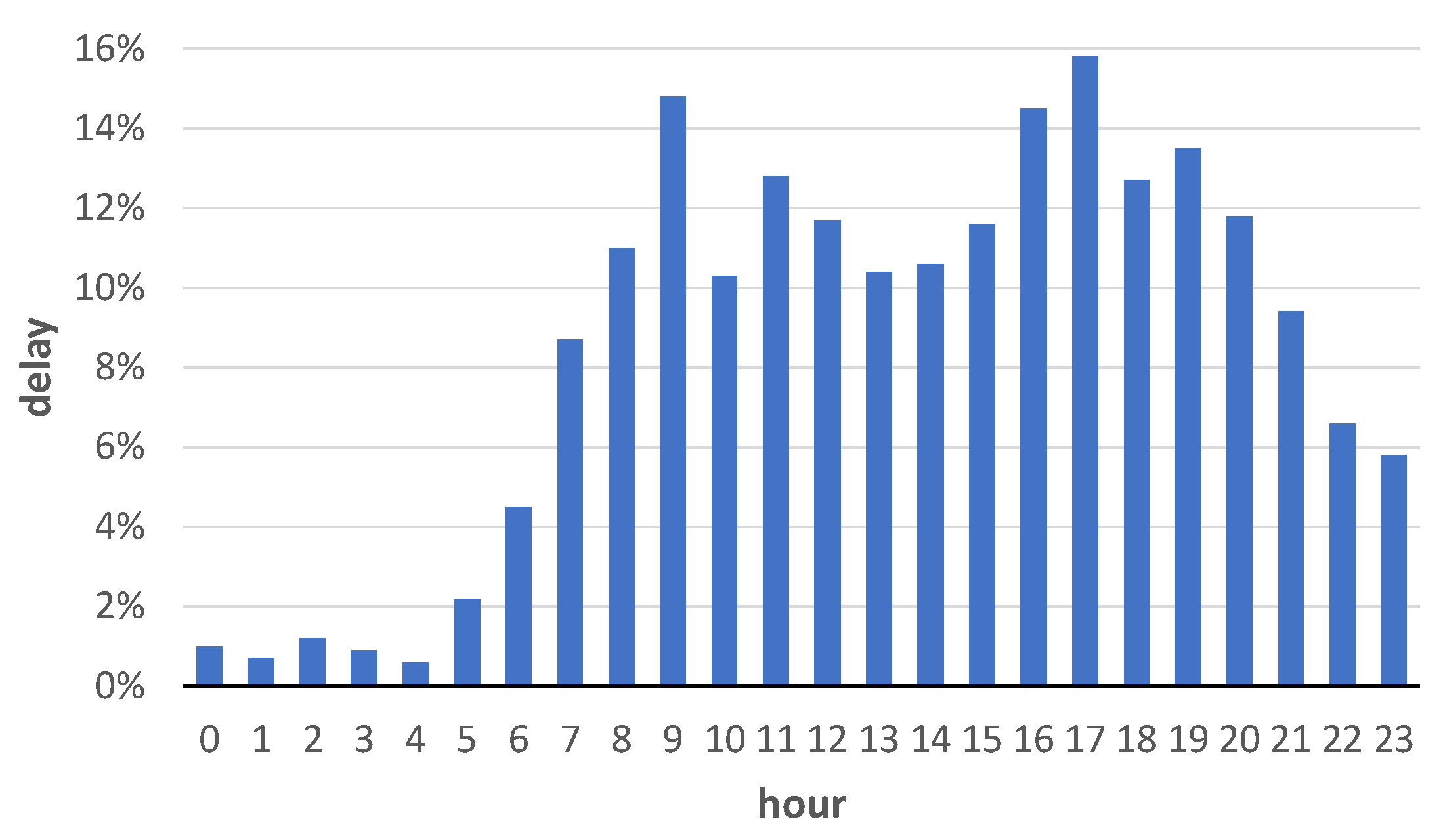
Figure 3.
Histogram of delays over the course of 24 h for weekends.
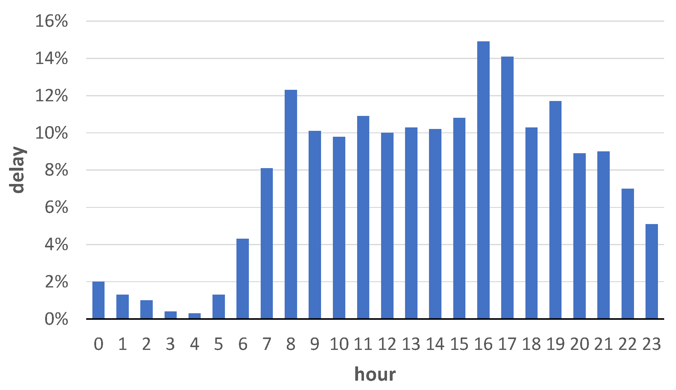
Figure 4.
Line 109: mean delays on Avenue 18 de Julio.

Figure 5.
Line 109: mean delays on Avenue 8 de Octubre.
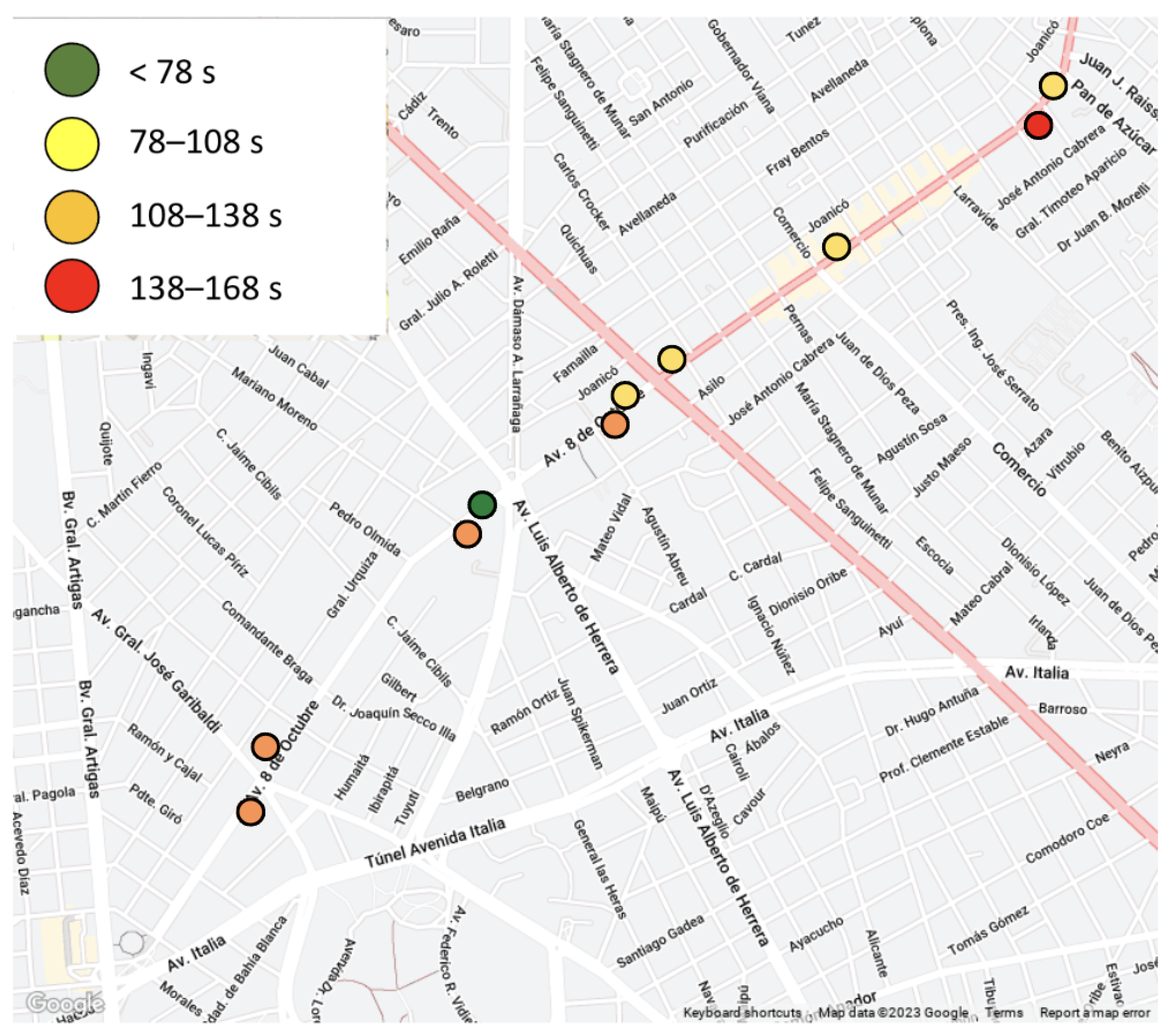
Figure 6.
Line 109: mean delays on Camino Carrasco.

Figure 7.
Line 181: mean delays on Avenue Luis Alberto de Herrera.

Figure 8.
Line 181: mean delays on Bulevar España and Bulevar Artigas: (a) Bulevar España (b) Bulevar Artigas.
Figure 8.
Line 181: mean delays on Bulevar España and Bulevar Artigas: (a) Bulevar España (b) Bulevar Artigas.
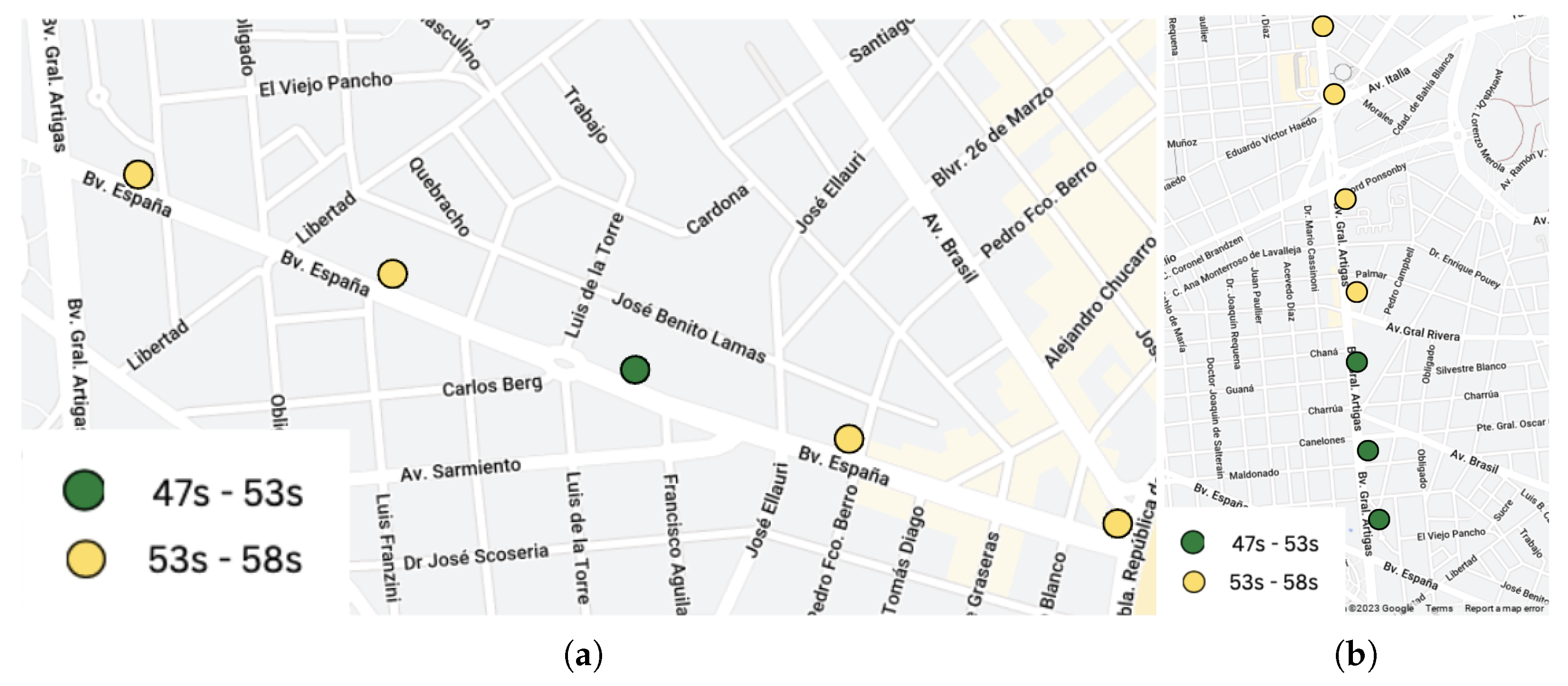
Figure 9.
Assignment of travel times to stops on the final stretch of line 2 from Hospital Saint Bois to Playa Malvín.
Figure 9.
Assignment of travel times to stops on the final stretch of line 2 from Hospital Saint Bois to Playa Malvín.
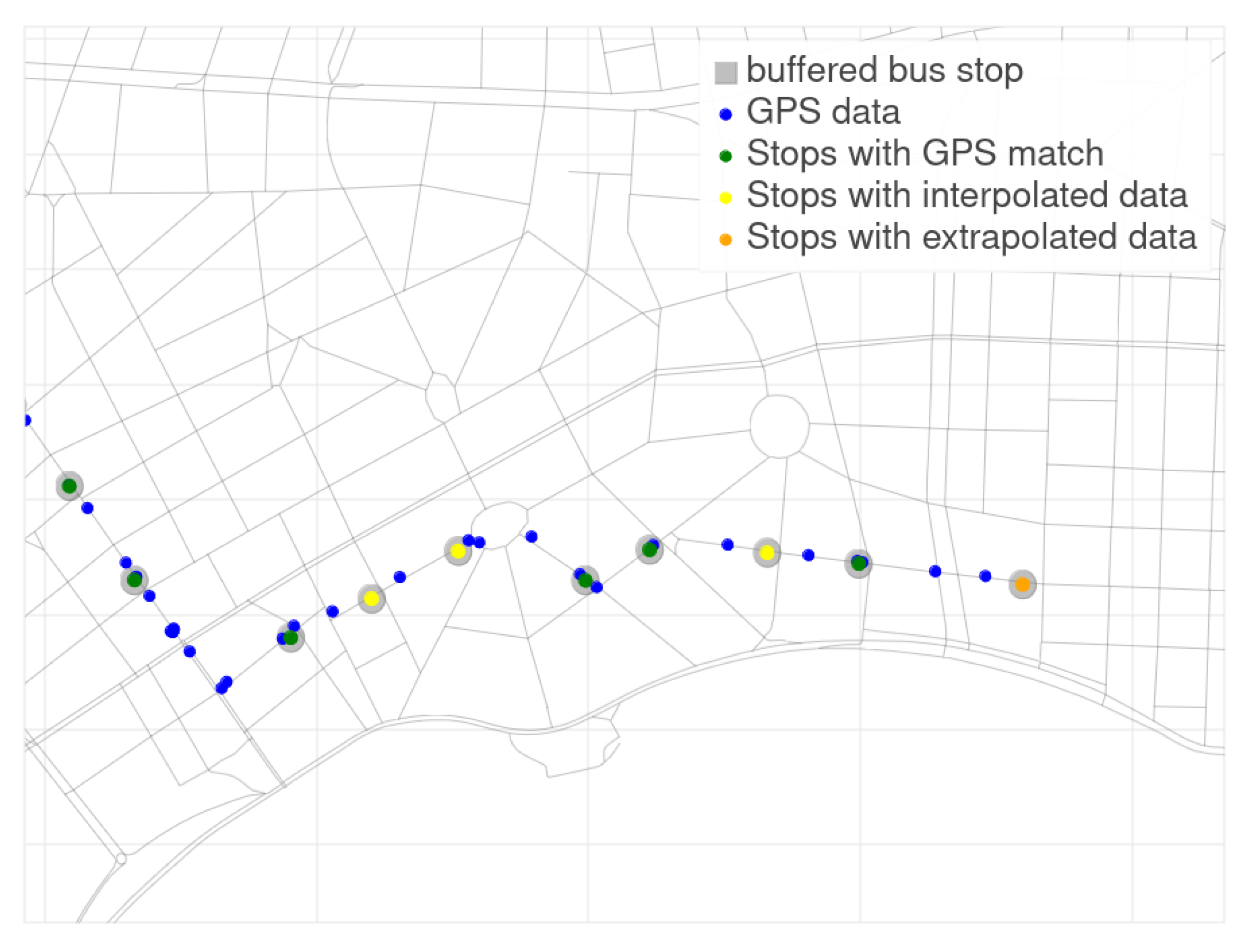
Figure 10.
Differences between the real and scheduled travel times (a) per trip and (b) median per line.
Figure 10.
Differences between the real and scheduled travel times (a) per trip and (b) median per line.
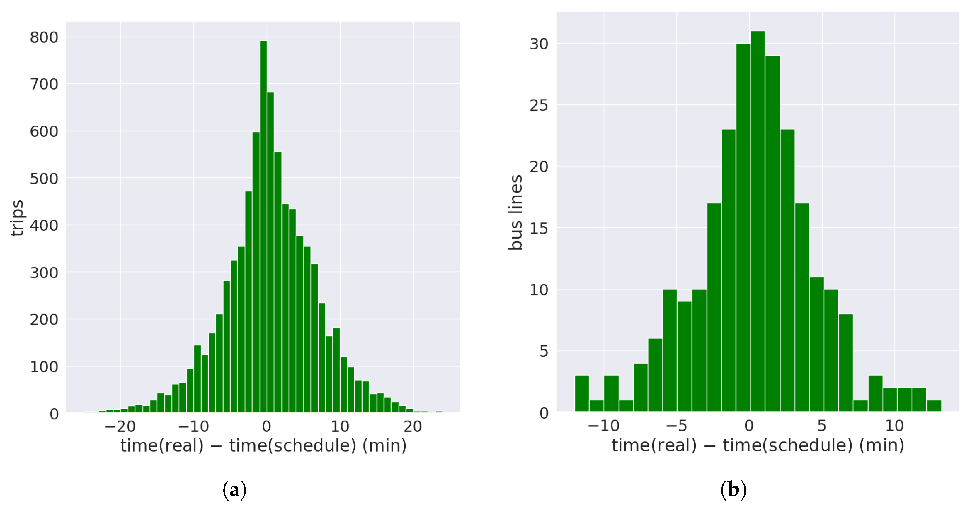
Figure 11.
Comparison of travel times (estimated vs. scheduled) for line 181.
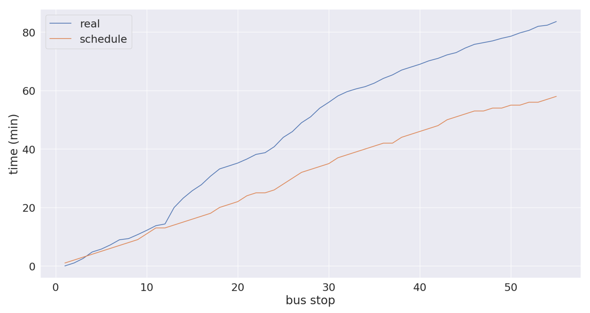
Figure 12.
Absolute difference of travel times (estimated vs. scheduled) for a trip on line 181.
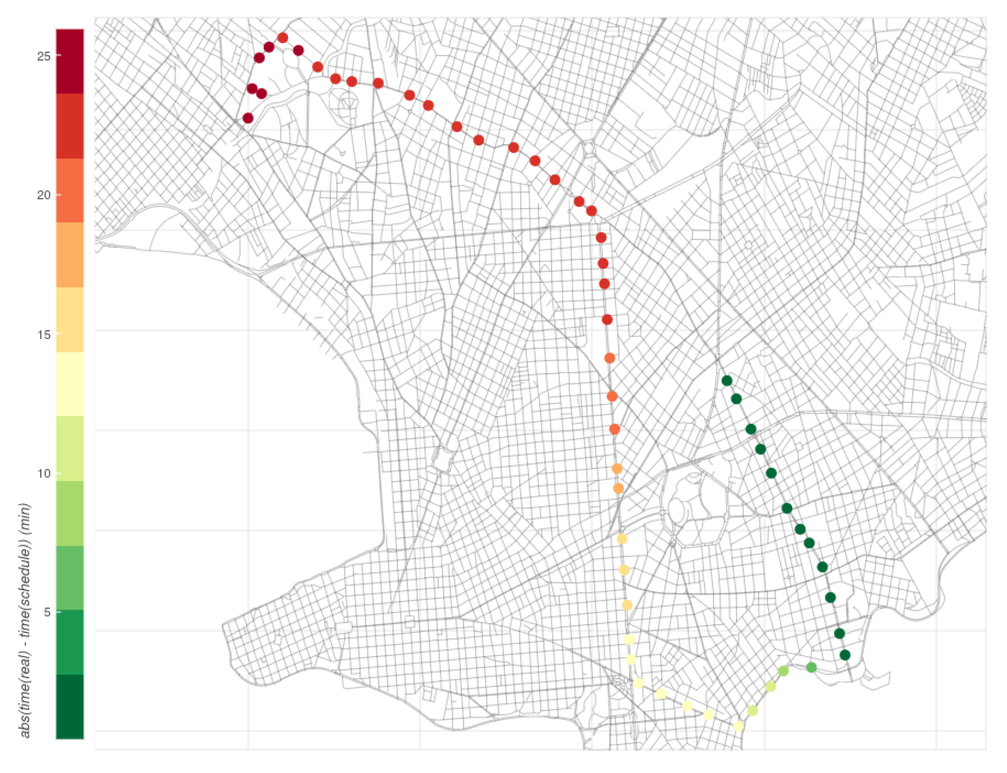
Figure 13.
Operational speed: (a) descriptive statistics and (b) histogram.
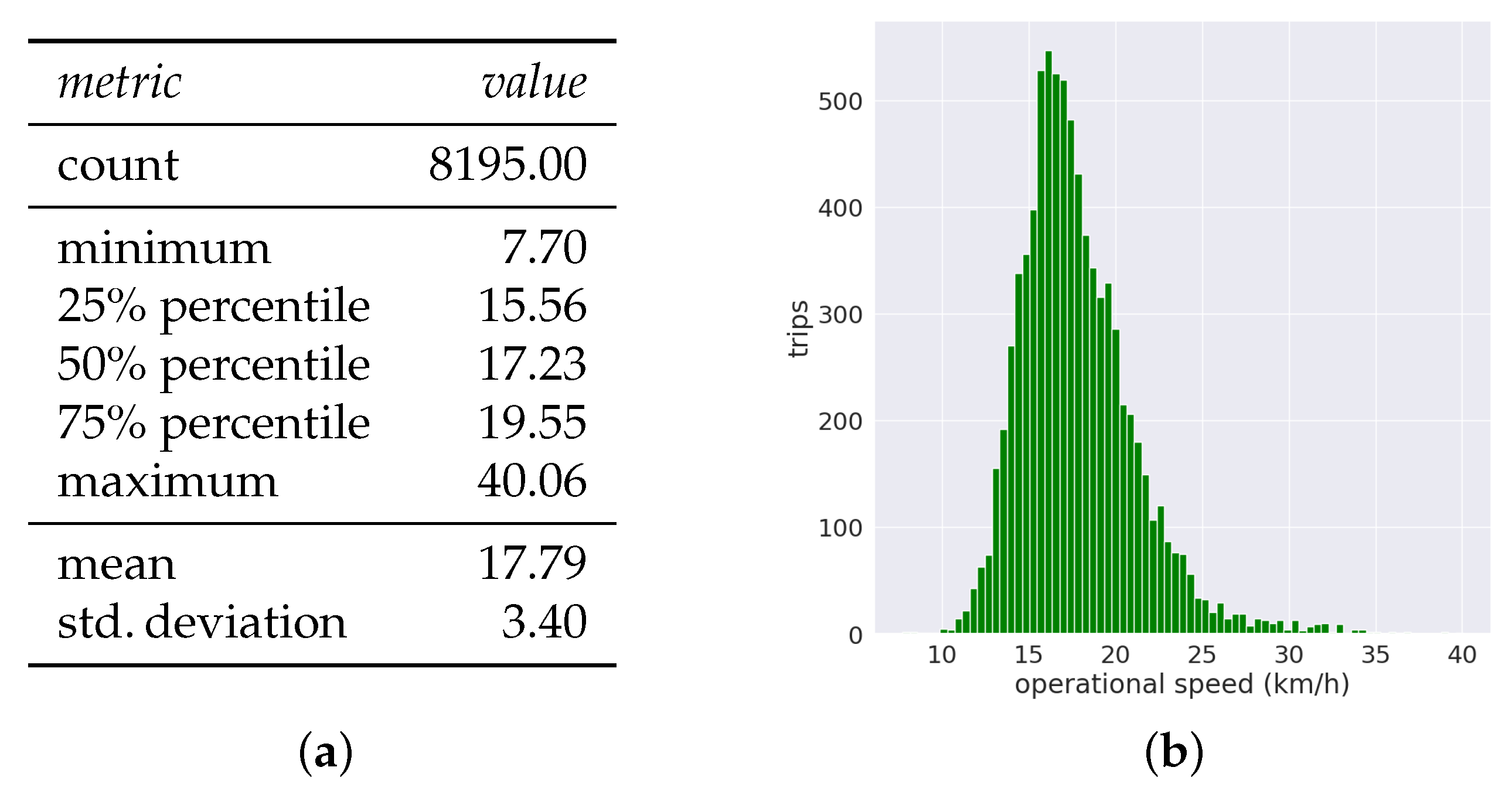
Figure 14.
OS dispersion: (a) descriptive statistics and (b) histogram.
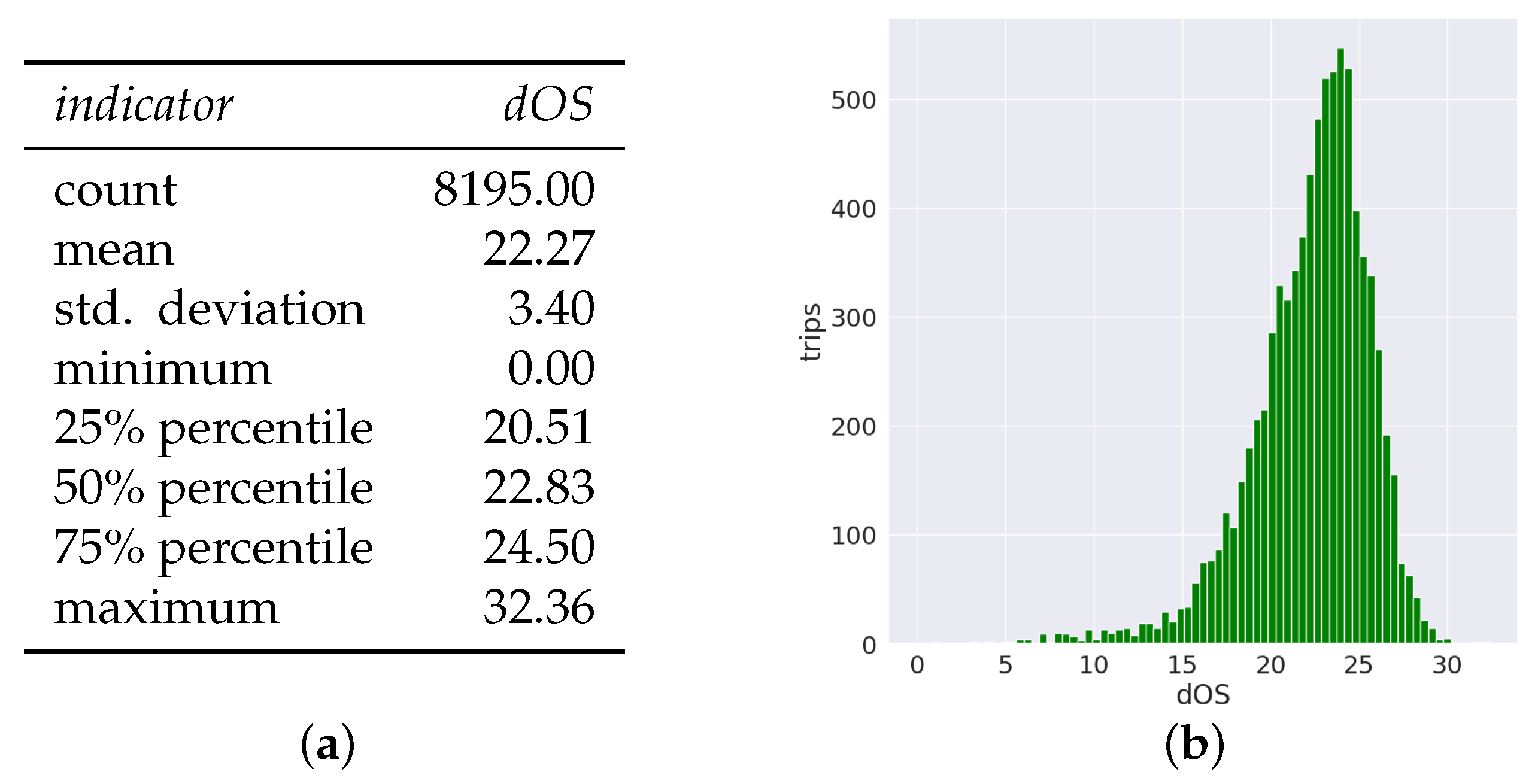
Figure 15.
OTAR results for bus lines: (a) indicators and (b) histogram.
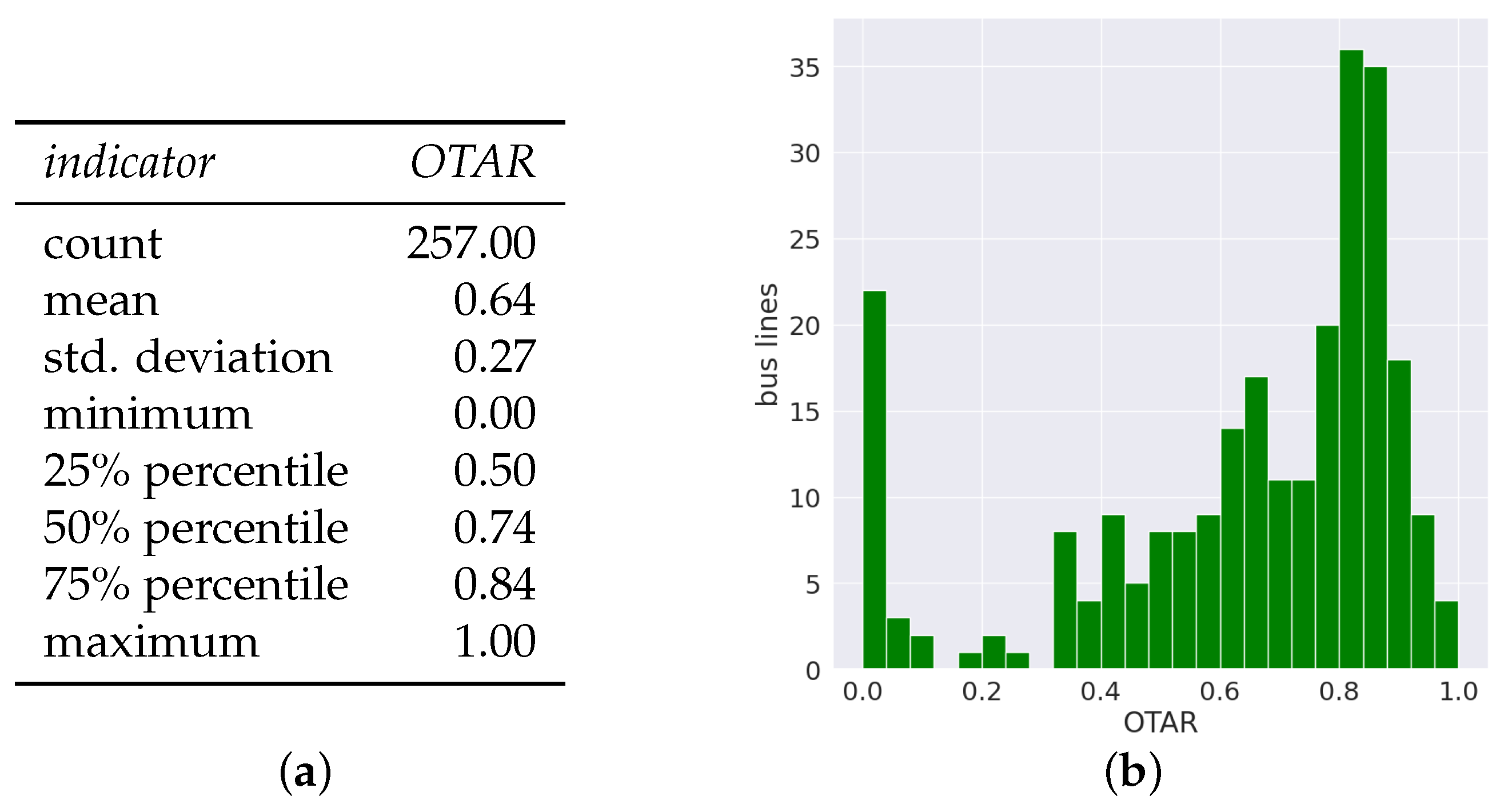
Figure 16.
ATToA of line 185 (origin Casabó, destination Pocitos).
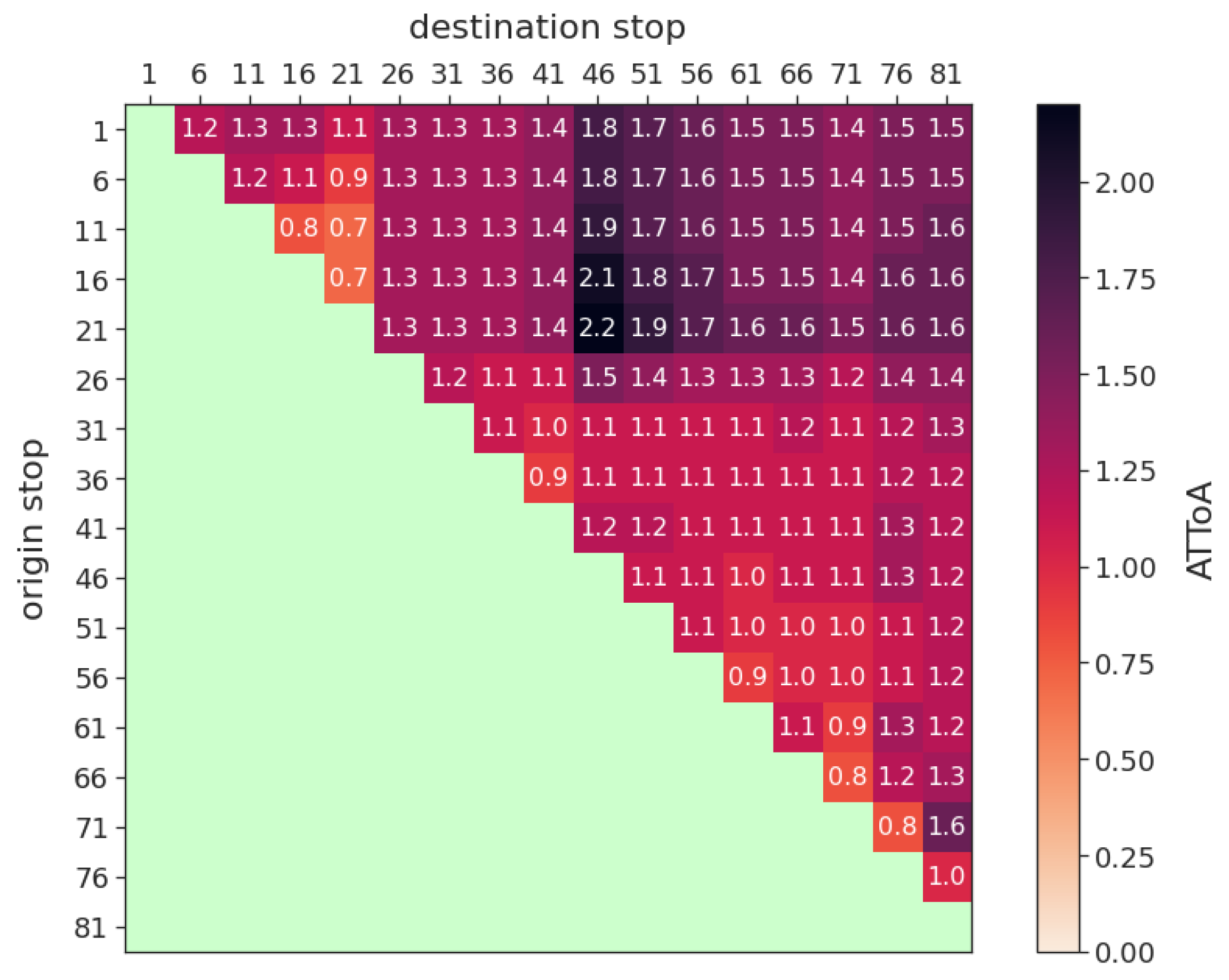

Table 1.
Comparison of delays for rush and non-peak hours.
| Avenue | Lines | Delay (s) | Mean Headway | Percentage | ||
|---|---|---|---|---|---|---|
| Rush Hours | Non-Peak | Rush Hours | Non-Peak | |||
| 18 de Julio | 38 | 116.91 | 115.77 | 842.86 | 13.9% | 13.7% |
| 8 de Octubre | 28 | 111.38 | 95.17 | 883.63 | 12.6% | 10.8% |
| Camino Carrasco | 14 | 95.60 | 77.69 | 913.59 | 10.5% | 8.5% |
| Luis Alberto de Herrera | 12 | 79.34 | 66.21 | 608.66 | 13.0% | 10.9% |
| Bulevar Artigas | 34 | 91.48 | 85.33 | 691.85 | 13.2% | 12.3% |
| Bulevar España | 12 | 92.77 | 75.17 | 882.77 | 10.5% | 8.5% |
Table 2.
Comparison of delays on weekdays and weekends.
| Avenue | Lines | Delay (s) | Mean Headway | Percentage | ||
|---|---|---|---|---|---|---|
| Weekend | Weekdays | Weekend | Weekdays | |||
| 18 de Julio | 38 | 115.51 | 115.11 | 1051.88 | 11.0% | 10.9% |
| 8 de Octubre | 28 | 101.32 | 110.50 | 1081.22 | 9.4% | 10.2% |
| Camino Carrasco | 14 | 84.96 | 111.97 | 1154.76 | 7.4% | 9.7% |
| Luis Alberto de Herrera | 12 | 71.91 | 74.91 | 707.75 | 10.2% | 10.6% |
| Bulevar Artigas | 34 | 87.59 | 75.44 | 847.61 | 10.3% | 8.9% |
| Bulevar España | 12 | 83.72 | 70.95 | 956.66 | 8.8% | 7.4% |
Table 3.
Mean delay values for lines 109 and 181.
| Line 109 | Line 181 | ||||
|---|---|---|---|---|---|
| Avenue | Delay (s) | Headway | Avenue | Delay (s) | Headway |
| 18 de Julio | 134.82 | 804.55 | Luis Alberto de Herrera | 53.24 | 384.83 |
| Camino Carrasco | 105.85 | 915.67 | Bulevar Artigas | 60.39 | 378.97 |
| 8 de Octubre | 93.09 | 936.53 | Bulevar España | 57.52 | 372.65 |
Table 4.
OTAR and percentage of trips with significant delays.
| Avenue | OTAR Buffer | Significant Delay | ||
|---|---|---|---|---|
| 2 min | 4 min | 5 min | ||
| 18 de Julio | 84.97% | 95.51% | 98.79% | 2.21% |
| Camino Carrasco | 87.08% | 95.65% | 98.50% | 1.50% |
| 8 de Octubre | 89.44% | 96.26% | 98.83% | 1.17% |
| Luis Alberto de Herrera | 88.74% | 95.53% | 98.81% | 1.19% |
| Bulevar Artigas | 84.78% | 94.80% | 97.76% | 2.24% |
| Bulevar España | 91.04% | 96.96% | 98.90% | 1.10% |
Table 5.
Buffer coefficients for OTAR: descriptive statistics.
| Indicator | Buffer |
|---|---|
| count | 257.00 |
| min | 0.00 |
| 25% | 0.08 |
| 50% | 0.11 |
| 75% | 0.14 |
| max | 0.38 |
| mean | 0.11 |
| std | 0.06 |
Disclaimer/Publisher’s Note: The statements, opinions and data contained in all publications are solely those of the individual author(s) and contributor(s) and not of MDPI and/or the editor(s). MDPI and/or the editor(s) disclaim responsibility for any injury to people or property resulting from any ideas, methods, instructions or products referred to in the content. |
© 2023 by the authors. Licensee MDPI, Basel, Switzerland. This article is an open access article distributed under the terms and conditions of the Creative Commons Attribution (CC BY) license (https://creativecommons.org/licenses/by/4.0/).
Share and Cite
MDPI and ACS Style
Nesmachnow, S.; Massobrio, R.; Guridi, S.; Olmedo, S.; Tchernykh, A. Big Data Analysis for Travel Time Characterization in Public Transportation Systems. Sustainability 2023, 15, 14561. https://doi.org/10.3390/su151914561
AMA Style
Nesmachnow S, Massobrio R, Guridi S, Olmedo S, Tchernykh A. Big Data Analysis for Travel Time Characterization in Public Transportation Systems. Sustainability. 2023; 15(19):14561. https://doi.org/10.3390/su151914561
Chicago/Turabian StyleNesmachnow, Sergio, Renzo Massobrio, Santiago Guridi, Santiago Olmedo, and Andrei Tchernykh. 2023. "Big Data Analysis for Travel Time Characterization in Public Transportation Systems" Sustainability 15, no. 19: 14561. https://doi.org/10.3390/su151914561
Note that from the first issue of 2016, this journal uses article numbers instead of page numbers. See further details here.