Article

In Pursuit of Local Solutions for Climate Resilience: Sensing Microspatial Inequities in Heat and Air Pollution within Urban Neighborhoods in Boston, MA

by
Daniel T. O’Brien
1,2,3,* and
Amy V. Mueller
4,5
1
School of Public Policy and Urban Affairs, Northeastern University, Boston, MA 02115, USA
2
School of Criminology and Criminal Justice, Northeastern University, Boston, MA 02115, USA
3
Boston Area Research Initiative, Northeastern and Harvard Universities, Boston, MA 02115, USA
4
Department of Civil and Environmental Engineering, Northeastern University, Boston, MA 02115, USA
5
Department of Marine and Environmental Sciences, Northeastern University, Boston, MA 02115, USA
*
Author to whom correspondence should be addressed.
Sustainability 2023, 15(4), 2984; https://doi.org/10.3390/su15042984
Submission received: 16 November 2022 / Revised: 30 January 2023 / Accepted: 31 January 2023 / Published: 7 February 2023
(This article belongs to the Special Issue Human Behavior, Urban Health and Sustainability)

Abstract

:
Environmental hazards vary locally and even street to street resulting in microspatial inequities, necessitating climate resilience solutions that respond to specific hyperlocal conditions. This study uses remote sensing data to estimate two environmental hazards that are particularly relevant to community health: land surface temperature (LST; from LandSat) and air pollution (AP; from motor vehicle volume via cell phone records). These data are analyzed in conjunction with land use records in Boston, MA to test (1) the extent to which each hazard concentrates on specific streets within neighborhoods, (2) the infrastructural elements that drive variation in the hazards, and (3) how strongly hazards overlap in space. Though these data rely on proxies, they provide preliminary evidence. Substantial variations in LST and AP existed between streets in the same neighborhood (40% and 70–80% of variance, respectively). The former were driven by canopy, impervious surfaces, and albedo. The latter were associated with main streets and zoning with tall buildings. The correlation between LST and AP was moderate across census tracts (r = 0.4) but modest across streets within census tracts (r = 0.16). The combination of results confirms not only the presence of microspatial inequities for both hazards but also their limited coincidence, indicating that some streets suffer from both hazards, some from neither, and others from only one. There is a need for more precise, temporally-dynamic data tracking environmental hazards (e.g., from environmental sensor networks) and strategies for translating them into community-based solutions.

1. Introduction

Climate change is a global phenomenon, but its associated environmental hazards and their health impacts are experienced locally. Within a single coastal city, for instance, some communities are closer to the shore, exposing them more directly to flooding (e.g., [1,2]); some have infrastructure that contributes more to urban heat island development, making them more vulnerable to extreme heat events and consequent medical emergencies (e.g., [3,4,5,6]); some experience heavier usage of transportation, potentially creating concentrations of air pollution and thus respiratory disease [7,8,9]; and so on. Thus, equitable pathways to sustainability in urban environments will require locally tailored solutions that incorporate the unique context, conditions, and priorities of each community. Arriving at such solutions will require granular data that allow stakeholders and decision makers to identify and track microspatial inequities in environmental hazards—that is, disparities in exposure to conditions like extreme heat, air pollution, flooding, and others that vary at hyperlocal scales, such as street-to-street within communities. Emergent technologies, especially networks of environmental sensors, provide the opportunity to characterize such disparities at high spatial resolution, revealing the landscape of hazards in a community and providing a literal map for action. To date, however, such systems are cost-prohibitive, and our limited understanding of microspatial inequities means we are ill-equipped to unlock their transformative potential. The goal of this paper is to use existing remote sensing data, which is less precise and more dependent on proxies than data from local sensor networks, in concert with catalogued information about the cityscape itself, to present initial evidence for the distribution of microspatial inequities in heat and air pollution across the communities of Boston, MA, including the extent to which these two hazards overlap. This will provide a basis for further investigation on the subject and consequences, including health outcomes, as well as potential guidance for how sensor networks might be leveraged to improve current limitations to tracking hazards and informing community-based solutions.
Sensor networks have been lauded by “smart cities” enthusiasts as a technology of the future, a veritable “fitness tracker for the city” [10]. Environmental sensor networks consist of nodes (i.e., boxes housing sensor hardware and needed auxiliaries such as power or communications) placed throughout a community or city to measure environmental conditions, often in real time. Each node may incorporate multiple types of sensors, including temperature, wind speed and direction, precipitation, noise, various forms of air pollution, or solar insolation, among others. Sensor nodes sometimes include a camera that permits the tabulation of pedestrian, bicycle, and vehicle traffic. As such, sensor nodes have the capability to estimate the landscape of multiple hazards and at sufficient spatial density to capture not only disparities between communities but also the microspatial inequities that occur within communities, even from street to street.
Environmental sensor networks of some type have been rolled out in a few forward-looking cities, including Chicago, Berkeley, CA, and London [11,12,13], but they have otherwise gained limited traction. This stands in contrast to the popularity of other uses of sensors, most notably for tracking or responsively controlling the patterns of transit and transportation networks. However, the high cost of individual nodes and failure to date to identify a clear value proposition for local communities have discouraged many cities from investing in them. This creates a notable paradox. Owing in part to the lack of environmental sensor networks, there is a lack of evidence of microspatial inequities to justify the need to build such networks to track them. There is also a lack of guidelines to leverage typical patterns of hazard distribution to create cost-efficient network designs that optimize the placement of fewer sensors while still modelling disparities across space in a transparent and reliable way. All of these technical challenges must be overcome to enable the possibility of data-driven policymaking, practice, and community conversations.
If we are to develop local climate resilience solutions that counteract microspatial inequities impacting health and wellbeing, we must first come to understand their extent and severity in urban environments. Though there have been very few studies on the subject, microspatial inequities are likely to exist for most environmental hazards given what we know about their underlying drivers, which are often rooted in geophysical processes (i.e., air and water movement) that operate hyperlocally and in conjunction with the structure of the urban canopy (i.e., buildings and vegetation), which often varies from lot to lot. This is substantially different from social processes that are theorized to operate broadly at the neighborhood scale, creating consistent dynamics across the spaces of a community [14,15,16,17], though see [18] for a critique. Unfortunately, data availability has often limited in situ studies of environmental hazards to the examination of neighborhoods and even regions [19]. Though such work can be broadly informative, its interpretation may suffer from the ecological fallacy if it assumes that neighborhood-level variation is in fact the result of neighborhood-level processes. It may instead be that urban planning decisions partially segregate land use and infrastructure by neighborhood [20,21,22], giving the impression that neighborhood-level processes drive environmental hazards when in fact hyperlocal processes are likely an important factor.
We might illustrate the role of hyperlocal processes with extreme heat. The urban heat island effect is driven by the density of pavement, which absorbs heat; lack of trees, which otherwise would protect from sunlight and cool the air via evapotranspiration; and few reflective surfaces, which limit additional absorption of light energy (i.e., reflection of light energy; [23,24,25,26]). These features vary substantially between neighborhoods, creating temperature differences within a single city [27,28,29,30]. Of course, there are some geophysical processes that have the potential to diffuse throughout the neighborhood. For example, because the vegetative canopy cools the air via evapotranspiration it might lead to lower temperatures in surrounding areas as well, albeit with a diminishing effect with distance. Applying the same reasoning to air pollution, vehicular traffic, especially diesel freight delivery, generates the vast majority of air pollution on city streets, however the experience of these risk factors depends on whether the pollution is “flushed” into the upper atmosphere [31] or remains trapped in the boundary layer where humans live and move. The latter is most likely along narrow streets with tall buildings owing to the “urban canyon effect”, a regime that can be precisely defined using fluid mechanics framing [32,33]. Additionally, elements of localized heating [32] and tree canopy [34] can also be important drivers of the precise level of flushing experienced in any street segment.
A second consideration for understanding microspatial inequities is the extent to which environmental hazards overlap. Neighborhood researchers from various fields, including sociology, criminology, and public health, have long observed that various undesirable conditions and outcomes tend to cluster together, from poverty to crime to mental and physical health to education to economic opportunity [14,15,16,17,35]. Advocates for environmental justice have similarly noted that communities with more resources leverage money and political power to distance themselves from all types of environmental hazards—which in turn results in marginalized groups being consistently exposed to more environmental hazards [19,20,36]. This dynamic is often visible in the placement of airports, highways, and power plants or the use of banking practices to channel investment in particular ways [6,37,38,39,40]. It is not clear, however, that each such decision will impact all environmental hazards for all low-income or majority-minority neighborhoods. For example, an airport will create more air pollution and noise for the surrounding community but may not have similar implications for heat or flooding. This raises the question of whether environmental hazards correlate strongly across neighborhoods, an assertion that has surprisingly almost never been tested (see [41] for a rare example). Meanwhile, if we return to the idea that environmental hazards are governed at hyperlocal scales by geophysical processes, the extent to which they overlap within neighborhoods will depend on the extent to which their underlying drivers coincide. In the case of heat and air pollution, there appears to be a shared connection to major streets, which have both pavement and high traffic, but other drivers (e.g., vegetative cover) may disrupt this correlation. As such, we might expect to see a mosaic of microspatial inequities across the streets of a neighborhood, some with high heat, others with high air pollution, some with both, and some with neither.
Here we present a case study evaluating the extent to which (1) heat and air pollution give rise to microspatial inequities within neighborhoods and (2) these hazards have distinct or overlapping distributions that result in various combinations of exposure across a neighborhood’s streets. This moves beyond existing work on these environmental hazards in cities, which has largely emphasized how neighborhood-level variations for both the urban heat island effect [6,27,28,29,30,42,43] and air pollution [21,44] affect health outcomes. A sole exception found that extreme heat indeed varied street-to-street within neighborhoods, driven by differences in tree canopy, impervious surfaces, and albedo. Further, they demonstrated that these variations—not neighborhood-level variations—best explained geographic disparities in medical emergencies during heat advisories [45]. Meanwhile, Gately et al. [46] estimated vehicle-generated emissions street-by-street, presenting a series of maps that offer preliminary evidence for the potential generation of microspatial inequities. That said, they stopped short of modeling the importance of streets in capturing variance and only estimated emissions, which, as noted, drive elevated concentrations only when they are not flushed by airflow. Meanwhile, as noted, very few studies have examined the extent to which environmental hazards overlap (i.e., correlate) across neighborhoods, and none that we know of have done so across streets within neighborhoods.
The current case study specifically examines Boston, MA, owing to (1) documented evidence of high variability in hazards between the city’s neighborhoods, (2) variability in urban infrastructure and form throughout the city, increasing the likelihood of microspatial variability, and (3) a wealth of available data, including GIS inventories of roads, buildings, and land cover, and resources for estimating both temperature and air pollution. It is important to note, however, that these latter resources are imperfect substitutes for the direct measures generated by in-situ studies or environmental sensor networks, which are not available for Boston. Instead, they are calculated using proxies in conjunction with a physics-based understanding of the role of urban infrastructure to generate a best-available estimate of parameter distribution. The results are a first-pass approximation that likely captures spatial variation while being imprecise in terms of their absolute values. Further, they fail to capture fluctuations across seasons and weather conditions. While we do not believe these limitations undermine the analysis and its overarching insights, they do force us to present only relative comparisons and not to delve into the implications of absolute measures (e.g., identifying thresholds for health impact concerns). That said, provided we find support for our hypotheses, the weaknesses of the data highlight the potential advantages that high resolution environmental data, whether from sensor networks or other technologies, could provide for communities over such proxy-based data sets. We return to this in the Section 4.
The study proceeds in two parts. First, we map estimated ambient levels of air pollution and extreme heat for all streets in the city, quantifying the extent to which variation is distributed across streets or neighborhoods. Second, we leverage detailed information on infrastructure to identify the drivers of both hazards at the street and neighborhood levels. Third, we examine the correlations between estimated air pollution and heat across neighborhoods and across streets within neighborhoods, conducting the first test of multihazard exposure at the microspatial scale.

2. Materials and Methods

2.1. Data Sources and Processing

The study leverages three data sources. First, the Urban Heat Island Database [23,47] documents land surface temperature and associated environmental characteristics derived from remote sensing data for 30 m × 30 m grid cells across greater Boston. Second, Gately et al. [46,48] made high resolution estimates of air pollutant emissions from vehicles available for greater Boston. Third, we coordinated and supplemented these two data sets of hazards using the Boston Area Research Initiative’s (BARI) Geographical Infrastructure for Boston (GI) [49], which links all land parcels (i.e., addresses) identified in the City of Boston’s Tax Assessments to U.S. Census TIGER line street segments (i.e., the undivided length of street between two intersections or an intersection and a dead end) and nests them within census tracts. In addition to enabling the coordination of measures from the two other data sets for all street segments (see below for more), it provided other descriptors of the land use and structure of the City’s streets and neighborhoods. There are 24,757 street segments in Boston’s 178 census tracts. Of these, 24,579 had measures for all components of the Urban Heat Island database’s grid, comprising the sample for all analyses of the distribution of heat; 12,954 had information sufficient to estimate air pollution (in 177 census tracts; see below for inclusion criteria), comprising the sample for all analyses of the distribution of air pollution; all but 18 street segments with measures for air pollution also had a measure for heat, comprising a sample of 12,936 street segments in 178 census tracts for analysis of the overlap between the two hazards. See Table 1 for descriptive characteristics for all variables.

2.1.1. Land Surface Temperature and Associated Factors

The Urban Heat Island Database [47] contains four measures for each 30 m × 30 m grid cell in Boston, drawn from multiple sources. Land surface temperature was estimated by combining Landsat 5 TM 120 m and Landsat 7 ETM+ 60 m brightness temperature observations in summer intervals (1 June–31 August) from 2002 to 2008. Brightness temperature data were screened for clouds [50] and atmospherically corrected for scattering and haze effects [51]. Brightness temperature was then converted to land surface temperature and downscaled to 30 m by estimating emissivity values from 30 m surface reflectance data [52]. Landsat data are collected at 10:20 a.m. local time. Note that temperatures are somewhat higher than one might expect as land surface temperature is typically 5–11 °F higher than the air temperature experienced by people (mean = 98.55 °F for streets).
In addition to land surface temperature, the database included three closely related environmental characteristics. Albedo, or surface reflectivity, was calculated on a scale from 0–1 (mean = 0.13 for streets) from combined Landsat (30 m) and MODIS (500 m) observations in summer intervals (1 June–31 August) from 2003 to 2008 at approximately 10:20 a.m. local time to produce 30 m raster cells [53]. Canopy fraction corresponding approximately to the year 2010 was obtained from the 30 m National Land Cover Database (from 0–1; mean = 0.10) [54]. Impervious surface cover fraction was aggregated to 30 m pixels from a 1 m grid generated by orthophotography data provided by MassGIS for 2015 by mean value per pixel (from 0–1; mean = 0.77).

2.1.2. Air Pollution Concentration

Gately et al. [48] approximated air pollution emissions across the streets of eastern Massachusetts by estimating traffic volume and speed drawn from cellphone-generated mobility data and combining with established relationships between vehicle speed, type, and emission levels [46]. These were calculated for all street segments and then converted to rasters with grid cells of approximately 75 m. The many indicators of air pollution are highly inter-correlated, so we use carbon monoxide (CO) as the proxy for overall vehicle emissions of airborne pollutants in the generation of the heterogeneity map for estimated air pollution levels.
Exposure to air pollution depends critically not only on vehicle emissions but also how local air flow dynamics disperse or trap them. Based on current understandings of the fluid dynamics of urban canyons [32,33] we approximated the street segment flushing regime (low, moderate, high) using the average height of buildings of each street (approximated as 4 m per floor) and the street width (based on estimates from Mass Highway department; see below for more on these measures) to estimate the urban canyon aspect ratio (street width divided by building height, or W/H). Streets that are wider or have shorter buildings (or empty lots), i.e., the ratio of street width to building height is higher, have higher flushing rates (i.e., more air flow and therefore lower pollution concentrations) while streets that are narrower or have taller buildings have lower flushing rates and therefore higher potential to concentrate locally-emitted pollution. Cutoff between regimes is dictated by fluid dynamics system properties based on width-to-height ratio (W/H). Specifically, W/H < 1.54 is low flushing (sheer at top of canyon drives flushing to the atmospheric boundary layer), 1.54 < W/H < 6.67 is moderate flushing (turbulent eddies in the canyons dominate flushing), and W/H > 6.67 is high flushing (atmospheric boundary layer essentially reaches to ground level). Given the limitations of the available data, rather than attempt to estimate actual ambient air pollution concentrations, we instead classify each street segment based on likely risk level by combining emissions and flushing estimates. Low risk is indicated by a below average emissions rate or a high flushing rate. Medium risk falls between the 50th and 75th percentile in emissions and has moderate flushing or is over the 75th percentile in emissions but with a high flushing rate. High risk falls between the 50th and 75th percentile in emissions and has a low flushing rate or is over the 75th percentile in emissions and has a moderate or low flushing rate. See Land Use for calculation of W/H.

2.1.3. Land Use

The Geographical Infrastructure (GI) provided information on urban form that may be correlated with both the experience of land surface temperature (i.e., owing to the thermal properties of buildings and spaces) [55] and air pollution (i.e., by influencing traffic patterns or airflow). These include its classification as a Main street (i.e., a thoroughfare above a certain width that is short of a highway; provided by MassGIS), and primary land usage (a seven-group typology based on a cluster analysis of the representation of each land use; see Table 1). We calculated width-to-height ratio of a street and its buildings (W/H) by estimating building heights from the number of floors in each building on a street (from Boston’s tax assessments; approximating 4 m per floor) and the street width from the number of lanes (based on classifications from MassGIS (e.g., limited access highway vs. major arterial vs. minor road) and information from MassHighway on the structure of these types, with lanes estimated as 6.15 m, shoulders as 4.1 m, and sidewalks as 2–3 m depending on road type). This calculation was limited to street segments with at least one parcel with a stated number of floors, because otherwise we could not account for the presence of building whose address did not place it officially on that street segment, leaving 12,954 street segments. We excluded 11,059 street segments with no parcels and 878 street segments with no parcels with a recorded number of floors (638 of which were dominated by building zoned as exempt, which often contain less information in tax assessments because they are not formally taxed). Last the GI includes population density for each census tract (from the US Census Bureau’s American Community Survey) and classifies each as being primarily residential, downtown, institutional (e.g., industrial, university), or centered on a large park.

2.1.4. Data Coordination

The Urban Heat Island database and the air pollution data were both provided as rasters. To extract measures of LST, albedo, canopy, impervious surfaces, and air pollution for each street segment, we calculated the proportion of each street segment in Boston contained in each raster grid cell. This was then used to create a weighted average of these five measures of the environment on each street segment. We followed the same process for census tracts. For the urban heat island database, rather than average values for all streets in each census tract, we weighted all grid cells falling within the tract, because we would otherwise have ignored areas not on streets. This provides a more comprehensive measure of the census tract environment. This was not relevant for the air pollution data, which specifically measured emissions on streets and did not have data for other spaces. These street and tract measures were then merged with the land use descriptors at each level provided by the GI. Street segments were attributed to the census tract in which the majority of their land parcels fell, a logic necessary to classify street segments forming the border between census tracts.

2.2. Analysis

The main analysis occurs in two parts. First, we decomposed variance between streets and tracts using ANOVAs wherein tracts act as the grouping (i.e., independent) variable. These estimated the percentage of variance at each level. We then ran multilevel models that nested street segments within tracts (by the logic described in Data Coordination; see Data Sources and Processing for sample sizes). The models simultaneously test the effects of factors at each geographic scale while holding features of the other level constant, taking the form:
Y j k = β 0 k + β 1 k × x ( 1 ) j k + + β n k × x ( n ) j k + r j k   Street   Equation  
β 0 k = γ 00 + γ 01 × x ( 01 ) k + + γ 0 n × x ( 0 n ) l + μ 0 k   Tract   Equation  
where β and γ are parameter estimates for predictors at the street and tract levels, respectively, and r and μ are error terms at the street and tract levels, respectively. Tract-level parameters quantify the effect of a given factor on all streets in a census tract. Y j k is the value of the dependent variable for the jth street in the kth census tract. Yjk is either land surface temperature or air pollution, depending on the model. The first is a normally distributed variable, permitting the use of an identity link. The latter is a categorical variable, in which case we predict a street being at either moderate- or high-risk for air pollution exposure as a dichotomous variable, necessitating a binomial link. These are both run in the lme4 package in R [56].

3. Results

3.1. Descriptive Statistics

The average street had an LST of 98.6 °F (as noted in the Methods, land surface temperature is typically higher than the experienced air temperature by 5–11 °F). This varied substantially, however, from 72.4 °F to 116.4 °F. Half of streets fell between 95.4 °F and 102.6 °F. This distribution is only moderately narrowed when considering census tracts, whose average temperatures range from 87.4 °F to 106.4 °F. Consistent with this, the average neighborhood had a difference of 15 °F between its hottest and coolest streets—nearly double the difference between the 25th and 75th quartile of streets in the city. In 37 census tracts (21%), this range was over 20 °F.
For air pollution exposure, 61% of streets were classified as low risk, 27% as medium risk, and 12% as high risk. The proportions of street segments at each risk level varied considerably geographically, however, with neighborhoods ranging from 96% to near 0% of streets being low-risk (limited to 155 tracts with 20 or more street segments to prevent outliers.). Approximately half of neighborhoods had between 44% and 79% low-risk streets. In sum, the initial statistics for LST and air pollution point to considerable variation both within and between tracts for both hazards, as represented geographically in Figure 1. How this might look among the streets of a single census tract is also presented in Figure 2a,b.

3.2. Distribution of Hazards across Streets

As noted above, the analysis sought to better understand the distribution of LST and air pollution in two stages. First, ANOVA models partitioned the variance in each hazard between the street and tract levels. Second, we ran multilevel models that incorporated independent predictors at first the street and then the tract level to assess the factors that most drive the distribution of these hazards. We present the results for heat first and then for air pollution. See Table 2 for all predictors and parameter estimates.

3.2.1. Land Surface Temperature

An initial ANOVA found that 39% of the variation in temperature occurs between streets in the same neighborhood. To explain this variance, we first incorporated the characteristics of streets into multilevel models, focusing on the three infrastructural elements most often cited as driving the urban heat island effect: tree canopy, impervious surfaces, and albedo. It is worth noting that each of these components, particularly tree canopy, may indirectly factor into the way land surface temperature is estimated because of their effect on emissivity, which is the primary proxy for calculating land surface temperature from LandSat data.
All three infrastructural elements were major predictors of street temperature (all p-values < 0.001). An increase in canopy cover by 10% predicted a drop in temperature by 1.5 °F, an increase in impervious surfaces by 10% predicted a temperature that is 0.7 °F higher, and an increase in albedo of 1% (approximately practically comparable to a change of 10% in canopy), equated to an expected drop in temperature of 0.2 °F. Crucially, these predictors not only explained 40% of the variation between streets within neighborhoods but also accounted for 74% of variation between neighborhoods, meaning that between-neighborhood variance appears to have been largely a function of streets with similar features being clustered together. This result is partially illustrated by the visible relationship between canopy and street temperature in an example neighborhood in Figure 2.
A final model tested the additional impact of tract-level measures of canopy, pavement, and albedo, which could occur if such features influence temperatures in nearby spaces. The level of canopy cover and impervious surfaces were predictive at this higher level as well, albeit at a more modest scale than at the street level. A 10% increase in canopy cover predicted an increase of 0.7 °F (p < 0.001), and a 10% increase in impervious surfaces predicted an increase of 0.4 °F (p < 0.001). Albedo at the tract level had no independent effect. These factors accounted for 10% of additional variation between neighborhoods.

3.2.2. Air Pollution

Census tracts accounted for 20% of the variation in the locations of streets we estimated to be at medium or high risk for air pollution and 28% of the variation in streets we estimated as high risk. As such, 70–80% of the variation in air pollution risk lies between streets in the same neighborhood, which is approximately double that seen for LST. To explain this variation, our models focused on infrastructural elements that might account for traffic and airflow. At the street level, we tested whether predominant land use (e.g., residential) and being a main street or dead end predicted air pollution. Land use was an especially strong predictor. Streets dominated by single-family housing had the least risk of having moderate or high pollution. At the other end of the scale, streets dominated by commercial and mixed-use commercial buildings were 3.74 and 5.75 times as likely to be at risk for air pollution, respectively (p-values < 0.001). In between were streets with higher density housing, like condos, apartment buildings, and three-family houses, which tended to be about twice as likely to be at risk than streets predominated by single-family housing. Meanwhile, main streets were nearly 40 times as likely to be at risk for air pollution, independent of their land use, likely owing to greater traffic flow and taller buildings (p < 0.001). This effect is illustrated by maps from an example neighborhood in Figure 2.
We then introduced population density and a four-category classification of neighborhood use as additional predictors. The only significant factor was that “downtown” neighborhoods had substantially higher risk than other types of neighborhoods, especially residential neighborhoods (B = 1.37, O.R. = 3.94, p < 0.001), likely owing to a density of tall buildings.

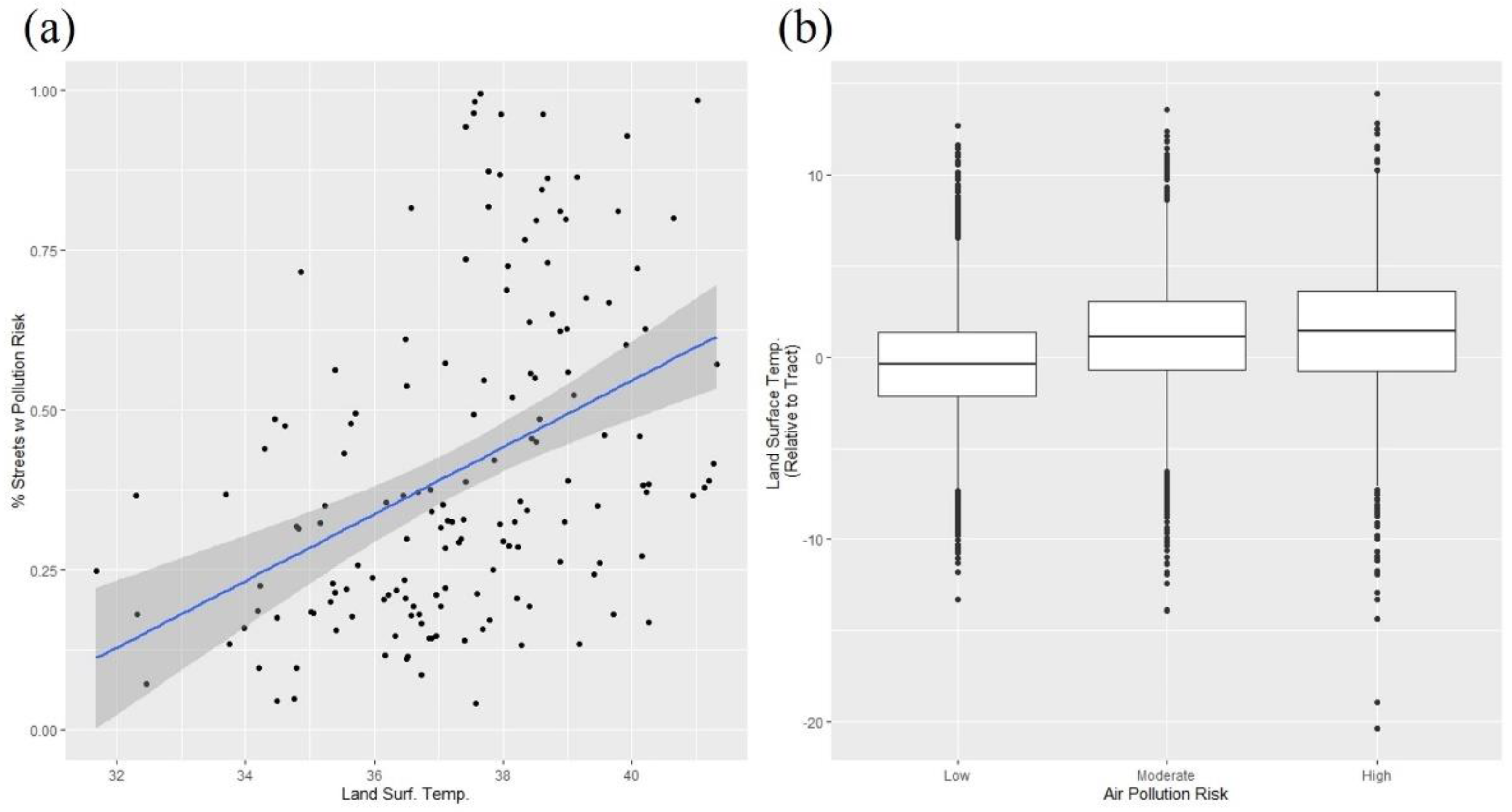
3.3. Overlaps in Hazards across and within Neighborhoods

An initial examination finds that there is a significant though moderate correlation of r = 0.41 (p < 0.001) between average temperature and the proportion of streets at risk for air pollution. This correlation is apparent in Figure 3a, though it is notable that there are many places high in one that are not high in the other. As we have noted that there are substantial variations between streets within the same neighborhood for each of these hazards, it is worth considering whether these within-neighborhood variations correlate across hazards.
Streets at moderate risk for air pollution were about 3 °F warmer than low-risk streets, and high-risk streets were an additional 0.6°F warmer on average (97.6 °F, 100.6 °F, and 101.2 °F). This relationship accounts for 10% of the variation in temperature (using an ANOVA with pollution risk level predicting LST; p < 0.001), which is equivalent to a correlation of 0.32, or just a bit lower than the correlation across tracts. However, the relationship weakens if we compare streets only to their neighbors (i.e., using the ANOVA to predict the LST of a street relative to the temperature of the census tract), with the correlation dropping to 0.24 (R2 = 0.06, p < 0.001). In fact, although low air pollution streets are somewhat cooler on average than their neighbors (−0.39 °F relative to the neighborhood average), moderate- and high-risk streets in the same neighborhood are practically identical to each other (1.16 °F and 1.21 °F relative to the neighborhood average, respectively).
If we categorize streets by whether they suffer from air pollution, above average heat, neither, or both, we see an interesting pattern. Streets that are cooler than the average temperature in their neighborhood have an almost perfectly 50% chance of being at-risk for air pollution, but streets that have above-average temperature have over a 70% chance of being at-risk for air pollution. This implies that factors that drive heat (e.g., impervious surfaces) tend to be accompanied by vehicles. Though that relationship is not as consistent in the other direction, it gives us a guide to places that suffer from both hazards.

4. Discussion

The findings demonstrate the presence of microspatial inequities in the distribution of extreme heat and air pollution in Boston, MA. Just under half of the variation in heat and approximately 75% of the variation in air pollution occurred within neighborhoods, indicating that individuals living only a few blocks away from each other might experience markedly different conditions in their daily lives. For instance, temperature differences between streets in the same census tract were as great as 20 °F. This can be clearly seen in Figure 1, where tracts vary considerably in their aggregate level of hazards but also in the range of environments occurring within them. These results run counter to traditional conceptions of geographic inequities, which assume that such disparities exist primarily between neighborhoods and are uncommon within neighborhoods (e.g., [15,16]); but they align well with the understanding of geophysical processes that are known to contribute to environmental hazards. We confirmed that these hyperlocal features of infrastructure and urban design were predominantly responsible not only for differences within neighborhoods but also between neighborhoods. That is, even where we see cross-neighborhood disparities in environmental hazards, they can largely be attributed to the types of streets comprising each.
Second, we see that the distributions of extreme heat and air pollution overlap in some areas but not consistently. The two hazards were moderately correlated across neighborhoods but only modestly correlated across the streets of a given neighborhood. For example, in the example neighborhood depicted in Figure 2, streets with high air pollution are not necessarily those with high temperature and vice versa. This again contrasts with neighborhood-centric models of inequity, which often theorize how a single overarching process can lead multiple negative conditions and outcomes to cluster together in certain locations [14,15,16,17,35]. It is worth noting, though, that attention to the geophysical processes underlying environmental hazards would predict the results we saw here. If two hazards arise from different infrastructural drivers then we would have no reason to expect that those hazards necessarily overlap with each other except to the extent that their drivers overlap. Indeed, the correlation that does exist between extreme heat and air pollution is likely attributable to high-pavement-low-canopy areas with high vehicular traffic. However, there are ways to have high traffic without low canopy cover (e.g., tree-lined parkways) and high pavement without high traffic (e.g., industrial zones). To our knowledge this is the first study to fully test the correlations between multiple hazards at these geographical scales.
The primary implication for sustainability and climate resilience is the need for more nuance in how we conceptualize spatial inequities. It is easy to rely on tropes about “high and low pollution” or “high and low heat” communities. Worse, we often fall back on simplistic definitions of “environmental justice communities”, which are defined by demographic indices of social vulnerability and rarely if ever differentiated by the hazards they do and do not experience [57,58]. The results here indicate that there is no single high-risk neighborhood for any environmental hazard, not to mention their combinations. Instead, each neighborhood has its unique landscape, wherein some streets have greater hazards and others less. From there, future research will need to further explore how these varied contexts impact public health and wellbeing given their combination and levels of hazards.
We conclude by exploring the technological and conceptual tools that we need to capitalize on our emergent understanding of the hyperlocal distribution of hazards. First, developing interventions and action plans for microspatial inequities will require detailed street-by-street—or even more granular—information for all neighborhoods. One might argue that the data presented here already begin do that, however Section 2 details the acknowledged limitations of these data. In fact, we believe this preliminary work demonstrates the need for higher spatial resolution in situ data, which could as a first step be used to verify whether or not the proxies we used here are sufficient to capture true variability and underlying drivers. These validated results could then (1) assess the benefit of field-deployed sensor networks as a complement to existing data repositories and (2) improve utility for and reliability in guiding action. In particular, deployed environmental sensor networks could be designed to reflect the contours of the local landscape, with more sensors in areas anticipated to be highly variable, and could uncover distinctive rhythms in hazards over the course of days and seasons that may otherwise be obscured by annual averages or even remotely sensed data. That said, the issue of cost remains and many communities may not have the resources to construct environmental sensor networks. Cost-efficient solutions might include the use of mobile sensors placed on vehicles, which have been used for both heat (e.g., [59]) and air pollution (e.g., [60]), or sparser networks that strategically capitalize on variations and consistencies in the landscape to still produce reliable estimates across space.
Environmental sensor networks are not silver bullets, however, capable of translating hazard maps into sustainability, climate resilience, and wellbeing for all. There are many possible ways that we might address microspatial inequities in hazard exposure, including modifications of infrastructure (e.g., the implementation of green infrastructure) and the organization of service delivery (e.g., the optimal placement of cooling centers during heat waves). That said, these cannot be top-down solutions. Instead, community members themselves are the best equipped to speak to what microspatial inequities mean for their daily lives and how they might want to see them alleviated. For instance, what if the introduction of more canopy cover on a hot street could result in less parking? Is that a tradeoff that the community prefers? Data from sensors must be incorporated into community conversations if such questions are to be explored and resolved. There are techniques for doing so, especially from the burgeoning field of participatory modeling, which develops shared representations that permit the merger of stakeholder perspectives and scientific data in the design and testing of solutions to complex community problems [61,62,63]. Such conversations may help solve the unanswered riddle of how sensor networks realize the promise of benefitting community and facilitate the development of science-driven, community-led solutions for locally-based sustainability and climate resilience.

Author Contributions

Conceptualization, D.T.O. and A.V.M.; methodology, D.T.O. and A.V.M.; formal analysis, D.T.O. and A.V.M.; writing—original draft preparation, D.T.O.; writing—review and editing, D.T.O. and A.V.M. All authors have read and agreed to the published version of the manuscript.

Funding

This research received support from the National Science Foundation’s Smart & Connected Communities program (award #2230036) and from the iSUPER Impact Engine at Northeastern University.

Institutional Review Board Statement

The work contained no data on human subjects and thus did not undergo IRB review.

Informed Consent Statement

Not applicable.

Data Availability Statement

Data will be published through the Boston Area Research Initiative’s Boston Data Portal, hosted by the Harvard Dataverse, before publication.

Acknowledgments

The authors thank their colleagues Moira Zellner and Michelle Laboy for regular conversations about the nature of microspatial inequities; Lucy Hutyra, Conor Gately, and Andrew Trlica for making the Urban Heat Island database and air pollution emissions data publicly available; and members of the Boston Area Research Initiative team who have maintained the Geographical Infrastructure over the years, most notably Alina Ristea, Saina Sheini, and Michael Zoorob.

Conflicts of Interest

The authors declare no conflict of interest.

References

  1. Chakraborty, J.; Collins, T.W.; Grineski, S.E. Exploring the Environmental Justice Implications of Hurricane Harvey Flooding in Greater Houston, Texas. Am. J. Public Health 2019, 109, 244–250. [Google Scholar] [CrossRef]
  2. Collins, T.W.; Grineski, S.E.; Chakraborty, J.; Flores, A. Environmental injustice and Hurricane Harvey: A household-level study of socially disparate flood exposures in Greater Houston, Texas, USA. Environ. Res. 2019, 179, 108772. [Google Scholar] [CrossRef]
  3. Browning, C.R.; Wallace, D.; Feinberg, S.L.; Cagney, K.A. Neighborhood Social Processes, Physical Conditions, and Disaster-Related Mortality: The Case of the 1995 Chicago Heat Wave. Am. Sociol. Rev. 2006, 71, 661–678. [Google Scholar] [CrossRef]
  4. Chang, L.-Y.; Foshee, V.A.; Reyes, H.L.M.; Ennett, S.T.; Halpern, C.T. Direct and Indirect Effects of Neighborhood Characteristics on the Perpetration of Dating Violence Across Adolescence. J. Youth Adolesc. 2015, 44, 727–744. [Google Scholar] [CrossRef]
  5. Harlan, S.L.; Declet-Barreto, J.H.; Stefanov, W.L.; Petitti, D.B. Neighborhood Effects on Heat Deaths: Social and Environmental Predictors of Vulnerability in Maricopa County, Arizona. Environ. Health Perspect. 2013, 121, 197–204. [Google Scholar] [CrossRef] [PubMed]
  6. Hoffman, J.S.; Shandas, V.; Pendleton, N. The Effects of Historical Housing Policies on Resident Exposure to Intra-Urban Heat: A Study of 108 US Urban Areas. Climate 2020, 8, 12. [Google Scholar] [CrossRef]
  7. Molina, L.T.; Molina, M.J.; Slott, R.S.; Kolb, C.E.; Gbor, P.K.; Meng, F.; Singh, R.B.; Galvez, O.; Sloan, J.J.; Anderson, W.P.; et al. Air quality in selected megacities. J. Air Waste Manag. 2004, 54, 1–73. [Google Scholar] [CrossRef]
  8. Gurjar, B.; Jain, A.; Sharma, A.; Agarwal, A.; Gupta, P.; Nagpure, A.; Lelieveld, J. Human health risks in megacities due to air pollution. Atmos. Environ. 2010, 44, 4606–4613. [Google Scholar] [CrossRef]
  9. Kumar, P.; Jain, S.; Gurjar, B.R.; Sharma, P.; Khare, M.; Morawska, L.; Britter, R. New directions: Can a “blue sky” return to Indian megacities. Atmos. Environ. 2013, 71, 198–201. [Google Scholar] [CrossRef]
  10. Catlett, C.E.; Beckman, P.H.; Sankaran, R.; Galvin, K.K. Array of things: A scientific research instrument in the public way. In Proceedings of the 2nd International Workshop on Science of Smart City Operations and Platforms Engineering, SCOPE’17, Pittsburgh, PA, USA, 18–21 April 2017; Association for Computing Machinery: New York, NY, USA, 2017. [Google Scholar]
  11. Jacob, R.L.; Catlett, C.; Beckman, P.H.; Sankaran, R. Early results from the array of things. In Proceedings of the 2017 AGU Fall Meeting, New Orleans, LA, USA, 11–15 December 2017; p. H41J-1599. [Google Scholar]
  12. Shusterman, A.A.; Teige, V.E.; Turner, A.J.; Newman, C.; Kim, J.; Cohen, R.C. The BErkeley Atmospheric CO2 Observation Network: Initial evaluation. Atmos. Meas. Technol. 2016, 16, 13449–13463. [Google Scholar]
  13. Polak, J. Mobile environmental sensor systems across a grid environment-the MESSAGE project. ERCIM News, 15 January 2007; pp. 33–34. [Google Scholar]
  14. Du Bois, W.E.B. The Philadelphia Negro: A Social Study; University of Pennsylvania Press: Philadelphia, PA, USA, 1899. [Google Scholar]
  15. Shaw, C.; McKay, H. Juvenile Delinquency and Urban Areas; University of Chicago Press: Chicago, IL, USA, 1942. [Google Scholar]
  16. Sampson, R.J. Great American City: Chicago and the Enduring Neighborhood Effect; University of Chicago Press: Chicago, IL, USA, 2012. [Google Scholar]
  17. Wilson, W.J. The Truly Disadvantaged: The Inner City, the Underclass, and Public Policy; University of Chicago Press: Chicago, IL, USA, 1987. [Google Scholar]
  18. David, W.; Eck John, E.; Braga Anthony, A.; Breanne, C.; Kate, B.; Gerben, B.; Charlotte, G.; Groff Elizabeth, R.; Julie, H.; Hinkle Joshua, C.; et al. Place Matters: Criminology for the Twenty-First Century; Cambridge University Press: Cambridge, UK, 2016. [Google Scholar]
  19. Mohai, P.; Pellow, D.N.; Roberts, J.T. Environmental justice. Annu. Rev. Environ. Resour. 2009, 34, 405–430. [Google Scholar] [CrossRef]
  20. Bullard, R.D.; Wright, B. (Eds.) Race, Place, and Environmental Justice after Hurricane Katrina; Westview Press: Philadelphia, PA, USA, 2009. [Google Scholar]
  21. Bullard, R.D. Dumping in Dixie: Race, Class and Environmental Quality; Westview Press: Boulder, CO, USA, 1994. [Google Scholar]
  22. Logan, J.R.; Molotch, H. Urban Fortunes: The Political Economy of Place; University of California Press: Berkeley, CA, USA, 1987. [Google Scholar]
  23. Trlica, A.; Hutyra, L.R.; Schaaf, C.L.; Erb, A.; Wang, J.A. Albedo, Land Cover, and Daytime Surface Temperature Variation Across an Urbanized Landscape. Earth’s Future 2017, 5, 1084–1101. [Google Scholar] [CrossRef]
  24. Oke, T.R. Classics in physical geography revisited—Sundborg A. 1951: Climatological studies in Uppsala with special regard to the termperature conditions in the urban are. Prog. Phys. Geogr. 1995, 19, 107–113. [Google Scholar] [CrossRef]
  25. Oke, T.R. Towards better scientific communication in urban climate. Theor. Appl. Clim. 2006, 84, 179–190. [Google Scholar] [CrossRef]
  26. Gartland, L. Heat Islands: Understanding and Mitigating Heat in Urban Areas; Earthscan: Washington, DC, USA, 2011. [Google Scholar]
  27. Huang, G.; Cadenasso, M.L. People, landscape, and urban heat island: Dynamics among neighborhood social conditions, land cover and surface temperatures. Landsc. Ecol. 2016, 31, 2507–2515. [Google Scholar] [CrossRef]
  28. Huang, G.; Zhou, W.; Cadenasso, M.L. Is everyone hot in the city? Spatial pattern of land surface temperatures, land cover and neighborhood socioeconomic characteristics in Baltimore City, MD. J. Environ. Manag. 2011, 92, 1753–1759. [Google Scholar] [CrossRef]
  29. Harlan, S.L.; Brazel, A.J.; Prashad, L.; Stefanov, W.L.; Larsen, L. Neighborhood microclimates and vulnerability to heat stress. Soc. Sci. Med. 2006, 63, 2847–2863. [Google Scholar] [CrossRef]
  30. Hart, M.A.; Sailor, D.J. Quantifying the influence of land-use and surface characteristics on spatial variability in the urban heat island. Theor. Appl. Climatol. 2009, 95, 397–406. [Google Scholar] [CrossRef]
  31. Kumar, P.; Fennell, P.; Britter, R. Effect of wind direction and speed on the dispersion of nucleation and accumulation mode particles in an urban street canyon. Sci. Total Environ. 2008, 402, 82–94. [Google Scholar] [CrossRef]
  32. Xie, X.; Liu, C.-H.; Leung, D.Y. Impact of building facades and ground heating on wind flow and pollutant transport in street canyons. Atmos. Environ. 2007, 41, 9030–9049. [Google Scholar] [CrossRef]
  33. Soulhac, L.; Perkins, R.J.; Salizzoni, P. Flow in a Street Canyon for any External Wind Direction. Bound.-Layer Meteorol. 2008, 126, 365–388. [Google Scholar] [CrossRef]
  34. Gromke, C.C.; Ruck, B. Pollutant Concentrations in Street Canyons of Different Aspect Ratio with Avenues of Trees for Various Wind Directions. Bound.-Layer Meteorol. 2012, 144, 41–64. [Google Scholar] [CrossRef]
  35. Chetty, R.; Hendren, N. The Impacts of Neighborhoods on Intergenerational Mobility II: County-Level Estimates*. Q. J. Econ. 2018, 133, 1163–1228. [Google Scholar] [CrossRef]
  36. Cutter, S. Race, class and environmental justice. Prog. Hum. Geogr. 1995, 19, 111–122. [Google Scholar] [CrossRef]
  37. Maantay, J. Asthma and air pollution in the Bronx: Methodological and data considerations in using GIS for environmental justice and health research. Health Place 2007, 13, 32–56. [Google Scholar] [CrossRef] [PubMed]
  38. Chakraborty, J.; Schweitzer, L.A.; Forkenbrock, D.J. Using GIS to Assess the Environmental Justice Consequences of Transportation System Changes. Trans. GIS 1999, 3, 239–258. [Google Scholar] [CrossRef]
  39. Scientists, U.o.C. Inequitable Exposure to Air Pollution from Vehicles in Massachusetts; Union of Concerned Scientists: Cambridge, MA, USA, 2019. [Google Scholar]
  40. Clark, L.P.; Millet, D.B.; Marshall, J.D. Changes in Transportation-Related Air Pollution Exposures by Race-Ethnicity and Socioeconomic Status: Outdoor Nitrogen Dioxide in the United States in 2000 and 2010. Environ. Health Perspect. 2017, 125, 097012. [Google Scholar] [CrossRef]
  41. Sabrin, S.; Karimi, M.; Nazari, R. Developing Vulnerability Index to Quantify Urban Heat Islands Effects Coupled with Air Pollution: A Case Study of Camden, NJ. ISPRS Int. J. Geo-Inf. 2020, 9, 349. [Google Scholar] [CrossRef]
  42. Jenerette, G.D.; Harlan, S.L.; Brazel, A.; Jones, N.; Larsen, L.; Stefanov, W.L. Regional relationships between surface temperature, vegetation, and human settlement in a rapidly urbanizing ecosystem. Landsc. Ecol. 2007, 22, 353–365. [Google Scholar] [CrossRef]
  43. Rosenzweig, C.; Solecki, W.; Parshall, L.; Gaffin, S.; Lynn, B.; Goldberg, R.; Cox, J.; Hodges, S. Mitigating New York City’s Heat Island with Urban Forestry, Living Roofs, and Light Surfaces. In Proceedings of the Sixth Symposium on the Urban Environment, Capri, Italy, 18–20 May 2022; American Meteorological Society: Atlanta, GA, USA, 2006. [Google Scholar]
  44. Bullard, R.D. (Ed.) Confronting Environmental Racism: Voices from the Grassroots; South End Press: Cambridge, MA, USA, 1993. [Google Scholar]
  45. O’Brien, D.T.; Gridley, B.; Trlica, A.; Wang, J.A.; Shrivastava, A. Urban heat islets: Street segments, land surface temperatures and medical emergencies during heat advisories. Am. J. Public Health 2020, 110, 994–1001. [Google Scholar] [CrossRef]
  46. Gately, C.K.; Hutyra, L.R.; Peterson, S.; Wing, I.S. Urban emissions hotspots: Quantifying vehicle congestion and air pollution using mobile phone GPS data. Environ. Pollut. 2017, 229, 496–504. [Google Scholar] [CrossRef] [PubMed]
  47. Trlica, A. Urban Land Cover and Urban Heat Island Effect Database; Boston Area Research Initiative: Boston, MA, USA, 2017. [Google Scholar]
  48. Gately, C.; Hutyra, L.; Peterson, S.; Sue Wing, I. High Resolution Vehicle Air Pollutant Emissions for Eastern Massachusetts; Harvard Dataverse: Cambridge, MA, USA, 2017. [Google Scholar]
  49. O’Brien, D.T.; Phillips, N.; de Benedictis-Kessner, J.; Shields, M.; Sheini, S. 2018 Geographical Infrastructure for the City of Boston; Boston Area Research Initiative: Boston, MA, USA, 2018. [Google Scholar]
  50. Zhu, Z.; Woodcock, C.E. Object-based cloud and cloud shadow detection in Landsat imagery. Remote Sens. Environ. 2012, 118, 83–94. [Google Scholar] [CrossRef]
  51. Barsi, J.A.; Schott, J.R.; Palluconi, F.D.; Hook, S.J. Validation of a web-based atmospheric correction tool for single thermal band instruments. In Proceedings of the SPIE 5882, Earth Observing Systems X, San Diego, CA, USA, 22 August 2005. [Google Scholar]
  52. Melaas, E.K.; Wang, J.A.; Miller, D.L.; Friedl, M.A. Interactions between urban vegetation and surface urban heat islands: A case study in the Boston metropolitan region. Environ. Res. Lett. 2016, 11, 054020. [Google Scholar] [CrossRef]
  53. Shuai, Y.; Masek, J.G.; Gao, F.; Schaaf, C.B. An algorithm for the retrieval of 30-m snow-free albedo from Landsat surface reflectance and MODIS BRDF. Remote Sens. Environ. 2011, 115, 2204–2216. [Google Scholar] [CrossRef]
  54. Homer, C.; Dewitz, J.; Yang, L.; Jin, S.; Danielson, P.; Xian, G.; Coulston, J.; Herold, N.; Wickham, J.; Megown, K. Completion of the 2011 National Land Cover Database for the coterminous United States-Representing a decade of land cover change infrmation. Photogramm. Eng. Remote Sens. 2015, 81, 345–354. [Google Scholar]
  55. Nahlik, M.J.; Chester, M.V.; Pincetl, S.S.; Eisenman, D.; Sivaraman, D.; English, P. Building thermal performance, extreme heat, and climate change. J. Infrastruct. Syst. 2017, 23, 04016043. [Google Scholar] [CrossRef]
  56. Bates, D.; Maechler, M.; Bolker, B.; Walker, S.; Christensen, R.H.B.; Singmann, H. Linear Mixed-Effects Models Using ‘Eigen’ and S4. 2017. Available online: https://cran.r-project.org/web/packages/lme4/index.html (accessed on 15 November 2022).
  57. Spielman, S.E.; Tuccillo, J.; Folch, D.C.; Schweikert, A.; Davies, R.; Wood, N.; Tate, E. Evaluating social vulnerability indicators: Criteria and their application to the Social Vulnerability Index. Nat. Hazards 2020, 100, 417–436. [Google Scholar] [CrossRef]
  58. Flanagan, B.E.; Gregory, E.W.; Hallisey, E.J.; Heitgerd, J.L.; Lewis, B. A social vulnerability index for disaster management. J. Homel. Secur. Emerg. Manag. 2011, 8, 3. [Google Scholar] [CrossRef]
  59. Benson, S.; Sittenfeld, D.F.; Shandas, V.; Hoffman, J.S.; Baur, K.; Harrington, S.; Cavalier, D. Wicked hot Boston: Connecting citizen science to extreme heat events through urban heat mapping and ISeeChange. In Proceedings of the 100th American Meteorological Society Annual Meeting, Boston, MA, USA, 12–16 January 2020. [Google Scholar]
  60. Buehler, C.; Xiong, F.; Zamora, M.L.; Skog, K.M.; Kohrman-Glaser, J.; Colton, S.; McNamara, M.; Ryan, K.; Redlich, C.; Bartos, M.; et al. Stationary and portable multipollutant monitors for high spatiotemporal resolution air quality studies including online calibration. Atmos. Meas. Technol. Discuss. 2020, 14, 995–1013. [Google Scholar] [CrossRef]
  61. Zellner, M.; García, G.A.; Bert, F.; Massey, D.; Nosetto, M. Exploring reciprocal interactions between groundwater and land cover decisions in flat agricultural areas and variable climate. Environ. Model. Softw. 2020, 126, 104641. [Google Scholar] [CrossRef]
  62. Gray, S.; Voinov, A.; Paolisso, M.; Jordan, R.; BenDor, T.; Bommel, P.; Glynn, P.; Hedelin, B.; Hubacek, K.; Introne, J.; et al. Purpose, processes, partnerships, and products: Four Ps to advance participatory socio-environmental modeling. Ecol. Appl. 2018, 28, 46–61. [Google Scholar] [CrossRef] [PubMed]
  63. Sterling, E.J.; Zellner, M.; Jenni, K.E.; Leong, K.; Glynn, P.D.; Bendor, T.K.; Bommel, P.; Hubacek, K.; Jetter, A.J.; Jordan, R.; et al. Try, try again: Lessons learned from success and failure in participatory modeling. Elem. Sci. Anthr. 2019, 7, 9. [Google Scholar] [CrossRef] [Green Version]
Figure 1. Maps of the distribution of hazards across tracts reveal large amounts of variability across neighborhoods in (a) heat and (b) air pollution, but also large amounts of variability within neighborhoods, as measured by (c) difference in temperature between the warmest and coolest streets and (d) the diversity of at-risk and low-risk streets for air pollution (calculated with a Herfindahl index, 1 − p2 − (1 − p)2). Note: Variability only represented for tracts with 20 or more streets to avoid outliers.
Sustainability 15 02984 g001
Figure 2. Depictions of within-neighborhood variability in hazards alongside the distribution of common drivers in a single census tract in Boston. (a) Land surface temperature, (b) air pollution risk, (c) canopy coverage, and (d) classification as a main street.
Sustainability 15 02984 g002
Figure 3. The correlation between land surface temperature and air pollution risk is (a) moderately strong at the census tract level (R2 = 0.17; represented by trendline) but (b) weak between street segments in the same tract (R2 = 0.06).
Sustainability 15 02984 g003
Table 1. Descriptive statistics for streets in Boston with measures of heat and air pollution and the containing census tracts.
w/Msr. of Heatw/Msr. of Poll. a
Mean (SD or Range)
or Count (%)
Mean (SD or Range)
or Count (%)
Street Segment Features
Main Streetb9004 (37%)3591 (28%)
Dead End1232 (5%)1131 (9%)
Predominant Zoning
 No Parcels10,785 (44%)
 Three-Family Residential with Assorted Other Uses1843 (7%)1840 (14%)
 Mix of Two-Family and Single-Family Residential2530 (10%)2523 (19%)
 Commercial2375 (10%)2225 (17%)
 Single-Family Residential Only3333 (14%)3307 (26%)
 Exempt c1533 (6%)917 (7%)
 Condominiums1594 (6%)1578 (12%)
 Mixed-Use Commercial586 (2%)564 (4%)
Land Surface Temperature98.6 °F (5.5 °F)98.8 °F (4.8 °F)
Canopy Cover0.10 (0.14)0.11 (0.12)
Impervious Surface Cover0.77 (0.23)0.76 (0.20)
Albedo0.13 (0.02)0.12 (0.02)
Air Pollution Classificationd
 Low-Risk7912 (61%)7918 (61%)
 Medium-Risk3484 (27%)3491 (27%)
 High-Risk1540 (12%)1545 (12%)
n = 24,579n = 12,954
Census Tract Features
Pop. Density25,336 ppl/mi2 (18,159 ppl/mi2)25,478 ppl/mi2 (18,110 ppl/mi2)
Predominant Usage
 Downtown12 (7%)12 (7%)
 Industrial/Institutional31 (17%)31 (17%)
 Park14 (8%)13 (8%)
 Residential121 (68%)121 (68%)
n = 178n = 177
a—Estimates of pollution limited to streets with at least one parcel with a stated number of floors in tax assessments. See Methods for more detail. b—As determined by the Commonwealth of Massachusetts’ MassGIS, which categorizes streets according to their width and thoroughfare status. See Methods for more detail. c—Buildings owned by government, and non-profits are tax exempt. In addition, Chapter 121A establishes subsidized housing as tax exempt. d—18 street segments had estimates for air pollution but no values from the urban heat island database, making for 12,936 segments with measures on both.
Table 2. Parameter estimates from multilevel models predicting the distribution of land surface temperature and air pollution risk based on street- and tract-level features.
Land Surf. Temp.Moderate- or High-Risk for Air Pollution? (0/1)
Beta (SE)Beta (SE)Beta (SE)Odds RatioBeta (SE)Odds Ratio
Street-Level Features
Canopy Covera−14.95 *** (0.18)−14.72 *** (0.18)
Imperv. Surf. Covera6.70 *** (0.13)6.54 *** (0.13)
Albedoa−17.32 *** (1.15)−17.28 *** (1.15)
Main3.68 *** (0.08)39.653.68 *** (0.08)39.65
Dead End0.12 (0.09)1.130.12 (0.09)1.13
Predominant Zoningb
 Three-Family Res.0.69 *** (0.10)1.990.67 *** (0.10)1.95
 Two- and Single-Family Res.0.23 ** (0.09)1.260.22 * (0.09)1.25
−0.09
 Commercial1.32 *** (0.10)3.741.29 *** (0.10)3.63
 Exempt0.88 *** (0.13)2.410.85 *** (0.13)2.34
 Condos0.61 *** (0.10)1.840.58 *** (0.10)1.79
 Mixed-Use1.75 *** (0.17)5.751.68 *** (0.17)5.37
Tract-Level Features
Canopy Covera−6.67 *** (1.34)
Imperv. Surf. Covera3.83 *** (1.03)
Albedoa−10.11 (9.91)
Population Densityc0.21 (0.13)1.23
Predominant Usaged
 Downtown1.37 *** (0.39)3.94
 Industrial/Institutional0.27 (0.24)1.31
 Park0.24 (0.46)1.27
 Street-Level R20.40.41ee
 Tract-Level R20.740.840.140.24
 Streets/Tracts f24,523/17512,721/155
*—p < 0.05, **—p < 0.01, ***—p < 0.001. a—Proportion measured from 0–1. b—Reference category of predominantly single-family zoning (see Table 1 for more). c—Log-transformed to account for outliers. d—Reference category of predominantly residential usage. e—Not possible to calculate for binomial model. f—Limited to street segments with all measures in census tracts with at least 20 street segments.
Disclaimer/Publisher’s Note: The statements, opinions and data contained in all publications are solely those of the individual author(s) and contributor(s) and not of MDPI and/or the editor(s). MDPI and/or the editor(s) disclaim responsibility for any injury to people or property resulting from any ideas, methods, instructions or products referred to in the content.

