Article

Mapping and Characterizing Eelgrass Meadows Using UAV Imagery in Placentia Bay and Trinity Bay, Newfoundland and Labrador, Canada

1
Department of Geography, Memorial University of Newfoundland, St. John’s, NL A1B 3X9, Canada
2
Institut de Recherche pour le Développement, Espace-Dev (IRD, U. Montpellier, U. Réunion, U. Guyane, U. Perpignan Via Domitia, U. Nouvelle-Calédonie), 34090 Montpellier, France
3
School of Ocean Technology, Fisheries and Marine Institute of Memorial University of Newfoundland, St. John’s, NL A1C 5R3, Canada
4
Centre for Fisheries Ecosystems Research, Fisheries and Marine Institute of Memorial University of Newfoundland, St. John’s, NL A1C 5R3, Canada
5
Institute of Marine Research, 5005 Bergen, Norway
6
Department of Biology, Memorial University of Newfoundland, St. John’s, NL A1C 5R3, Canada
*
Author to whom correspondence should be addressed.
Sustainability 2024, 16(8), 3471; https://doi.org/10.3390/su16083471
Submission received: 19 February 2024 / Revised: 14 April 2024 / Accepted: 16 April 2024 / Published: 21 April 2024
(This article belongs to the Special Issue Ecology, Biodiversity and Conservation in Seagrass Ecosystems)

Abstract

:
Sustainable coastal social–ecological systems rely on healthy ecosystems known to provide benefits to both nature and people. A key ecosystem found globally is seagrass, for which maps at a scale relevant to inform conservation and management efforts are often missing. Eelgrass (Zostera marina), a species of seagrass found throughout the northern hemisphere, has been declining in Placentia Bay, an ecologically and biologically significant area of Canada’s east coast subject to an increasing human impact. This research provides baseline information on the distribution of eelgrass meadows and their anthropogenic stressors at seven sites of Placentia Bay and three sites of the adjacent Trinity Bay, on the island of Newfoundland. High-resolution maps of eelgrass meadows were created by combining ground-truth underwater videos with unmanned aerial vehicle imagery classified with an object-based image analysis approach. Visual analyses of the imagery and underwater videos were conducted to characterize sites based on the presence of physical disturbances and the semi-quantitative cover of epiphytes, an indication of nutrient enrichment. A total eelgrass area of ~1 km2 was mapped across the 10 sites, with an overall map accuracy of over 80% for 8 of the 10 sites. Results indicated minimum pressures of physical disturbance and eutrophication affecting eelgrass in the region, likely due to the small population size of the communities near the eelgrass meadows. These baseline data will promote the sustainability of potential future coastal development in the region by facilitating the future monitoring and conservation of eelgrass ecosystems.

Graphical Abstract

1. Introduction

Seagrasses are marine plants that grow along the shorelines of all continents, except Antarctica, forming highly productive ecosystems that support a wide diversity of marine organisms, including invertebrates, fishes, reptiles, mammals, and waterfowl [1]. Seagrasses are considered among the most valuable ecosystems globally [2]. They provide key ecosystem services in coastal regions, supporting fisheries [3,4], protecting from coastal erosion [5], and acting as a sink for carbon [6,7]. Seagrasses are considered biological sentinels [8] and have been adopted as bioindicators for numerous marine ecosystem health monitoring programs [9,10,11,12].
Seagrasses, however, are threatened by a variety of anthropogenic stressors, including eutrophication, coastal development, sea level rise, physical disturbances (e.g., propeller scarring, trawling, or anchor damage), and increased water turbidity [13]. As a result, they were found to decline globally at an approximate rate of 1.5% yr−1 [14]. While seagrass has been shown to recover following management efforts, such as improving water quality [15,16], seagrass ecosystems are often impacted by multiple stressors [13]. For instance, Krause-Jensen et al. [17] assessed that the seagrass of the Western Baltic Sea, following the mitigation of eutrophication, did not return to its historic levels due to the additional impact of bottom trawling and to the increased water temperature. Sustainable approaches to coastal management, therefore, require to simultaneously address the multiple stressors of seagrass ecosystems.
One of the key challenges to monitor and consider seagrass ecosystems in sustainable coastal management is a lack of baseline information on seagrass distribution [18,19]. For instance, in Canada, where eelgrass (Zostera marina (L.)) has been documented on all three coasts, numerous meadows remain to be mapped and their extent quantified [18,20]. In addition to the need to map seagrass, threats to these ecosystems should be better understood at a local scale to effectively target management efforts [19].
On Canada’s east coast, eelgrass is the dominant seagrass species and is designated an ecologically significant species [21]. The eelgrass of Placentia Bay in the Province of Newfoundland and Labrador is in decline [22]. A study of 17 sites in Placentia Bay conducted in 2012 found the average eelgrass percent cover to be half the cover observed in 1998 [22]. These declines have been largely attributed to the European green crab (Carcinus maenas; Linnaeus, 1758), an invasive species that was first observed in this region in 2007 [23], which uproot eelgrass while burrowing or foraging in soft sediments [22,24]. In contrast, eelgrass in nearby coastal areas of the island of Newfoundland not colonized by green crabs has been reported to be expanding [25]. Previous eelgrass mapping efforts on the island of Newfoundland, however, consisted mostly of point observations indicating where eelgrass is present or is likely to occur [26], but provided limited value in terms of baseline data to monitor temporal changes in eelgrass extent (but see [27]).
While the impact of green crab on eelgrass has been documented in Placentia Bay, the role of other anthropogenic stressors, such as the increasing maritime traffic and the development of large-scale salmon aquaculture [28,29], has not been investigated. Furthermore, many of the communities along the coast of Placentia Bay do not have modern forms of wastewater management, and sewage has been reported to accumulate in some sheltered areas of Placentia Bay [28,30]. Excess nutrients from aquaculture and wastewater can cause eutrophication, reducing light availability for seagrass [31,32]. Finally, there are mooring areas with varying degrees of boating intensity, ranging from single docks used for recreational boating to harbours for small fishing vessels. Boating-related activities have been shown to have a negative impact on seagrasses, with damages caused by propeller scars [33,34], mooring scours [35,36], dock shading [37,38], and anchoring [39,40]. While the individual disturbances caused by boating-related activities are typically small, an accumulation of these disturbances over a larger region may be substantial (e.g., [36]).
This study provides baseline data on the distribution of eelgrass in a region where eelgrass is thought to be declining but where there has been limited quantification of eelgrass extent or the prevalence of common anthropogenic stressors. The study combined the use of an unmanned aerial vehicle (UAV) that helped produce very high-resolution imagery of each study site and ground-truth underwater imagery, allowing high-resolution seagrass maps to be created. The objectives of this study were (1) to delineate the spatial extent of seven eelgrass meadows in Placentia Bay and three eelgrass meadows in Trinity Bay, and (2) to provide local context to the occurrence and impact of eutrophication and physical disturbance to eelgrass meadows at these sites.

2. Materials and Methods

2.1. Study Sites

Study sites were selected based on previous knowledge of eelgrass presence, as observed by Matheson et al. [22] and Rao et al. [26]. All sites consisted of subtidal eelgrass meadows. To help understand the prevalence of anthropogenic stressors, five sites were selected in areas with limited human development in the surrounding area, while five other sites were selected in areas experiencing greater levels of human activities—where anthropogenic disturbances (i.e., anchor damage, propeller scaring, and dock shading) or nutrient pollution could be expected (Figure 1). Sites with higher human presence were along the shoreline of a community where drainages or docking infrastructure for motorboats were present. Sites with lower human presence were selected to have minimal presence of infrastructure except for roads to allow for vehicle access. Seven of those study sites were selected in Placentia Bay, while three sites were selected in Trinity Bay (Figure 1), a nearby coastal area outside the invasion range of the European green crab.

2.2. Aerial Image Collection and Processing

Aerial imagery was collected using a Da-Jiang Innovations (DJI) Mavic 2 Professional UAV from August to September 2020, during the peak eelgrass biomass period [41]. UAV image collection was conducted when the sun’s angle was less than 40° and, when possible, cloud cover was <10% or >90%, specifically targeting overcast or clear sky days, following the recommendations made by Nahirnick et al. [42]. Due to safe operating guidelines for the UAV, image collection was conducted on days when wind gust speeds were below 30 km/h, which also resulted in limited sea surface roughness in the images. DJI’s Ground Station Pro app v.2.0.12 was used to plan and conduct the UAV surveys. The survey was designed to obtain nadir images with a forward and lateral overlap of 80% obtained at an altitude of 120 m, resulting in images at about 2.8 cm/pixel resolution. Images were captured at a flight speed of 5 m/s using the hover and capture flight mode. For georeferencing the orthomosaics during image processing, the positions of at least seven Ground Control Points (GCPs), distributed as evenly as possible throughout each field site on dry land, were collected with a Garmin eTrex 20x (~3 m accuracy) global positioning system (GPS), using the waypoint averaging function until a sample confidence of 100% was achieved.
Agisoft Metashape Professional v.1.6.1 [43] was used to create orthomosaics of the UAV imagery. All land and anthropogenic features (docks, boats, etc.) were manually masked from each site in ESRI ArcGIS 10.7 [44], and the orthomosaics were resampled to a spatial resolution of 25 cm to improve the processing time of image classification.

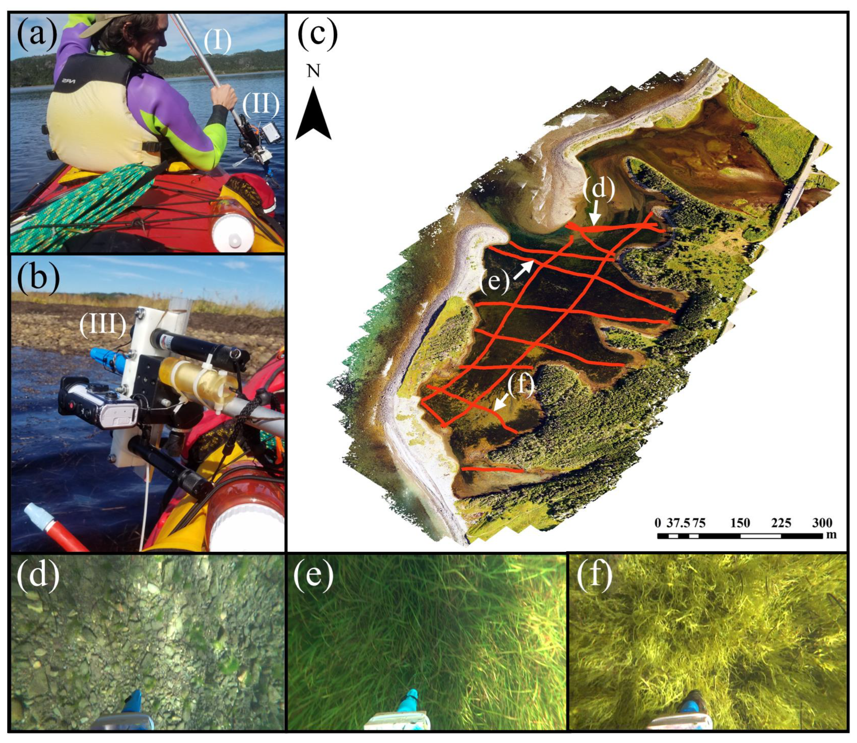
2.3. Ground-Truth Data

Based on visual inspection of the UAV orthomosaics of each study site, underwater video collection was planned for a later day such that video observations were distributed throughout the entire study areas, allowing the collection of images over as many cover types/habitats as possible (Figure 2). The goal being to conduct a supervised classification of an aerial image, this sampling did not aim to cover the entire area but to provide sample videos representative of the underwater landscape. Sampling generally involved the crossing in straight line of the water body from shore to shore using a kayak. Ground-truth data collection was conducted within 11 to 54 ( x ¯ = 35.6) days of aerial image collection. Underwater videos were collected using a Sony FDR-X3000 ActionCam. The camera was operated in an underwater housing from a slow-moving 2-person kayak, while the Garmin eTrex 20x GPS recorded the position of the camera operator. The time stamps of the GPS coordinates were matched in post-processing with the video data by recording a few seconds of a digital clock synchronized with the GPS time at the start or end of each video. Improving on the limitations identified by Nahirnick et al. [45] for collecting ground-truth data with a camera attached to the bottom of a kayak, the underwater camera was affixed to an Unger 8–16 ft aluminum telescopic pole (Figure 2). The pole height was adjusted by the camera operator to position the camera near the target features directly under the kayak.
The underwater videos were used to generate a series of training data points for each field site. Transects were buffered at 3 m in ArcGIS, corresponding to the approximate average horizontal accuracy of the GPS, and observations were made at least every 5 s along the underwater video transects by creating point features within the buffer. Point features were created when a cover type could be identified in both the underwater video and the orthomosaic. The classification scheme for each site varied depending on the cover types present at each site. Each classification scheme started with two classes: sediment and eelgrass. Additional classes (i.e., shadows, optically deep water, benthic periphytic brown algae, benthic periphytic green algae, spume, detritus, turbid water, and shells) were added depending on their presence in the transect observations.

2.4. OBIA and Classification

Object-based image analysis (OBIA) is commonly employed for the accurate classification of high-resolution imagery through the process of image segmentation [46]. The R statistical software (v3.6.1) [47] package SegOptim 0.2.2 [48] was used for image segmentation and classification. SegOptim uses a genetic algorithm, a machine learning algorithm that emulates the process of natural selection, to determine the optimal parameter settings for the segmentation algorithm, and can interface with six third-party software to conduct image segmentation. SegOptim’s segmentation_ArcGIS_Mshift function was used to conduct image segmentation due to the comparable performance of the algorithm to others available in SegOptim [48] and the wide use of ArcGIS as a GIS software. The mean shift segmentation method used by this function [49] uses three parameters: spatial detail, spectral detail, and minimum segment size. To improve the efficiency of the genetic algorithm, it is important to constrain the parameter space to avoid poor solutions and to improve computation time [48]. Details on delineating the parameter space are provided in the Supplementary Materials.
Image classification was conducted using the mean and standard deviation of RGB values for the image segments [50,51,52]. The classification of the image segments was conducted using SegOptim’s random forest classifier with the default parameters (ntree = 250, mtry = 2). The random forest classifier was selected for its performance compared to other machine learning classifiers [53] and was frequently the best preforming classification algorithm for use in SegOptim [48].
For some orthomosaics, the segmentation parameters were manually specified because SegOptim’s genetic algorithm systematically under-segmented the images. Under-segmentation is an issue in OBIA that occurs when image objects encompass multiple target features (e.g., a patch of eelgrass and a patch of algae are in one image object when they should be two separate objects). The maximum amount of detail (i.e., maximum spatial and spectral detail, with a minimum segment size of one pixel) was required to produce a segmentation that was not under-segmenting. In these instances, the classification was conducted using the mean RGB values for the image segments alone, as a standard deviation cannot be calculated for image segments with one pixel.
Training and validation for the random forest classifier were conducted using five-fold cross-validation. Millard and Richardson [54] identified that training data for use in random forest classification should be sufficiently large, have a random distribution or class proportions that reflect the actual proportions of the classes on the landscape, and minimal spatial autocorrelation. A dataset with these attributes improves classification results and will reduce model overfitting [54]. To produce a dataset with these attributes, 300 observations for each site was deemed sufficiently large. To avoid model overfitting, the 300 data points consisted of a combination of randomly sampled transect observations and randomly distributed photo interpretation points. Such a combination of ground-truth data and photo interpretation points has been previously used in UAV mapping research (e.g., [51,55]). Indeed, such high-resolution images were shown to be interpreted accurately by trained photo interpreters, removing the reliance on field observations [50]. A random sample of 100 transect observations, separated by at least 5 m, was taken from the transect data points in R. In ArcGIS, 200 points, separated by at least 5 m, were randomly generated within the study boundary of each site and outside of the 3 m video transect buffers. Photo interpretation points were assigned a class corresponding to the 25 cm resolution orthomosaics. The 2.8 cm resolution images were occasionally referenced during this process to aid with photo interpretation. These two datasets were merged to create a file of observation presences containing 100 transect and 200 photo interpretation observations. A file of observation absences was generated from cells in a grid, with a 5 m cell size, that did not contain an observation. The presence and absence datasets were merged and spatial autocorrelation between observation presence and absence was assessed throughout the study site using a series of 10 global Moran’s I tests [56], with incrementally increasing threshold distances. Ten threshold distances were used to assess spatial autocorrelation across a range of scales. Threshold distances for the Moran’s I tests started at the minimum distance so that each observation had at least one neighbor, followed by 10 m and increasing increments of 5 m up to 50 m. If the distribution of the observations exhibited significant clustering or dispersion (p-value < 0.05) at any of these distance thresholds, a new dataset was generated, and the process was iterated. If subsequent resamples exhibited significant clustering or dispersion, the proportion of transect data in the dataset was reduced by increments of 25 (i.e., 75 randomly sampled transect observations and 225 randomly distributed photo interpretation points), and the process was iterated until a dataset was produced that had a random distribution at all threshold distances.

2.5. Classification Accuracy

Classification accuracy was assessed using SegOptim by calculating Cohen’s Kappa coefficient, overall accuracy, eelgrass class ‘producer’s accuracy’, and eelgrass class ‘user’s accuracy’ (hereafter called accuracy metrics). Kappa values were interpreted following the agreement categories outlined by Sim and Wright [57] (≤0 = poor; 0.1–0.20 = slight; 0.21–0.40 = fair; 0.41–0.60 = moderate; 0.61–0.80 = substantial; and 0.81–1.0 = almost perfect). Overall accuracy is the percent of correctly classified image objects out of the total sample. Eelgrass class producer’s accuracy is the commission error, or the accuracy of how often the eelgrass observations are correctly classified on the map. Eelgrass class user’s accuracy is the omission error, or the accuracy of how often eelgrass areas classified in the map will be present on the ground.
The accuracy of the maps was assessed using 5-fold cross-validation. To increase the likelihood of generating a permutation with an observation in each fold, additional observations were added via photo interpretation to any class that had fewer than 10 observations until 10 observations were achieved. Accuracy metrics were calculated for each fold when it was acting as the validation sample. The final accuracy metrics for each site were obtained from the confusion matrices for each fold by calculating the mean and standard deviation of the accuracy metrics.

2.6. Presence of Anthropogenic Stressors

A semi-quantitative cover of epiphytes was estimated at each site, as an indication of nutrient enrichment [58], and the occurrence and nature of physical disturbance was recorded. At sites with a proliferation of epiphytes, the semi-quantitative cover of epiphytes was visually assessed using the underwater videos. The percent of eelgrass surface in the field of view covered by epiphytes was visually estimated from the videos and classified using 6 classes (0%, 1–20%, 21–40%, 41–60%, 61–80%, and 81–100%) (Figure S1). The duration of video time for each cover category was recorded and the proportion of video length for each cover category was calculated.
The nature of physical disturbances was determined using a visual inspection of the UAV imagery. During field visits, when time allowed, underwater video was collected to ground-truth potential anthropogenic disturbances identified in the UAV imagery. The area of disturbance was estimated using ArcGIS by manually delineating disturbances observed in the orthomosaics and using the ‘Calculate Geometry’ tool to calculate the area of each disturbance. To calculate the percent area of eelgrass affected by anthropogenic disturbance, the total disturbance area was divided by the total area of eelgrass mapped across the ten study sites.

3. Results

3.1. Eelgrass Distribution

Maps delineating the distribution of eelgrass at each of the 10 study sites were generated (Figure 3 and Figures S2–S11). Individual study sites ranged from 0.1747 km2 to 0.3631 km2 in size. The total eelgrass extent at those 10 sites was estimated to be 1.073 km2, with a mean and median eelgrass area of 0.1073 km2 and 0.0801 km2, respectively, across the 10 sites. The largest eelgrass meadow was observed in western Placentia Southeast Arm (Figure 3e), with 0.3331 km2 of eelgrass. The smallest eelgrass meadow was observed in Glennons Cove Pond (Figure 3f), with 0.0013 km2 of eelgrass.

3.2. Map Accuracy Assessment

The mean and standard deviation of the classification accuracy assessments metrics from the five-fold cross-validation are presented in Table 1. The confusion matrix for each site is provided in Tables S1–S10, with Kappa values ranging from 0.22 to 0.81. Western Placentia Southeast Arm and Placentia Swans had “slight” and “fair” agreement levels, respectively. Placentia Swans (Figure 3d) was the worst preforming classification, ranking poorly across all accuracy assessment metrics. While western Placentia Southeast Arm had the lowest average Kappa value, the overall accuracy, eelgrass class producer’s accuracy, and eelgrass class user’s accuracy had high average values of 86.3%, 99.2%, and 87.5%, respectively. The other eight sites showed a “substantial” or better level of agreement, with Great Barasway Pond (Figure 3c) producing the most accurate classification. The average overall accuracy values ranged from 69.7% to 89.3%.
The average eelgrass class producer’s accuracy ranged from 23.3% to 99.2%, and the average eelgrass class user’s accuracy ranged from 48.8% to 95.1%. Sites with smaller eelgrass area generally had the lowest eelgrass class accuracy metrics; the Placentia Swans site was an exception to this, with a moderate amount of eelgrass cover and a poor classification accuracy.

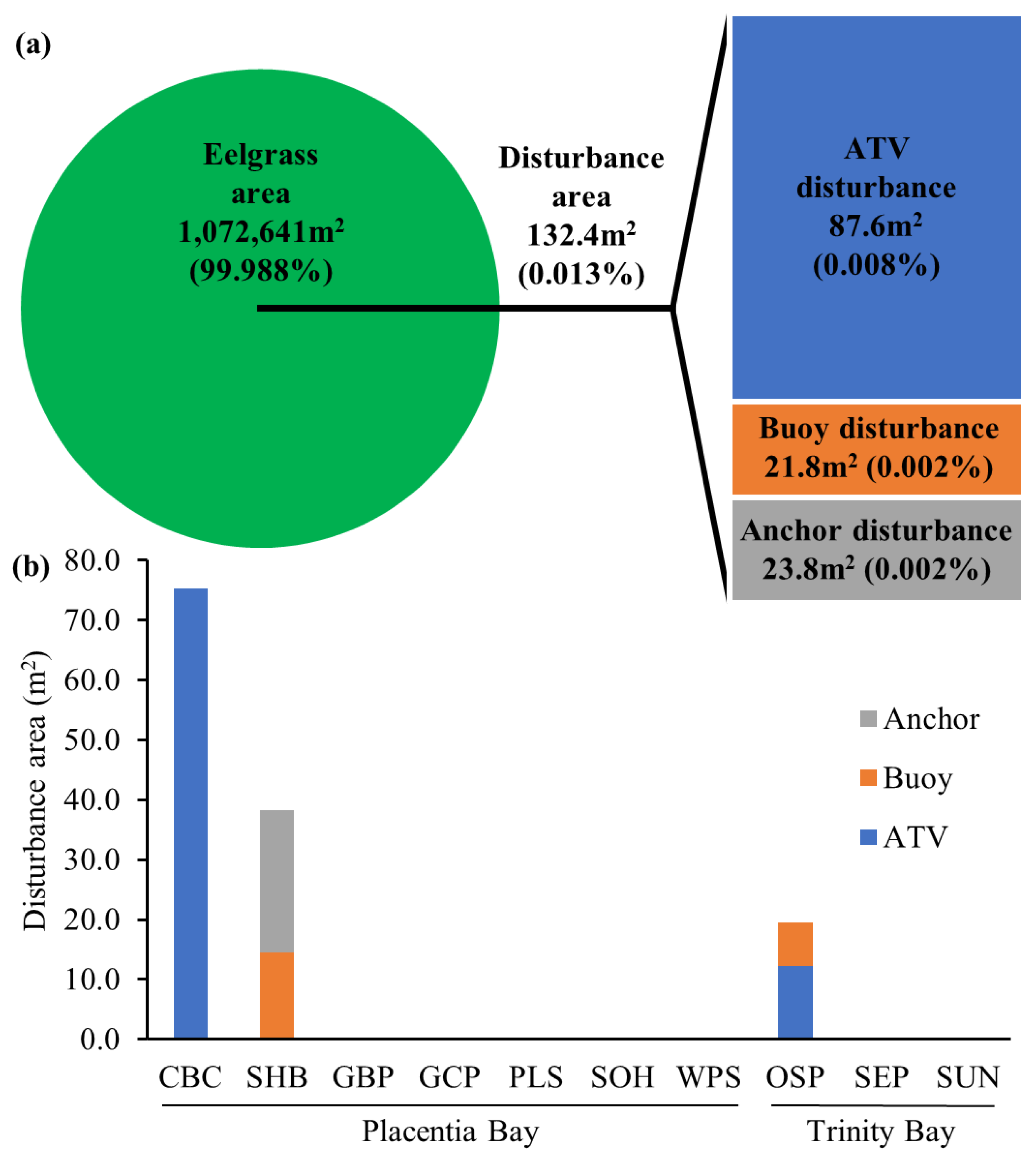
3.3. Anthropogenic Disturbances

Five occurrences of anthropogenic physical disturbances were identified from the aerial imagery, caused by three activities: all-terrain vehicles (ATVs) driving in eelgrass areas, buoys, and boat anchoring (Figure 4). Physical disturbances affected an approximate area of 132.4 m2, corresponding to only 0.013% of the total area of eelgrass mapped (Table 2 and Figure 5).
Indications of ATV use were observed at all sites, but disturbances rarely occurred in areas of eelgrass. ATV tracks were common throughout the sites, particularly concentrated on beaches and deltas, away from eelgrass. ATV tracks caused disturbance to eelgrass at Come by Chance Gut and Old Shop Pond. ATV tracks were observed in approximately 87.6 m2 of eelgrass, corresponding to a disturbance area of 0.008% of total eelgrass area.
Twelve buoys were observed in eelgrass areas, with five of them marking fishing gear while seven others were associated with docking infrastructure. Two buoys associated with docking infrastructure at Old Shop Pond and Ship Harbour created disturbances due to ropes dragging in the sediment with a combined area of ~21 m2. The other buoys did not create visible disturbances.
Anchoring within the eelgrass meadow was observed in the field at Ship Harbour. Eelgrass in the surrounding area varied in density with some barren patches. The anchoring disturbance, however, did not create a disturbance characteristic of anchoring damage. The disturbance area associated with anchoring was estimated to be 23.8 m2.

3.4. Semi-Quantitative Epiphyte Cover

Placentia Swans was the only site to have a large presence of epiphytes. When eelgrass was present in the video, approximately 27% of the video had no epiphyte cover, 49% had between 120% epiphyte cover, and 24% had over 20% epiphyte cover (half of it with 60–80% epiphyte cover) (Figure 6). At all other sites, the presence of epiphytes was minimal. However, at western Placentia Southeast Arm, tannin-rich freshwater inputs from heavy rainfall in the days preceding the video collection reduced the video quality, and potentially reduced epiphyte detectability. At western Placentia Southeast Arm, a dense algal cover was observed during field visits (Figure 6c).

4. Discussion

Our study mapped the distribution of eelgrass at seven sites of Placentia Bay and three sites of Trinity Bay, offering geographic baseline datasets for eelgrass on the island of Newfoundland. Very few anthropogenic physical disturbances were detected across the sites, and only one site, Placentia Swans, had a proliferation of epiphytes that could indicate nutrient enrichment (Table 2). These results suggest a minimal impact of physical disturbance and eutrophication on eelgrass in Placentia Bay and Trinity Bay; however, a larger number of study sites would be required to confirm the minimal impact of physical disturbance and eutrophication throughout the entirety of both bays.

4.1. Presence of Anthropogenic Stressors

Recreational vehicle disturbance has been shown to cause a decrease in saltmarsh vegetation cover [59]. The impact is most evident in areas with high track density, but reductions to vegetation cover can also occur in areas with a single track [59]. Come By Chance and Old Shop Pond were the only sites to have ATV disturbance. Come By Chance was classified with lower human presence due to the absence of anthropogenic structures and distance from a community, but this does not mean that human activities are absent from the site. There were indications of ATV use at all sites but mostly on land or in the intertidal zones, and rarely in areas occupied by eelgrass. In contrast to other regions where seagrass grows in the intertidal zone and disturbance from recreational vehicles is more common [60], eelgrass in Newfoundland rarely grows in the intertidal zone or shallow subtidal [20], due to winter ice damage [26]. The water depth in areas of eelgrass may deter ATV users and may explain why there are few instances of eelgrass disturbance caused by ATVs despite indications of ATV use in other parts of the study sites. During field visits, the eastern half of the eelgrass meadow at Come By Chance was submerged by only a few centimeters of water, differing from the upper depth limit for Newfoundland eelgrass (~1 m depth) described by Murphy et al. [20]. The shallow nature of the eelgrass meadow at Come By Chance during low tide may make the depth of water over the eelgrass area traversable by ATV. Similarly, at Old Shop Pond, ATV disturbance was observed in small patches of shallow eelgrass along the edge of a river delta.
The impact of mooring buoys on seagrass is well documented [35,36,61]. The area disturbed by buoys in the study sites remains very low (0.002%), when compared to the total area of eelgrass mapped and to other estimates of mooring buoy disturbances found in the literature. The mooring areas in this study have fewer moorings than other examples from the literature. For instance, in contrast to the seven buoys associated with docking infrastructure in this study creating a disturbance area of 21 m2, Unsworth et al. [36] identified 366 scars caused by moorings across eight sites creating an estimated total disturbance area of 3.71 hectares, and Glasby and West [35] estimated that leased moorings (1914 moorings) across New South Wales, Australia, caused ~22.4 hectares of disturbance to seagrasses.
Only one instance of anchoring within an eelgrass meadow was observed. The disturbance associated with anchoring at Ship Harbour was not a clear disturbance pattern. The presence of a lower density of eelgrass and barren patches suggest that anchoring may periodically occur in the same area but could also be natural variation in eelgrass density. This highlights a limitation in identifying physical disturbances using aerial imagery and underwater video without consistent temporal monitoring. If anchoring was not observed in this area during field visits, we may not have been able to identify this barren patch as a potential disturbance. If disturbances are created without a clear pattern, typical of common sources of disturbance (e.g., propeller scarring or mooring chains), they will likely not be detected when the source is no longer present for identification. Therefore, the number of physical disturbances identified may be underestimated due to the limited ability to determine if barren patches are of anthropogenic origin or naturally occurring. For instance, in Ship Harbour, two semi-circle disturbances with a diameter of ~6 m and a disturbance width of ~1 m were observed in both the ortho imagery and with underwater video (Figure S12). The regular shape of these disturbances suggests an anthropogenic source, but we were unable to identify the source of these disturbances.
Epiphytes, an indication of nutrient enrichment, were mostly observed at one study site: Placentia Swans. This site is adjacent to the town of Placentia, the largest town along the eastern shore of Placentia Bay, with a population of ~3500 [62]. Previous reports have indicated that untreated sewage may accumulate in some of the sheltered embayments of Placentia Bay [28], which may be the case here as there are drainages from the town of Placentia that empty directly into this site (Figure S13). Other factors, such as hydrodynamics [63,64], may also affect the presence of epiphytes across the study sites. The western portion of Placentia Southeast Arm, also adjacent to the town of Placentia, with a sewage outlet draining directly into the site, had minimal observations of epiphytes in the underwater video. Poor video quality, due to heavy rainfall and a large tannin-rich freshwater input in the days preceding underwater video collection, may have reduced epiphyte detectability at western Placentia Southeast Arm. However, a dense algal cover was observed at the site during UAV image collection. While there were indications of nutrient enrichment at the two sites adjacent to the town of Placentia, both sites have dense eelgrass meadows. This suggests that the current level of eutrophication may not be affecting eelgrass meadows in the area, yet. Based on the observations made in the western Placentia Southeast Arm and in Placentia Swans, it is recommended that these two sites be subjected to a more comprehensive examination, including a detailed analysis of trends in seagrass bed degradation, an identification of key driving factors, and potential conservation strategies.
This study observed eelgrass meadows growing adjacent to anthropogenic development but, at the moment, there appears to be little presence of anthropogenic disturbance. The communities in the surrounding areas of sites in this study have small human populations, the largest being the town of Placentia with a population of ~3500 [62], resulting in a smaller disturbance area and less nutrient pollution relative to regions where these stressors are more prevalent, such as the USA [65], Europe [15], and Australia [61]. Physical disturbances and proliferations of epiphytes appear to occur infrequently in eelgrass meadows of Placentia Bay and Trinity Bay. However, we were only able to survey a handful of sites. Stressors to eelgrass can vary locally [66]. For instance, the impact of boating activities on submerged aquatic vegetation can be highly variable and site-specific characteristics may influence the effect [67]. As such, our findings cannot be easily generalized to other eelgrass meadows of Placentia Bay and Trinity Bay that could not be surveyed.

4.2. Image Segmentation

In OBIA, the image segmentation step is largely regarded as the most critical step for a well-performing classification. Lourenço et al. [68] found that the accuracy of thematic vegetation maps produced using ArcGIS’ mean shift segmentation was worse than that of eCognition, a common proprietary software used for OBIA, and Orfeo Toolbox/Monteverdi (OTB), an open source OBIA software. For instance, the difference between overall accuracy (OA) was small between ArcGIS and OTB, with values of 84.3% and 87.0%, respectively, with a larger difference when compared to eCognition (OA = 95.7%) [68]. Similarly, for multiclass thematic vegetation maps of UAV imagery, Gonçalves et al. [48] found that ArcGIS produced a Kappa index of 0.78 compared to 0.85 for RGISLib’s Shepherd segmentation algorithm, and a Kappa of 0.96, the highest Kappa value, for single-class thematic vegetation maps. Perhaps, image segmentation conducted with an alternative segmentation software would result in different thematic map accuracy assessments, but potential gains in map accuracy may be small. Previous studies have compared the performance of different segmentation software in terrestrial environments [48,68,69,70], but future studies could compare the performance of different segmentation software specifically for mapping optically shallow coastal habitats where the optical properties of water and water depth create more subtle and smooth transitions between image objects.

4.3. Monitoring Recommendations

Monitoring seagrass beds can help fill critical data gaps for informing sustainable coastal management. UAVs provide a cost-effective solution for acquiring high-resolution imagery to monitor seagrass beds. However, the use of UAVs for monitoring seagrass beds is dependent on research objectives. For meadow-scale surveys, UAVs provide users with greater flexibility to control the frequency and timing of observations when compared to alternative remote sensing methods. This flexibility is particularly beneficial in regions where cloud cover would regularly impact optical satellite observations. The high-resolution imagery of UAVs also enables the monitoring of disturbances to seagrass beds. Small area disturbances may go unnoticed if the size of the disturbance is less than the spatial resolution of the image sensor. For instance, the disturbances mapped in this study would not be distinguishable in 10 m spatial resolution Sentinel-2 optical imagery. Additionally, the scale of the research objectives is important to consider and presents a limitation of UAV seagrass monitoring. For regional assessments, the use of satellite imagery would be imperative to survey an entire region. For instance, Traganos et al. [71] mapped 2510.1 km2 of Posidonia oceanica in the Aegean and Ionian Seas using Sentinel-2 imagery. Mapping such an extent with UAVs would be unfeasible.
The reproducibility of UAV surveys may also prove challenging due to the impacts of environmental conditions (e.g., surface rippling and cloud cover) on image classification for UAV imagery [27]. Prystay et al. [27] conducted seasonal UAV monitoring of seagrass beds and found inconsistent misclassification between their seasonal image classifications, which resulted in the inability to detect micro-/meso-scale changes. Prystay et al. [27] recommends the use of UAV surveys in concert with ground surveys. UAVs benefit monitoring programs by quantifying seagrass meadows at a macro-scale (e.g., seagrass extent) and ground surveys (e.g., snorkel surveys, quadrats, and monitoring stations) provide micro-scale details such as seagrass shoot density and fragmentation [27]. Integrating a variety of scales of monitoring was shown to be an effective method for detecting changes in seagrass ecosystems [72]. Ultimately, the objectives of a monitoring program and the quantitative metrics for determining objective progress will determine the scale and method of data collection.

5. Conclusions

This study looked at the spatial distribution of eelgrass in Placentia Bay, an area of Canada’s east coast where eelgrass has declined due to the invasive European green crab [22], and Trinity Bay, an adjacent area where this species is currently absent. Detailed data on eelgrass are rarely available, impacting our ability to monitor and understand changes in this important ecosystem often degraded in coastal environments. Findings indicate variable eelgrass extent in embayments of Placentia Bay and Trinity Bay. The study offers a baseline for monitoring future distributional changes in eelgrass that could be caused by European green crab or other environmental changes. The restoration of lost eelgrass due to the European green crab may be challenging until invasive European green crab populations are effectively managed or decline [73]. Future studies will be required to assess the effectiveness of eelgrass restoration in areas invaded by the European green crab. Baseline data from this study contribute to addressing a lack of data regarding the extent of Canadian seagrass. The results also suggest that, currently, there is little anthropogenic impact from physical disturbance and eutrophication on eelgrass in Placentia Bay and Trinity Bay. The limited number of disturbances and generally low epiphyte cover observed are likely due to the low populations of the communities in proximity to the eelgrass meadows. Changes to anthropogenic activities or environmental changes may impact eelgrass in the region. The continued monitoring of eelgrass and of its stressors in Placentia Bay is critical to continue to inform conservation and management efforts for this critical coastal ecosystem and to ensure the sustainability of coastal social–ecological systems that benefit from those species.

Supplementary Materials

The following supporting information can be downloaded at: https://www.mdpi.com/article/10.3390/su16083471/s1, Supplementary methods: SegOptim Parameter Space Delineation, Figure S1: Underwater image examples of epiphyte cover classes observed at the Placentia Swans site. Figure S2: Come By Chance Gut orthomosaic and thematic map, Table S1: Come By Chance Gut confusion matrix, Figure S3: Glennons Cove Pond orthomosaic and thematic map, Table S2: Glennons Cove Pond confusion matrix, Figure S4: Great Barasway Pond orthomosaic and thematic map, Table S3: Great Barasway Pond confusion matrix, Figure S5: Old Shop Pond orthomosaic and thematic map, Table S4: Old Shop Pond confusion matrix, Figure S6: Placentia Swans orthomosaic and thematic map, Table S5: Placentia Swans confusion matrix, Figure S7: Ship Harbour orthomosaic and thematic map, Table S6: Ship Harbour confusion matrix, Figure S8: Southern Harbour orthomosaic and thematic map, Table S7: Southern Harbour confusion matrix, Figure S9: Spread Eagle Pond orthomosaic and thematic map, Table S8: Spread Eagle Pond confusion matrix, Figure S10: Frenchmans Island orthomosaic and thematic map, Table S9: Frenchmans Island confusion matrix, Figure S11: Western Placentia Southeast Arm orthomosaic and thematic map, Table S10: Western Placentia Southeast Arm confusion matrix, Figure S12: Unknown eelgrass disturbance observed at Ship Harbour, Figure S13: Observed drainage locations from the town of Placentia.

Author Contributions

Conceptualization, A.S., R.D., K.R., A.L.B. and E.E.; Methodology, A.S., R.D., K.R., A.L.B. and E.E.; Formal Analysis, A.S.; Data Curation, A.S.; Writing—Original Draft Preparation, A.S.; Writing—Review and Editing, A.S., R.D., K.R., A.L.B. and E.E.; Supervision, R.D. and E.E.; Project Administration, K.R.; Funding Acquisition, R.D., K.R. and E.E. All authors have read and agreed to the published version of the manuscript.

Funding

This research was funded by the Fisheries and Oceans Canada’s Coastal Environmental Baseline Program as part of the ‘Coastal habitat mapping of Placentia Bay’ project. AS was also supported through Memorial University School of Graduate Studies’ baseline funding.

Institutional Review Board Statement

Not applicable.

Informed Consent Statement

Not applicable.

Data Availability Statement

Eelgrass distribution maps from this research are available through the National Eelgrass Dataset For Canada (NETForce) (https://open.canada.ca/data/en/dataset/a733fb88-ddaf-47f8-95bb-e107630e8e62, accessed on 17 April 2024).

Acknowledgments

The authors would like to acknowledge the assistance of Poppy Keogh, Kate Charmley, Rylan Command, Brandon Tilley, and Shreya Nemani (Memorial University) during fieldwork and Christophe Revillion (Université de la Réunion) for his guidance with object-based image analysis.

Conflicts of Interest

The authors declare no conflicts of interest.

References

  1. Green, E.P.; Short, F.T. World Atlas of Seagrasses; University of California Press: Berkeley, CA, USA, 2004; Volume 41, ISBN 0520240472. [Google Scholar]
  2. Costanza, R.; D’Arge, R. The Value of the World’s Ecosystem Services and Natural Capital. Nature 1997, 387, 253–260. [Google Scholar] [CrossRef]
  3. Nordlund, L.M.; Unsworth, R.K.F.; Gullström, M.; Cullen-Unsworth, L.C. Global Significance of Seagrass Fishery Activity. Fish Fish. 2018, 19, 399–412. [Google Scholar] [CrossRef]
  4. Unsworth, R.K.F.; Nordlund, L.M.; Cullen-Unsworth, L.C. Seagrass Meadows Support Global Fisheries Production. Conserv. Lett. 2019, 12, e12566. [Google Scholar] [CrossRef]
  5. Paul, M. The Protection of Sandy Shores—Can We Afford to Ignore the Contribution of Seagrass? Mar. Pollut. Bull. 2018, 134, 152–159. [Google Scholar] [CrossRef] [PubMed]
  6. Duarte, C.M.; Losada, I.J.; Hendriks, I.E.; Mazarrasa, I.; Marbà, N. The Role of Coastal Plant Communities for Climate Change Mitigation and Adaptation. Nat. Clim. Chang. 2013, 3, 961–968. [Google Scholar] [CrossRef]
  7. Fourqurean, J.W.; Duarte, C.M.; Kennedy, H.; Marbà, N.; Holmer, M.; Mateo, M.A.; Apostolaki, E.T.; Kendrick, G.A.; Krause-Jensen, D.; McGlathery, K.J.; et al. Seagrass Ecosystems as a Globally Significant Carbon Stock. Nat. Geosci. 2012, 5, 505–509. [Google Scholar] [CrossRef]
  8. Nordlund, L.M.; Koch, E.W.; Barbier, E.B.; Creed, J.C. Seagrass Ecosystem Services and Their Variability across Genera and Geographical Regions. PLoS ONE 2016, 11, e0163091. [Google Scholar] [CrossRef] [PubMed]
  9. Borum, J.; Duarte, C.; Krause-Jensen, D.; Greve, T.M. European Seagrasses: An Introduction to Monitoring and Management; The M&M Project: Copenhagen, Denmark, 2004; ISBN 8789143213. [Google Scholar]
  10. Güreşen, A.; Güreşen, S.O.; Aktan, Y. Combined Synthetic and Biotic Indices of Posidonia Oceanica to Qualify the Status of Coastal Ecosystems in the North Aegean. Ecol. Indic. 2020, 113, 106149. [Google Scholar] [CrossRef]
  11. Kerninon, F.; Payri, C.E.; Le Loc’h, F.; Alcoverro, T.; Maréchal, J.P.; Chalifour, J.; Gréaux, S.; Mège, S.; Athanase, J.; Cordonnier, S.; et al. Selection of Parameters for Seagrass Management: Towards the Development of Integrated Indicators for French Antilles. Mar. Pollut. Bull. 2021, 170, 112646. [Google Scholar] [CrossRef] [PubMed]
  12. Martínez-Crego, B.; Vergés, A.; Alcoverro, T.; Romero, J. Selection of Multiple Seagrass Indicators for Environmental Biomonitoring. Mar. Ecol. Prog. Ser. 2008, 361, 93–109. [Google Scholar] [CrossRef]
  13. Orth, R.J.; Carruthers, T.J.B.; Dennison, W.C.; Duarte, C.M.; Fourqurean, J.W.; Heck, K.L.; Hughes, A.R.; Kendrick, G.A.; Kenworthy, W.J.; Olyarnick, S.; et al. A Global Crisis for Seagrass Ecosystems. Bioscience 2006, 56, 987–996. [Google Scholar] [CrossRef]
  14. Waycott, M.; Duarte, C.M.; Carruthers, T.J.B.; Orth, R.J.; Dennison, W.C.; Olyarnik, S.; Calladine, A.; Fourqurean, J.W.; Heck, K.L.; Hughes, A.R.; et al. Accelerating Loss of Seagrasses across the Globe Threatens Coastal Ecosystems. Proc. Natl. Acad. Sci. USA 2009, 106, 12377–12381. [Google Scholar] [CrossRef] [PubMed]
  15. de los Santos, C.B.; Krause-Jensen, D.; Alcoverro, T.; Marbà, N.; Duarte, C.M.; van Katwijk, M.M.; Pérez, M.; Romero, J.; Sánchez-Lizaso, J.L.; Roca, G.; et al. Recent Trend Reversal for Declining European Seagrass Meadows. Nat. Commun. 2019, 10, 3356. [Google Scholar] [CrossRef] [PubMed]
  16. Lefcheck, J.S.; Orth, R.J.; Dennison, W.C.; Wilcox, D.J.; Murphy, R.R.; Keisman, J.; Gurbisz, C.; Hannam, M.; Brooke Landry, J.; Moore, K.A.; et al. Long-Term Nutrient Reductions Lead to the Unprecedented Recovery of a Temperate Coastal Region. Proc. Natl. Acad. Sci. USA 2018, 115, 3658–3662. [Google Scholar] [CrossRef] [PubMed]
  17. Krause-Jensen, D.; Duarte, C.M.; Sand-Jensen, K.; Carstensen, J. Century-Long Records Reveal Shifting Challenges to Seagrass Recovery. Glob. Chang. Biol. 2020, 27, 563–575. [Google Scholar] [CrossRef] [PubMed]
  18. McKenzie, L.J.; Nordlund, L.M.; Jones, B.L.; Cullen-Unsworth, L.C.; Roelfsema, C.; Unsworth, R.K.F. The Global Distribution of Seagrass Meadows. Environ. Res. Lett. 2020, 15, 074041. [Google Scholar] [CrossRef]
  19. Unsworth, R.K.F.; McKenzie, L.J.; Collier, C.J.; Cullen-Unsworth, L.C.; Duarte, C.M.; Eklöf, J.S.; Jarvis, J.C.; Jones, B.L.; Nordlund, L.M. Global Challenges for Seagrass Conservation. Ambio 2019, 48, 801–815. [Google Scholar] [CrossRef] [PubMed]
  20. Murphy, G.E.P.; Dunic, J.C.; Adamczyk, E.M.; Bittick, S.J.; Côté, I.M.; Cristiani, J.; Geissinger, E.A.; Gregory, R.S.; Lotze, H.K.; O’Connor, M.I.; et al. From Coast to Coast to Coast: Ecology and Management of Seagrass Ecosystems across Canada. Facets 2021, 6, 139–179. [Google Scholar] [CrossRef]
  21. DFO. Does Eelgrass (Zostera marina) Meet the Criteria as an Ecologically Significant Species? CSAS Sci. Advis. Rep. 2009, 18, 11. [Google Scholar]
  22. Matheson, K.; McKenzie, C.H.; Gregory, R.S.; Robichaud, D.A.; Bradbury, I.R.; Snelgrove, P.V.R.; Rose, G.A. Linking Eelgrass Decline and Impacts on Associated Fish Communities to European Green Crab Carcinus Maenas Invasion. Mar. Ecol. Prog. Ser. 2016, 548, 31–45. [Google Scholar] [CrossRef]
  23. Blakeslee, A.M.H.; McKenzie, C.H.; Darling, J.A.; Byers, J.E.; Pringle, J.M.; Roman, J. A Hitchhiker’s Guide to the Maritimes: Anthropogenic Transport Facilitates Long-Distance Dispersal of an Invasive Marine Crab to Newfoundland. Divers. Distrib. 2010, 16, 879–891. [Google Scholar] [CrossRef]
  24. Davis, R.C.; Short, F.T.; Burdick, D.M. Quantifying the Effects of Green Crab Damage to Eelgrass Transplants. Restor. Ecol. 1998, 6, 297–302. [Google Scholar] [CrossRef]
  25. Warren, M.A.; Gregory, R.S.; Laurel, B.J.; Snelgrove, P.V.R. Increasing Density of Juvenile Atlantic (Gadus morhua) and Greenland Cod (G. ogac) in Association with Spatial Expansion and Recovery of Eelgrass (Zostera marina) in a Coastal Nursery Habitat. J. Exp. Mar. Biol. Ecol. 2010, 394, 154–160. [Google Scholar] [CrossRef]
  26. Rao, A.S.; Gregory, R.S.; Murray, G.; Ings, D.W.; Coughlan, E.J.; Newton, B.H. Eelgrass (Zostera marina) Locations in Newfoundland and Labrador; Fisheries and Oceans Canada: St. John’s, NL, Canada, 2014. [Google Scholar]
  27. Prystay, T.S.; Adams, G.; Favaro, B.; Gregory, R.S.; Le Bris, A. The Reproducibility of Remotely Piloted Aircraft Systems to Monitor Seasonal Variation in Submerged Seagrass and Estuarine Habitats. Facets 2023, 8, 1–22. [Google Scholar] [CrossRef]
  28. DFA. Issues Scan of Selected Coastal and Ocean Areas of Newfoundland and Labrador. 2007. Available online: https://www.gov.nl.ca/ffa/files/publications-archives-pdf-issues-scan-of-selected-coastal-areas-of-newfoundland-and-labrador.pdf (accessed on 17 April 2024).
  29. LGL. Placentia Bay Atlantic Salmon Aquaculture Project Environmental Protection Plan (EPP): RAS Hatchery Operations. 2020. Available online: https://www.gov.nl.ca/ecc/files/FA0159-GriegNL-EPP-RAS-Hatchery-Operations-2-Oct.-2020.pdf (accessed on 17 April 2024).
  30. Catto, N.R.; Hooper, R.G.; Anderson, M.R.; Scruton, D.A.; Meade, J.D.; Ollerhead, L.M.N.; Williams, U.P. Biological and Geomorphological Classification of Placentia Bay: A Preliminary Assessment; Canadian Technical Report of Fisheries and Aquatic Sciences 1488-5379 No. 2289; Fisheries and Oceans Canada: St. John’s, NL, Canada, 1999. [Google Scholar]
  31. Cullain, N.; McIver, R.; Schmidt, A.L.; Milewski, I.; Lotze, H.K. Potential Impacts of Finfish Aquaculture on Eelgrass (Zostera marina) Beds and Possible Monitoring Metrics for Management: A Case Study in Atlantic Canada. PeerJ 2018, 6, e5630. [Google Scholar] [CrossRef] [PubMed]
  32. Jones, B.L.; Cullen-Unsworth, L.C.; Unsworth, R.K.F. Tracking Nitrogen Source Using Δ15 N Reveals Human and Agricultural Drivers of Seagrass Degradation across the British Isles. Front. Plant Sci. 2018, 9, 329228. [Google Scholar] [CrossRef]
  33. Hallac, D.E.; Sadle, J.; Pearlstine, L.; Herling, F.; Shinde, D. Boating Impacts to Seagrass in Florida Bay, Everglades National Park, Florida, USA: Links with Physical and Visitor-Use Factors and Implications for Management. Mar. Freshw. Res. 2012, 63, 1117–1128. [Google Scholar] [CrossRef]
  34. Orth, R.J.; Lefcheck, J.S.; Wilcox, D.J. Boat Propeller Scarring of Seagrass Beds in Lower Chesapeake Bay, USA: Patterns, Causes, Recovery, and Management. Estuaries Coasts 2017, 40, 1666–1676. [Google Scholar] [CrossRef]
  35. Glasby, T.M.; West, G. Dragging the Chain: Quantifying Continued Losses of Seagrasses from Boat Moorings. Aquat. Conserv. Mar. Freshw. Ecosyst. 2018, 28, 383–394. [Google Scholar] [CrossRef]
  36. Unsworth, R.K.F.; Williams, B.; Jones, B.L.; Cullen-Unsworth, L.C. Rocking the Boat: Damage to Eelgrass by Swinging Boat Moorings. Front. Plant Sci. 2017, 8, 262774. [Google Scholar] [CrossRef] [PubMed]
  37. Eriander, L.; Laas, K.; Bergström, P.; Gipperth, L.; Moksnes, P.O. The Effects of Small-Scale Coastal Development on the Eelgrass (Zostera marina L.) Distribution along the Swedish West Coast—Ecological Impact and Legal Challenges. Ocean Coast. Manag. 2017, 148, 182–194. [Google Scholar] [CrossRef]
  38. Gladstone, W.; Courtenay, G. Impacts of Docks on Seagrass and Effects of Management Practices to Ameliorate These Impacts. Estuar. Coast. Shelf Sci. 2014, 136, 53–60. [Google Scholar] [CrossRef]
  39. Kelly, J.J.; Orr, D.; Takekawa, J.Y. Quantification of Damage to Eelgrass (Zostera marina) Beds and Evidence-Based Management Strategies for Boats Anchoring in San Francisco Bay. Environ. Manag. 2019, 64, 20–26. [Google Scholar] [CrossRef] [PubMed]
  40. La Manna, G.; Donno, Y.; Sarà, G.; Ceccherelli, G. The Detrimental Consequences for Seagrass of Ineffective Marine Park Management Related to Boat Anchoring. Mar. Pollut. Bull. 2015, 90, 160–166. [Google Scholar] [CrossRef] [PubMed]
  41. Wong, M.C.; Bravo, M.A.; Dowd, M. Ecological Dynamics of Zostera marina (Eelgrass) in Three Adjacent Bays in Atlantic Canada. Bot. Mar. 2013, 56, 413–424. [Google Scholar] [CrossRef]
  42. Nahirnick, N.K.; Reshitnyk, L.; Campbell, M.; Hessing-Lewis, M.; Costa, M.; Yakimishyn, J.; Lee, L. Mapping with Confidence; Delineating Seagrass Habitats Using Unoccupied Aerial Systems (UAS). Remote Sens. Ecol. Conserv. 2019, 5, 121–135. [Google Scholar] [CrossRef]
  43. Agisoft LLC Agisoft Metashape 2019. Agisoft LLC, St. Petersburg, Russia. Available online: https://www.agisoft.com/ (accessed on 17 April 2024).
  44. ESRI ArcGIS 2019. Environmental Systems Research Institute, Redlands, California, USA. Available online: https://www.esri.com/en-us/home (accessed on 17 April 2024).
  45. Nahirnick, N.K.; Hunter, P.; Costa, M.; Schroeder, S.; Sharma, T. Benefits and Challenges of UAS Imagery for Eelgrass (Zostera marina) Mapping in Small Estuaries of the Canadian West Coast. J. Coast. Res. 2019, 35, 673–683. [Google Scholar] [CrossRef]
  46. Blaschke, T. Object Based Image Analysis for Remote Sensing. ISPRS J. Photogramm. Remote Sens. 2010, 65, 2–16. [Google Scholar] [CrossRef]
  47. R Core Team. R: A Language and Environment for Statistical Computing 2020. R Foundation for Statistical Computing, Vienna, Austria. Available online: https://www.R-project.org/ (accessed on 17 April 2024).
  48. Gonçalves, J.; Pôças, I.; Marcos, B.; Mücher, C.A.; Honrado, J.P. SegOptim—A New R Package for Optimizing Object-Based Image Analyses of High-Spatial Resolution Remotely-Sensed Data. Int. J. Appl. Earth Obs. Geoinf. 2019, 76, 218–230. [Google Scholar] [CrossRef]
  49. Comaniciu, D.; Meer, P. Mean Shift: A Robust Approach toward Feature Space Analysis. IEEE Trans. Pattern Anal. Mach. Intell. 2002, 24, 603–619. [Google Scholar] [CrossRef]
  50. Chabot, D.; Dillon, C.; Shemrock, A.; Weissflog, N.; Sager, E.P.S. An Object-Based Image Analysis Workflow for Monitoring Shallow-Water Aquatic Vegetation in Multispectral Drone Imagery. ISPRS Int. J. Geo-Inform. 2018, 7, 294. [Google Scholar] [CrossRef]
  51. Ellis, S.L.; Taylor, M.L.; Schiele, M.; Letessier, T.B. Influence of Altitude on Tropical Marine Habitat Classification Using Imagery from Fixed-Wing, Water-Landing UAVs. Remote Sens. Ecol. Conserv. 2020, 2, 50–63. [Google Scholar] [CrossRef]
  52. Oldeland, J.; Revermann, R.; Luther-Mosebach, J.; Buttschardt, T.; Lehmann, J.R.K. New Tools for Old Problems—Comparing Drone- and Field-Based Assessments of a Problematic Plant Species. Environ. Monit. Assess. 2021, 193, 90. [Google Scholar] [CrossRef] [PubMed]
  53. Belgiu, M.; Drăgu, L. Random Forest in Remote Sensing: A Review of Applications and Future Directions. ISPRS J. Photogramm. Remote Sens. 2016, 114, 24–31. [Google Scholar] [CrossRef]
  54. Millard, K.; Richardson, M. On the Importance of Training Data Sample Selection in Random Forest Image Classification: A Case Study in Peatland Ecosystem Mapping. Remote Sens. 2015, 7, 8489–8515. [Google Scholar] [CrossRef]
  55. Papakonstantinou, A.; Stamati, C.; Topouzelis, K. Comparison of True-Color and Multispectral Unmanned Aerial Systems Imagery for Marine Habitat Mapping Using Object-Based Image Analysis. Remote Sens. 2020, 12, 554. [Google Scholar] [CrossRef]
  56. Moran, P. Notes on Continuous Stochastic Phenomena. Biometrika 1950, 37, 17–23. [Google Scholar] [CrossRef] [PubMed]
  57. Sim, J.; Wright, C.C. The Kappa Statistic in Reliability Studies: Use, Interpretation, and Sample Size Requirements. Phys. Ther. 2005, 85, 257–268. [Google Scholar] [CrossRef] [PubMed]
  58. Nelson, W.G. Development of an Epiphyte Indicator of Nutrient Enrichment: A Critical Evaluation of Observational and Experimental Studies. Ecol. Indic. 2017, 79, 207–227. [Google Scholar] [CrossRef] [PubMed]
  59. Kelleway, J. Ecological Impacts of Recreational Vehicle Use on Saltmarshes of the Georges River, Sydney. Wetl. Aust. 2006, 22, 52. [Google Scholar] [CrossRef]
  60. Martin, S.R.; Onuf, C.P.; Dunton, K.H. Assessment of Propeller and Off-Road Vehicle Scarring in Seagrass Beds and Wind-Tidal Flats of the Southwestern Gulf of Mexico. Bot. Mar. 2008, 51, 79–91. [Google Scholar] [CrossRef]
  61. Evans, S.M.; Griffin, K.J.; Blick, R.A.J.; Poore, A.G.B.; Vergés, A. Seagrass on the Brink: Decline of Threatened Seagrass Posidonia Australis Continues Following Protection. PLoS ONE 2018, 13, e0190370. [Google Scholar] [CrossRef] [PubMed]
  62. Canada, S. Census Profile, 2016 Census Placentia, Town [Census Subdivision], Newfoundland and Labrador and Division No. 1, Census Division [Census Division], Newfoundland and Labrador. Available online: https://www12.statcan.gc.ca/census-recensement/2016/dp-pd/prof/details/page.cfm?Lang=E&Geo1=CSD&Code1=1001240&Geo2=CD&Code2=1001&SearchText=Placentia&SearchType=Begins&SearchPR=01&B1=All&TABID=1&type=0 (accessed on 17 April 2024).
  63. Lavery, P.S.; Reid, T.; Hyndes, G.A.; Van Elven, B.R. Effect of Leaf Movement on Epiphytic Algal Biomass of Seagrass Leaves. Mar. Ecol. Prog. Ser. 2007, 338, 97–106. [Google Scholar] [CrossRef]
  64. Strand, J.A.; Weisner, S.E.B. Wave Exposure Related Growth of Epiphyton: Implications for the Distribution of Submerged Macrophytes in Eutrophic Lakes. Hydrobiologia 1996, 325, 113–119. [Google Scholar] [CrossRef]
  65. Orth, R.J.; Williams, M.R.; Marion, S.R.; Wilcox, D.J.; Carruthers, T.J.B.; Moore, K.A.; Kemp, W.M.; Dennison, W.C.; Rybicki, N.; Bergstrom, P.; et al. Long-Term Trends in Submersed Aquatic Vegetation (SAV) in Chesapeake Bay, USA, Related to Water Quality. Estuaries Coasts 2010, 33, 1144–1163. [Google Scholar] [CrossRef]
  66. Murphy, G.E.P.; Wong, M.C.; Lotze, H.K. A Human Impact Metric for Coastal Ecosystems with Application to Seagrass Beds in Atlantic Canada. Facets 2019, 4, 210–237. [Google Scholar] [CrossRef]
  67. Sagerman, J.; Hansen, J.P.; Wikström, S.A. Effects of Boat Traffic and Mooring Infrastructure on Aquatic Vegetation: A Systematic Review and Meta-Analysis. Ambio 2020, 49, 517–530. [Google Scholar] [CrossRef] [PubMed]
  68. Lourenço, P.; Teodoro, A.C.; Gonçalves, J.A.; Honrado, J.P.; Cunha, M.; Sillero, N. Assessing the Performance of Different OBIA Software Approaches for Mapping Invasive Alien Plants along Roads with Remote Sensing Data. Int. J. Appl. Earth Obs. Geoinf. 2021, 95, 102263. [Google Scholar] [CrossRef]
  69. Kavzoglu, T.; Tonbul, H. An Experimental Comparison of Multi-Resolution Segmentation, SLIC and K-Means Clustering for Object-Based Classification of VHR Imagery. Int. J. Remote Sens. 2018, 39, 6020–6036. [Google Scholar] [CrossRef]
  70. Teodoro, A.C. Comparison of Performance of Object-Based Image Analysis Techniques Available in Open Source Software (Spring and Orfeo Toolbox/Monteverdi) Considering Very High Spatial Resolution Data. J. Appl. Remote Sens. 2016, 10, 016011. [Google Scholar] [CrossRef]
  71. Traganos, D.; Aggarwal, B.; Poursanidis, D.; Topouzelis, K.; Chrysoulakis, N.; Reinartz, P. Towards Global-Scale Seagrass Mapping and Monitoring Using Sentinel-2 on Google Earth Engine: The Case Study of the Aegean and Ionian Seas. Remote Sens. 2018, 10, 1227. [Google Scholar] [CrossRef]
  72. Neckles, H.A.; Kopp, B.S.; Peterson, B.J.; Pooler, P.S. Integrating Scales of Seagrass Monitoring to Meet Conservation Needs. Estuaries Coasts 2012, 35, 23–46. [Google Scholar] [CrossRef]
  73. Neckles, H.A. Loss of Eelgrass in Casco Bay, Maine, Linked to Green Crab Disturbance. Northeast. Nat. 2015, 22, 478–500. [Google Scholar] [CrossRef]
Figure 1. Study sites for eelgrass mapping in Placentia Bay and Trinity Bay, Newfoundland and Labrador, Canada. The red box of the inset identifies the general study region.
Sustainability 16 03471 g001
Figure 2. Method of ground-truth data collection. (a) Operation of telescopic pole (I) with affixed Sony FDR-X3000 ActionCam (II). (b) The camera was affixed to the telescopic pole using a custom-built camera mount (III). (c) Ground-truth video observation transects (red lines) for Great Barasway Pond (GBP). Example ground-truth images are provided for (d) sediment, (e) eelgrass, and (f) brown algae.
Sustainability 16 03471 g002
Figure 3. Orthomosaic aerial image (a) and classified map (b) of Come By Chance Gut. Maps of Great Barasway Pond (c), Placentia Swans (d), Western Placentia Southeast Arm (e), and Glennons Cove Pond (f).
Sustainability 16 03471 g003
Figure 4. (a) All-terrain vehicle (ATV) disturbance area, (b) buoy disturbance area, (c) underwater image of buoy rope disturbance, (d) anchor disturbance area, and (e) underwater image of anchor in eelgrass meadow.
Sustainability 16 03471 g004
Figure 5. (a) Portion of disturbance area relative to the total area of eelgrass mapped. (b) Disturbance area at each site caused by anthropogenic activities. No disturbances were observed at GBP, GCP, PLS, SEP, SOH, SUN, or WPS. CBC: Come By Chance Gut; GBP: Great Barasway Pond; GCP: Glennons Cove Pond; PLS: Placentia Swans; OSP: Old Shop Pond; SEP: Spread Eagle Pond; SHB: Ship Harbour; SOH: Southern Harbour; SUN: Sunny Side; WPS: Western Placentia Southeast Arm.
Sustainability 16 03471 g005
Figure 6. (a) Proportion of underwater video duration by epiphyte cover category, measured as the amount of eelgrass in the video frame covered by epiphytes, when eelgrass was present in the ground-truth video at Placentia Swans. (b) Underwater image of epiphytes corresponding to the 61–80% epiphyte cover category. (c) Example of dense algal cover observed during field visits to western Placentia Southeast Arm.
Sustainability 16 03471 g006
Table 1. Accuracy assessments of eelgrass distribution maps and the area of eelgrass per site.
Study SiteMean KappaOverall Accuracy (%)Eelgrass Producer’s Accuracy (%)Eelgrass User’s Accuracy (%)Eelgrass Area (km2)
Come By Chance Gut0.71 ± 0.0882.2 ± 4.989.9 ± 9.087.9 ± 7.30.1310
Glennons Cove Pond0.67 ± 0.0882.2 ± 3.560.0 ± 43.573.3 ± 43.50.0013
Great Barasway Pond0.81 ± 0.0489.3 ± 2.898.4 ± 2.395.1 ± 0.40.0597
Old Shop Pond0.73 ± 0.1082.0 ± 6.988.5 ± 6.589.2 ± 9.70.0687
Placentia Swans0.46 ± 0.0769.7 ± 4.156.0 ± 5.262.1 ± 8.30.0916
Ship Harbour0.72 ± 0.0882.2 ± 5.191.7 ± 7.377.2 ± 10.90.0587
Southern Harbour0.61 ± 0.1575.8 ± 9.923.3 ± 14.948.8 ± 36.60.0054
Spread Eagle Pond0.65 ± 0.1484.7 ± 6.395.4 ± 3.890.0 ± 3.70.1967
Sunny Side0.69 ± 0.1080.3 ± 6.389.8 ± 5.681.0 ± 5.20.1265
Western Placentia Southeast Arm0.22 ± 0.2386.3 ± 3.199.2 ± 1.187.5 ± 3.00.3331
Table 2. Summary of the presence of physical disturbance and signs of eutrophication found across the ten study sites in Placentia Bay and Trinity Bay.
SiteBayEelgrass Area (km2)Disturbance Area (m2)Source of DisturbanceSigns of Eutrophication
Come By ChancePlacentia Bay0.131075.4ATV/
Glennons Cove PondPlacentia Bay0.0013///
Great Barasway PondPlacentia Bay0.0597///
Old Shop PondTrinity Bay0.068719.6ATV, buoy/
Placentia SwansPlacentia Bay0.0916//proliferation of epiphytes
Ship HarbourPlacentia Bay0.058738.3buoy, anchor/
Southern HarbourPlacentia Bay0.0054///
Spread Eagle PondTrinity Bay0.1967///
Sunny SideTrinity Bay0.1265///
Western Placentia Southeast ArmPlacentia Bay0.3331//floating algal mats
Disclaimer/Publisher’s Note: The statements, opinions and data contained in all publications are solely those of the individual author(s) and contributor(s) and not of MDPI and/or the editor(s). MDPI and/or the editor(s) disclaim responsibility for any injury to people or property resulting from any ideas, methods, instructions or products referred to in the content.

