A Time Series Prediction Model for Wind Power Based on the Empirical Mode Decomposition–Convolutional Neural Network–Three-Dimensional Gated Neural Network

Abstract

In response to the global challenge of climate change and the shift away from fossil fuels, the accurate prediction of wind power generation is crucial for optimizing grid operations and managing energy storage. This study introduces a novel approach by integrating the proportional–integral–derivative (PID) control theory into wind power forecasting, employing a three-dimensional gated neural (TGN) unit designed to enhance error feedback mechanisms. The proposed empirical mode decomposition (EMD)–convolutional neural network (CNN)–three-dimensional gated neural network (TGNN) framework starts with the pre-processing of wind data using EMD, followed by feature extraction via a CNN, and time series forecasting using the TGN unit. This setup leverages proportional, integral, and differential control within its architecture to improve adaptability and response to dynamic wind patterns. The experimental results show significant improvements in forecasting accuracy; the EMD–CNN–TGNN model outperforms both traditional models like autoregressive integrated moving average (ARIMA) and support vector regression (SVR), and similar neural network approaches, such as EMD–CNN–GRU and EMD–CNN–LSTM, across several metrics including mean absolute error (MAE), mean squared error (MSE), root mean squared error (RMSE), and coefficient of determination ($R^2$). These advancements substantiate the model’s effectiveness in enhancing the precision of wind power predictions, offering substantial implications for future renewable energy management and storage solutions.

1. Introduction

In the global context of actively addressing climate change and gradually reducing the dependence on fossil fuels [1], wind energy has emerged as a core element of energy diversification due to its cleanliness and sustainability. Accurate wind power prediction is crucial for grid operators, as it aids in the efficient management of power supply and demand, reduces energy waste, and significantly enhances the economic benefits of wind energy [2]. However, wind power prediction faces many challenges due to uncertainties such as the operational status of wind turbines and climatic conditions, exhibiting high non-linearity in wind power time series data [3,4], posing challenges to accurate forecasting.

Since Rumelhart introduced back-propagation in 1986, the development of neural networks has gone through several stages. In 1990, the Elman network enabled RNNs to handle time series, although it struggled with long-term dependencies. In 1997, the ability of the LSTM of meteorological factors to achieve satisfactory results with hybrid models remained a significant challenge.This study, based on the development trends of recurrent neural network units and hybrid models, experimentally integrates PID theory into recurrent neural units, effectively improving the accuracy of wind power prediction [5,6,7]. In recent years, researchers have primarily focused on integrating traditional algorithms with other methodologies in time series forecasting models [8]. For instance, the LSTM technique has also made significant progress in the field of wind power forecasting. In 2021, Shahid et al. [9] introduced a GLSTM model that combines LSTM with the genetic algorithm (GA), using the GA to optimize parameters in the model, focusing on feature learning and global optimization of non-linear sequential data, particularly optimizing the window size and number of neurons in the LSTM layers, which improved the wind power prediction performance by an average of 6% to 30%. In 2022, Xiang et al. [10] combined the self-attention temporal convolutional network (SATCN) with LSTM to create the SATCN–LSTM model. Here, the SATCN captures local features in time series data through convolutional layers, while the self-attention mechanism addresses long-range dependencies, thereby enhancing the model’s capacity to understand dynamic changes in time series data and increasing the accuracy of wind power forecasts, reducing the root mean square error by 17.56%. In 2023, Houran et al. combined LSTM with swarm intelligence (SI) optimization algorithms to develop a framework for short-term offshore wind power output estimation, wherein SI effectively searches the global space for optimal solutions to optimize LSTM model parameters, demonstrating excellent predictive performance in experiments. Also in 2023, Cui et al. [11] employed an improved dynamic sliding door algorithm (ImDSDA), Fuzzy C-Means (FCM), and a similarity matching mechanism in conjunction with an LSTM model to predict wind power ramp events, wherein ImDSDA dynamically adjusts gating parameters, FCM addresses overlapping data categories, and the similarity matching mechanism enhances the predictive capabilities under specific conditions, showing a performance superior to the existing methods in three mountainous wind farms in central China. Meanwhile, the application of a gated recurrent unit (GRU) in time series forecasting models continues to rise, particularly in the realm of wind power forecasting. For instance, in 2021, Kisvari et al. [12] introduced a GRU neural network method that integrates data pre-processing, resampling, anomaly detection and handling, feature engineering, and hyper-parameter tuning. This method displayed a clear advantage over traditional LSTM models in terms of prediction accuracy, training speed, and noise sensitivity, with a training speed increase of 38%. That same year, Liu et al. [13] developed a KK–CNN–GRU model guided by K-shape and K-means clustering, further expanding GRU’s application scope. “KK” in the KK–CNN–GRU method stands for K-shape and K-means clustering, used to extract patterns, denoise, and optimize input data, enhancing the model’s accuracy in wind power prediction. In Experiment A, KK–CNN–GRU achieved an RMSE of 83.6–224 kW and a MAPE of 4.36–18.7%; in Experiment B, the RMSE was in the range of 228–368 kW and the MAPE was in the range of 18.3–34.4%, showing high predictive accuracy. In 2023, Xiao et al. [14] introduced feature weighted principal component analysis (WPCA) and particle swarm optimization (PSO) algorithms to optimize the hyper-parameters of the GRU model. This method demonstrated significant advantages in actual wind power forecasting compared to other machine learning models, with reductions in the MAE and RMSE of 5.3–16% and 10–16%, respectively, and an increase in $R^2$ of 2.1–3.1%. Although these methods incorporate other algorithms to create hybrid models that mitigate the non-linearity and complexity of wind power forecasting, due to the non-stationary nature of meteorological factors, achieving satisfactory wind power forecasting results using hybrid models remains a significant challenge. Thus, this study builds upon the trends in recurrent neural network (RNN) units and hybrid models, experimentally incorporating PID theory into RNN units, effectively enhancing the accuracy of wind power prediction.

To provide a comprehensive performance comparison framework, this research will also employ traditional machine learning algorithms such as the autoregressive integrated moving average (ARIMA) model and support vector regression (SVR) as baseline models [15]. The ARIMA model is widely used in electricity demand and price forecasting due to its ability to handle the non-stationarity of time series data [16]. Meanwhile, SVR, as a powerful regression tool, has been proven to deliver satisfactory results in forecasting tasks with highly non-linear characteristics. By comparing with these traditional models, the aim is to demonstrate the accuracy of the EMD–CNN–TGNN model in predicting wind power.

In order to fully exploit the predictive capabilities of neural units for wind power time series data and enhance the accuracy of wind power prediction models, this study has undertaken the following tasks: (1) By integrating PID control theory and neural network technology, a three-dimensional gated neural (TGN) unit was designed based on error propagation. (2) Combined with the three-dimensional gated neural unit, the empirical mode decomposition (EMD)–convolutional neural network (CNN)–three-dimensional gated neural network (TGNN) was proposed. (3) The network model was experimentally validated using actual data from three wind farms, demonstrating its robust predictive capability.

Section 1 of this study provides a detailed background and highlights the cutting-edge achievements in the related literature. Section 2 supplies real operational data from three wind farms, providing an empirical basis for the research. Section 3 first describes the proposed EMD–CNN–TGNN model in detail, including the empirical mode decomposition (EMD) technique, the method of feature extraction through a convolutional neural network (CNN), and the foundational theory and prediction process of the three-dimensional gated neural network (TGNN). Section 4 presents the performance of the proposed model and other comparative models in experiments, validating its predictive efficacy. Finally, Section 5 offers conclusions and discussions.

2. Data and Evaluation Method

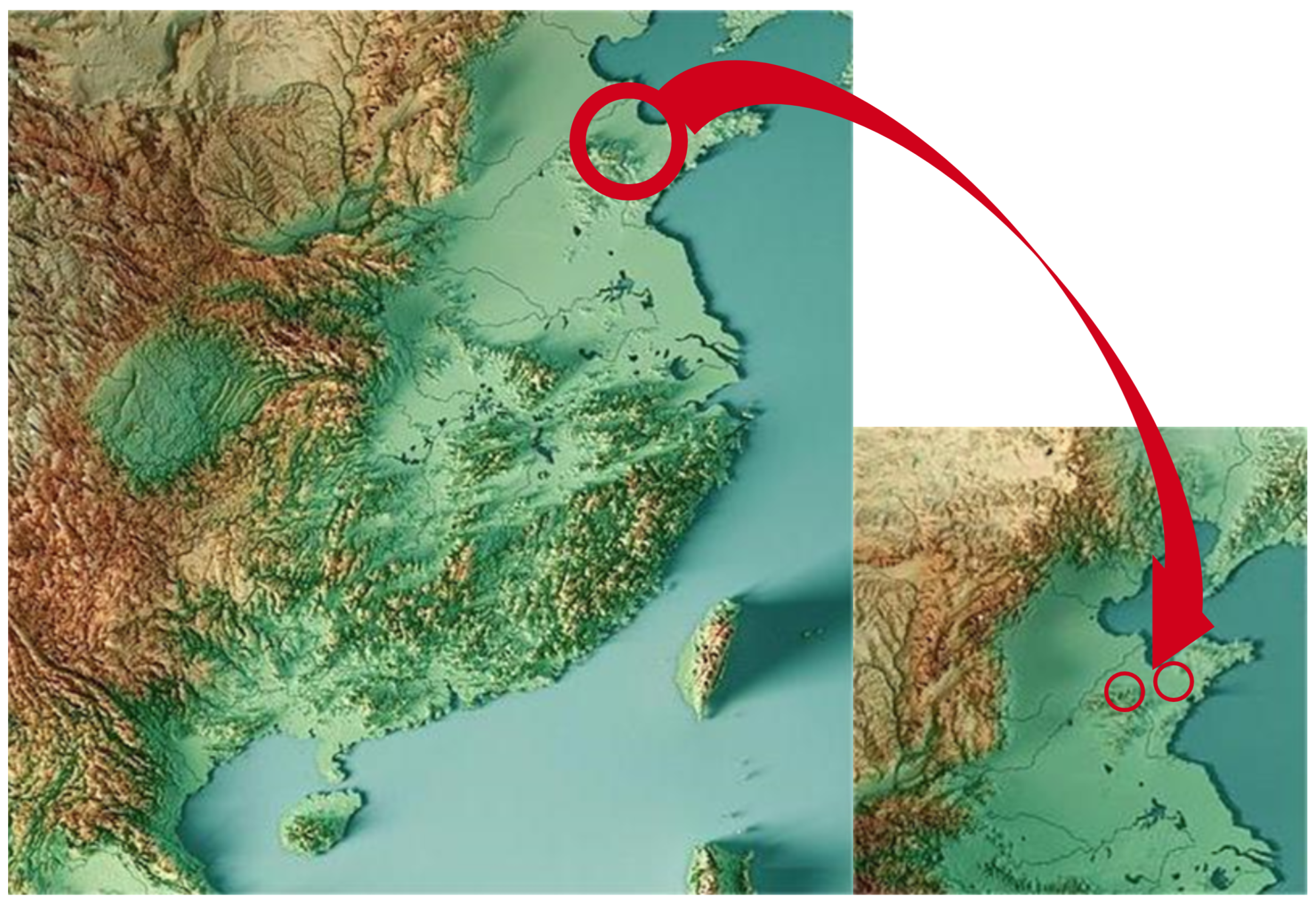
2.1. Wind Farm Data

To validate the predictive accuracy of our model, this study employed real data from two wind farms located in Xingtai, Hebei Province, and one in Dezhou, Shandong Province, China. The specific locations of these wind farms are illustrated in Figure 1, and the data include historical wind power generation data from each site with a temporal resolution of 10 min. All data underwent rigorous quality control procedures including the removal of erroneous data and the imputation of missing values. Detailed descriptions of these three wind farms are provided in

Table 1. Introduction to wind farm data.

Wind Farm	Terrain	Elevation (m)	Time Span
Wind Farm A	Plain	26–30.1	6 March 2021–5 March 2024
Wind Farm B	Plain	18.5	31 March 2021–29 February 2024
Wind Farm C	Plain	28–36	1 January 2022–31 December 2023

.

2.2. Data

Real data collected through SCADA systems provide a more accurate reflection of the operational conditions at wind farms. The SCADA system records data in 10-minute intervals, and the raw turbine data from the three wind farms are provided in “.csv” format [17]. Data from nine wind turbines across these farms are used to validate the model’s predictive accuracy.

Upon analyzing the wind data from the three wind farms (

Table 2. Wind farm A data.

Turbine	Max (kW)	Min (kW)	Median (kW)	Mean (kW)	Variance (kW)	Standard Deviation (kW)	Skewness (kW)	Kurtosis (kW)
A1	2336.60	0.00	382.28	702.70	584,459.00	764.50	0.97	0.44
A2	2335.97	0.00	405.64	734.90	622,922.48	789.25	0.90	0.61
A3	2336.70	0.00	411.91	740.92	626,814.16	791.72	0.89	0.63

The first uppercase letter represents the wind farm, and the second Arabic numeral indicates the wind turbine number. For example, “A1” refers to turbine number 1 of wind farm A.

,

Table 3. Wind farm B data.

Turbine	Max (kW)	Min (kW)	Median (kW)	Mean (kW)	Variance (kW)	Standard Deviation (kW)	Skewness (kW)	Kurtosis (kW)
B1	2200.10	0.00	321.90	634.51	513,606.25	716.66	0.99	0.44
B2	2200.10	0.00	289.00	609.82	507,952.22	712.71	1.06	0.30
B3	2200.10	0.00	277.60	594.64	495,569.65	703.97	1.10	0.20

The first uppercase letter represents the wind farm, and the second Arabic numeral indicates the wind turbine number. For example, “B1” refers to turbine number 1 of wind farm B.

and

Table 4. Wind farm C data.

Turbine	Max (kW)	Min (kW)	Median (kW)	Mean (kW)	Variance (kW)	Standard Deviation (kW)	Skewness (kW)	Kurtosis (kW)
C1	2248.59	0.00	419.49	752.98	676,617.35	822.57	0.76	0.96
C2	2249.91	0.00	387.54	728.84	677,555.42	823.14	0.83	0.84
C3	2244.22	0.00	341.04	687.23	640,244.73	800.15	0.91	0.66

The first uppercase letter represents the wind farm, and the second Arabic numeral indicates the wind turbine number. For example, “C1” refers to turbine number 1 of wind farm C.

), it was noted that the maximum outputs of all turbines are closely ranged between 2200 and 2336.7 kW, with a minimum output of 0 kW, indicating a definite lower output limit. Notably, turbine 1 of Wind Farm C exhibited higher wind power outputs in terms of average (752.98 kW) and median (419.49 kW) compared to turbine 3 of Wind Farm B, which had a lower average (594.64 kW) and median (277.6 kW). This variance highlights performance differences between turbines. All turbines exhibit significant volatility in wind power output, as indicated by the variance and standard deviation values, such as turbine 1 of Wind Farm C with a variance of 676,617.35 and a standard deviation of 822.57. The data distribution analysis shows a positive skewness across all turbines, indicating a rightward skew, while the negative kurtosis values suggest a relatively flat distribution.

These key data points allow us to conclude that, despite performance differences, all turbines show significant output fluctuations, which poses challenges for wind power prediction. For instance, the turbines in Wind Farm C generally perform better in terms of average and median wind power, but they also experience greater fluctuations, particularly turbine 1. Conversely, turbine 3 of Wind Farm B, while showing lower average wind power output, displays a more balanced data distribution, exhibiting the most significant data skew.

2.3. Evaluation Method

In the performance evaluation of regression models, four core metrics are employed: MAE (mean absolute error), MSE (mean squared error), RMSE (root mean squared error), and $R^2$ (coefficient of determination). These metrics evaluate the discrepancy between the model’s predictions and actual values, and the model’s explanatory power from various perspectives [8,18].

2.3.1. Core Metrics

• MAE (Mean Absolute Error) reflects the average deviation between predicted and actual values. It is robust against outliers and is defined as follows:

  $$\mathrm{MAE}=\frac{1}{n}\sum _{i=1}^n|y_i-{\widehat{y}}_i|$$

  (1)

  where $y_i$ is the actual value for the ith sample, ${\widehat{y}}_i$ is the model’s predicted value, and n is the total number of samples.
• MSE (Mean Squared Error) is the average of the squared differences between observed and predicted values, emphasizing larger errors:

  $$\mathrm{MSE}=\frac{1}{n}\sum _{i=1}^n{(y_i-{\widehat{y}}_i)}^2$$

  (2)
• RMSE (Root Mean Squared Error) provides a standard measure of error magnitude in the same units as the data:

  $$\mathrm{RMSE}=\sqrt{\frac{1}{n}\sum _{i=1}^n{(y_i-{\widehat{y}}_i)}^2}$$

  (3)
• $R^2$ (Coefficient of Determination) indicates the proportion of variance in the dependent variable predictable from the independent variables:

  $$R^2=1-\frac{{\sum }_{i=1}^n{(y_i-{\widehat{y}}_i)}^2}{{\sum }_{i=1}^n{(y_i-\overline{y})}^2}$$

  (4)

  where $\overline{y}$ is the mean of the actual values.

2.3.2. Performance Improvement Metric

To quantify performance differences between two models, the performance improvement (PI) metric is used:

$$\mathrm{PI}=\left(\frac{P_i-P_{i+1}}{P_{i+1}}\right)\times 100\%$$

(5)

where $P_i$ and $P_{i+1}$ are the performance metrics for the respective models.

3. Methods

3.1. Construction of EMD–CNN–TGNN

This research introduces a neural network architecture known as EMD–CNN–TGNN, which is based on error feedback. As depicted in Figure 2, the EMD-CNN–TGNN architecture initially utilizes empirical mode decomposition (EMD) to unfold the time series information. The resultant intrinsic mode functions (IMFs) are then compiled into a multi-resolution matrix, which is fed into a convolutional neural network (CNN) for feature extraction. Ultimately, the predictions are made using the three-dimensional gated neural network (TGNN).

3.1.1. EMD

Empirical mode decomposition (EMD) is an adaptive method used to analyze and process the non-linear and non-stationary characteristics of wind power. Each IMF component reflects the inherent oscillatory modes of wind power at different time scales, effectively identifying and predicting power fluctuation trends [19,20].

The core steps of EMD include:

• Extraction of Local Extrema: Identify all local extrema $p_1,p_2,\dots ,p_N$ in the given signal $x\left(t\right)$.
• Envelope Extraction: For each pair of adjacent local extrema $p_i$ and $p_{i+1}$, perform linear interpolation to derive the upper $e_{\max }\left(t\right)$ and lower $e_{\min }\left(t\right)$ envelopes:

  $$\begin{array}{cc}\hfill e_{\max }\left(t\right)& =\frac{p_{i+1}-p_i}{t_{i+1}-t_i}\times (t-t_i)+p_i\hfill \end{array}$$

  (6)

  $$\begin{array}{cc}\hfill e_{\min }\left(t\right)& =\frac{p_{i+1}-p_i}{t_{i+1}-t_i}\times (t-t_i)+p_i\hfill \end{array}$$

  (7)
• Extraction of IMFs: Subtract the mean envelope $e_{\mathrm{avg}}\left(t\right)$ from the signal $x\left(t\right)$ to obtain the first-order IMF $c_1\left(t\right)$. Repeat this process until $c_1\left(t\right)$ meets the stopping criteria to become the first IMF. Continue similarly until all IMFs are extracted.

Using the empirical mode decomposition method, 2048 wind power time series data points were decomposed into seven different IMFs. These IMFs were then assembled into a matrix of size $2048\times 7$, shown in Figure 3, to serve as input for the CNN.

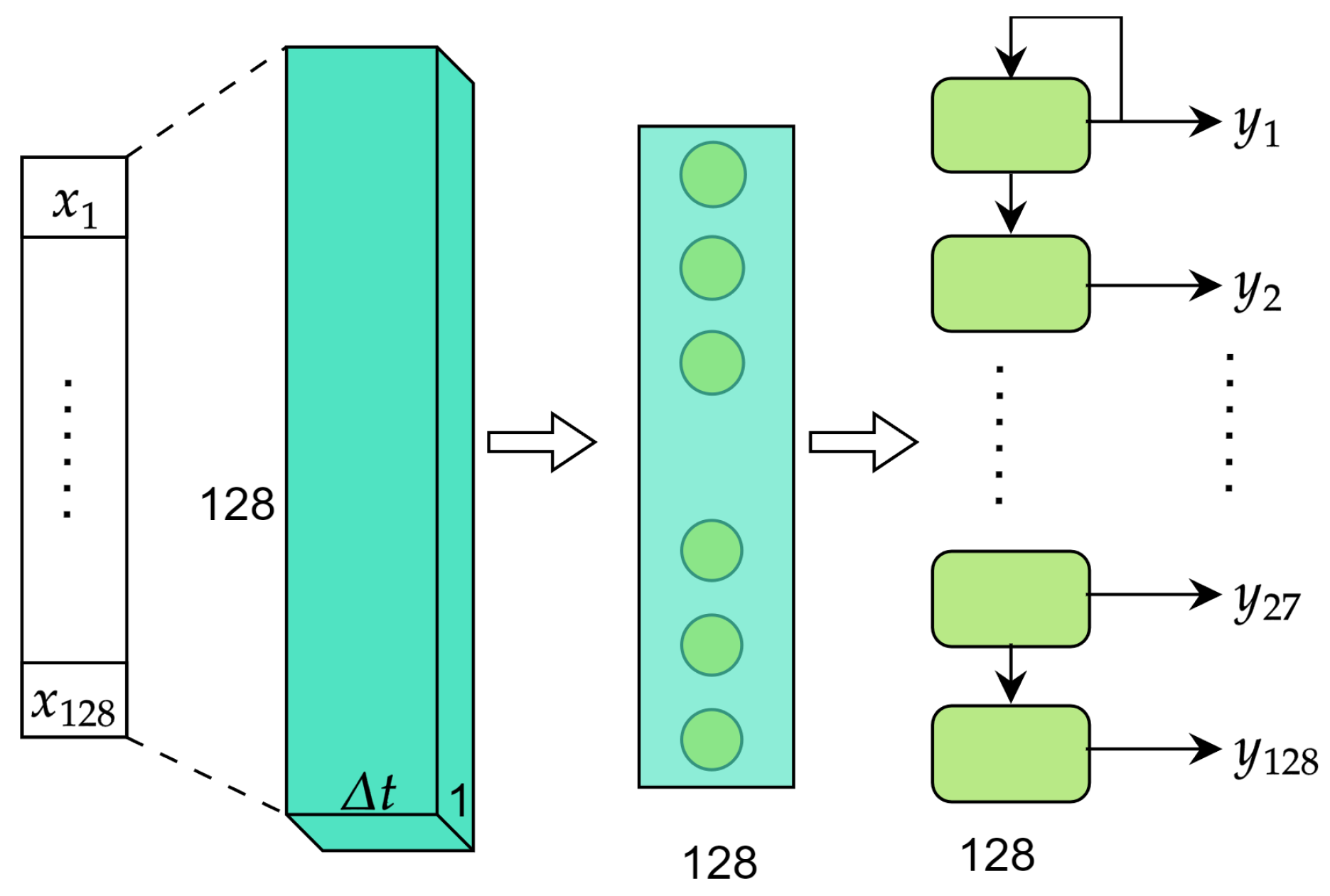
3.1.2. Construction of CNN

The convolutional neural network (CNN) is a robust deep learning model, instrumental in extracting hierarchical features from data through its layers of convolutions and pooling. In the realm of wind power data, the CNN adeptly learns characteristic patterns at various temporal resolutions, capturing both short-term and long-term trends. Wind power data, known for their complexity, often elude traditional feature extraction techniques, which the CNN circumvents by learning directly from raw data in an end-to-end manner. This method significantly simplifies the otherwise complex task of manual feature design.

The CNN architecture developed in this study comprises multiple convolutional layers, pooling layers, and a fully connected layer, as detailed in

Table 5. CNN model parameters.

Layer Type	Output Size	Kernel Size	Number of Filters	Activation Function	Remark
Input layer	2048 × 7 × 1	-	-	-	Input shape is 2048 × 7, 1 channel
Convolutional layer 1	2044 × 7 × 32	5 × 1	32	ReLU	Kernel stride is 1
Pooling layer 1	1022 × 7 × 32	2 × 1	-	-	Max pooling
Convolutional layer 2	1018 × 7 × 64	5 × 1	64	ReLU	Kernel stride is 1
Pooling layer 2	509 × 7 × 64	2 × 1	-	-	Max pooling
Flatten	227136 × 1	-	-	-	-
Fully connected layer	128 × 1	-	-	ReLU	-

. Designed to extract meaningful features from the intrinsic mode functions (IMFs) matrix, these features are then transformed into a vector of size $128\times 1$. This vector is utilized by subsequent layers of the three-dimensional gated neural (TGN) unit. Specifically, the initial layer of the model is a convolutional layer, which utilizes 32 filters of size $5\times 1$ to process the input matrix, employing the ReLU activation function to enhance the model’s capability to handle non-linearities. This is followed by a max pooling layer that uses a $2\times 1$ window to down-sample the feature map, thereby reducing computational demand while increasing the model’s abstraction capacity.

Subsequent convolutional and pooling layers deepen the learning process. The number of filters is increased to 64 to capture more complex features, maintaining the same kernel size and pooling strategy. This design not only bolsters the model’s feature extraction capabilities but also efficiently reduces the dimensionality of the features, laying a foundational framework for feature vector generation.

After two cycles of convolution and pooling, the feature map is flattened into a one-dimensional vector and processed through a fully connected layer. This layer, containing 128 neurons and utilizing the ReLU activation function, outputs a vector of size $128\times 1$. This vector, enriched with crucial information from the original time series data, represents a meticulously refined feature representation, providing robust support for the subsequent predictive tasks. The schematic of this layer structure is illustrated in Figure 4.

3.1.3. Construction of the Three-Dimensional Gated Neural (TGN) Unit

While LSTM and GRU units have been effective in managing complex and dynamic time series data, they have not fully addressed the nuances in temporal intervals between data points and the rate of increase in wind power output [21]. Considering the capabilities of PID control theory in handling time series data, a novel neural network unit based on error feedback has been proposed, where the initial error is set to zero. The network utilizes proportional and differential controls, employing the tanh function to manage the flow proportion of error to the model’s output at time t, denoted as $h_t$, and introduces an interval $\Delta t$ to calculate the rate of error change, thereby adjusting the impact at the current moment.

To address long-term dependencies, an integral gate mechanism is incorporated, which combines previous integration results with proportional control coefficients. The integration control coefficient at the current moment is calculated using the ReLU function, which helps in preventing gradient vanishing or explosion. Moreover, the error bias term $b_t$ in the model output $h_t$ is replaced by a three-dimensional gate, facilitating the transfer and predictive functionality of error information. The structure of the TGN is illustrated in Figure 5.

The mathematical representation of the TGN unit includes several key equations:

$$\begin{array}{}\mathrm{(8)}& e_0=0\hfill \mathrm{(9)}& e_t=y_t-{\widehat{y}}_t\hfill \mathrm{(10)}& p_t=tanh(w_{pt}·e_t+b_{pt})\hfill \mathrm{(11)}& i_t=\mathrm{ReLU}(w_{it}·p_t+i_{t-1}+b_{it})\hfill \mathrm{(12)}& d_t=tanh(w_{dt}·(e_t-e_{t-1})/\Delta t+b_{dt})\hfill \mathrm{(13)}& h_t=\sigma (w_h·h_{t-1}+w_x·x+b+p_t+i_t+d_t)\hfill \end{array}$$

Here, $e_0$ represents the initial error, assumed to be zero, indicating no error at the start. $e_t$ calculates the error at time step t, with $y_t$ being the actual observed value and ${\widehat{y}}_t$ the model’s predicted value. The prediction component $p_t$ utilizes the tanh activation function. The internal state $i_t$ at time t is computed using the ReLU function, with $i_{t-1}$ as the internal state from the previous time step. $d_t$ calculates the differential term with tanh as the activation function, and $\Delta t$ represents the time step length. Finally, $h_t$ represents the output of the model at time t, where $\sigma$ denotes the activation function, and $w_h$, $w_x$ are the weight matrices, with x as the input.

3.2. Implementation Steps

All models were implemented on a personal computer equipped with the Windows 11 operating system, an Intel(R) Core(TM) i5-12490F processor (3.0 GHz), and Fury 3200 MHz, 16 GB RAM. The processor was manufactured by Intel Corporation, located in Santa Clara, CA, USA. The RAM was produced by Kingston Technology Corporation, based in Fountain Valley, CA, USA.The deep learning models were developed using the Python 3.8 programming language, with Anaconda IDE and PyCharm as development tools. The TensorFlow deep learning framework was utilized for predictive studies. To mitigate the impact of random initial weights on prediction results, each model was run three times. The specific implementation steps are illustrated in Figure 6.

Step 1: Data Pre-processing.

Data from three wind farms (A, B, and C) were analyzed, selecting active power data from three wind turbines at each site, with each dataset containing 150,000 data points. Missing data within the datasets were filled using the K-nearest neighbors algorithm [22], ensuring the integrity of the data. Additionally, Z-score normalization [23] was applied to eliminate the influence of varying data magnitudes. The first 149,872 data points of each dataset were designated as the training set, with a window of 2048 data points used to divide the data into training and testing sets.

Step 2: EMD Decomposition.

The pre-processed time-series data were decomposed using the empirical mode decomposition (EMD) method. The Python library PyEMD was utilized to perform the EMD decomposition, and the first seven intrinsic mode functions (IMFs) were selected as the basis for further analysis.

Step 3: Construction of IMFs Matrix and CNN–TGNN Model Training.

Based on the results of the EMD decomposition, the first seven selected IMFs were compiled into a matrix of size $2048\times 7$. This matrix served as the input for the subsequent CNN. Each IMF represents a specific frequency component of the original data, effectively capturing the complex features of the data while retaining their temporal information. Utilizing the constructed IMFs matrix, the CNN extracted key features from the time series data and output a vector of size $128\times 1$. This vector was then input into the three-dimensional gated neural network (TGNN) layer for final predictive analysis. During the training phase, the first 149,872 data points served as the training set, with data incrementally supplied to the model using a sliding window approach. The initial learning rate was set at 0.001 and was decreased by 10% every 10 epochs to adjust, with a batch size of 32 used to balance computational efficiency and memory usage. Training strategies included gradually reducing the learning rate and employing the Adam optimizer to meet the model’s needs. To prevent overfitting, L2 regularization was applied with a coefficient of 0.001 to limit weight sizes and reduce the risk of overfitting.

3.3. Comparison Models

In the model comparison segment of this study, hybrid models were employed, specifically including EMD–CNN–LSTM and EMD–CNN–GRU models for analysis. The training methodologies for these models were similar to those used for the EMD–CNN–TGNN model. These hybrid models were compared with traditional models employing autoregressive integrated moving average (ARIMA) and support vector regression (SVR) to highlight their performance differences and applicability in handling complex datasets with temporal and spatial dependencies [15,16,24,25].

4. Results and Analysis

This experiment utilized datasets from two wind farms in Xingtai, Hebei (Wind Farms A and B), and one in Dezhou, Shandong (Wind Farm C), selecting three wind turbines from each wind farm for analysis. To demonstrate the predictive performance of the EMD–CNN–TGNN model, it was compared with two structurally similar models, EMD–CNN–LSTM and EMD–CNN–GRU, as well as two traditional models, ARIMA and SVR.

Significant findings from the experimental analysis, based on Figure 7, Figure 8, Figure 9, Figure 10, Figure 11 and Figure 12 and

Table 6. Performance comparison of various models across wind farms.

Scenario	MAE (kW)	MSE (kW)	RMSE (kW)	R2
A1	EMD–CNN–TGNN	93.46	35,482.13	188.37	0.94
A1	EMD–CNN–LSTM	101.45	48,006.73	219.10	0.91
A1	EMD–CNN–GRU	108.21	66,943.16	258.73	0.88
A1	ARIMA	304.21	137,700.8	371.08	0.75
A1	SVR	384.97	220,236	469.29	0.60
A2	EMD–CNN–TGNN	111.52	21,929.61	148.09	0.95
A2	EMD–CNN–LSTM	139.13	30,815.16	175.54	0.93
A2	EMD–CNN–GRU	133.44	62,025.05	249.05	0.86
A2	ARIMA	375.60	191,603	437.72	0.57
A2	SVR	347.53	169,374.6	411.55	0.62
A3	EMD–CNN–TGNN	90.64	45,111.26	212.39	0.91
A3	EMD–CNN–LSTM	162.25	57,743.46	240.30	0.89
A3	EMD–CNN–GRU	156.17	72,656.62	269.55	0.86
A3	ARIMA	338.55	191,558.9	437.67	0.63
A3	SVR	365.31	190,006.8	435.90	0.63
B1	EMD–CNN–TGNN	65.31	8332.26	91.28	0.95
B1	EMD–CNN–LSTM	94.70	13,425.87	115.87	0.92
B1	EMD–CNN–GRU	105.93	23,210.08	152.35	0.86
B1	ARIMA	201.43	62,710.59	250.42	0.61
B1	SVR	205.71	55,748.36	236.11	0.65
B2	EMD–CNN–TGNN	44.36	4159.19	64.49	0.99
B2	EMD–CNN–LSTM	96.85	14,164.19	119.01	0.96
B2	EMD–CNN–GRU	80.30	22,863.93	151.21	0.93
B2	ARIMA	213.81	106,353	326.12	0.67
B2	SVR	308.83	122,435.1	349.91	0.62
B3	EMD–CNN–TGNN	132.74	37,778.82	194.37	0.95
B3	EMD–CNN–LSTM	215.70	62,981.02	250.96	0.91
B3	EMD–CNN–GRU	203.78	81,130.46	284.83	0.88
B3	ARIMA	395.75	264,475.7	514.27	0.62
B3	SVR	442.85	251,979.5	501.98	0.64
C1	EMD–CNN–TGNN	25.88	2696.61	51.93	0.87
C1	EMD–CNN–LSTM	28.04	3167.82	56.28	0.84
C1	EMD–CNN–GRU	30.54	3597.08	59.98	0.82
C1	ARIMA	70.96	7938.54	89.10	0.60
C1	SVR	65.60	6375.56	79.85	0.68
C2	EMD–CNN–TGNN	75.57	16,574.71	128.74	0.97
C2	EMD–CNN–LSTM	76.92	22,429.54	149.76	0.96
C2	EMD–CNN–GRU	103.14	47,321.60	217.54	0.91
C2	ARIMA	373.86	197,084.5	443.94	0.63
C2	SVR	364.17	212,188.1	460.64	0.60
C3	EMD–CNN–TGNN	61.86	7675.15	87.61	0.91
C3	EMD–CNN–LSTM	67.43	9047.17	95.12	0.89
C3	EMD–CNN–GRU	69.26	9455.52	97.24	0.89
C3	ARIMA	153.35	28,552.06	168.97	0.66
C3	SVR	160.29	31,230.06	176.72	0.63

and

Table 7. Comparison of model prediction performance.

Scenario	Model Comparison	MAE (%)	MSE (%)	RMSE (%)	R2 (%)
A1	EMD–CNN–TGNN vs. EMD–CNN–LSTM	7.88	26.09	14.03	3.30
A1	EMD–CNN–TGNN vs. EMD–CNN–GRU	13.63	47.00	27.19	6.82
A1	EMD–CNN–TGNN vs. ARIMA	69.28	74.23	49.24	25.33
A1	EMD–CNN–TGNN vs. SVR	75.72	83.89	59.86	56.67
A2	EMD–CNN–TGNN vs. EMD–CNN–LSTM	19.84	28.83	15.64	2.15
A2	EMD–CNN–TGNN vs. EMD–CNN–GRU	16.43	64.64	40.54	10.47
A2	EMD–CNN–TGNN vs. ARIMA	70.31	88.55	66.17	66.67
A2	EMD–CNN–TGNN vs. SVR	67.91	87.05	64.02	53.23
A3	EMD–CNN–TGNN vs. EMD–CNN–LSTM	44.14	21.88	11.61	2.25
A3	EMD–CNN–TGNN vs. EMD–CNN–GRU	41.96	37.91	21.21	5.81
A3	EMD–CNN–TGNN vs. ARIMA	73.23	76.45	51.47	41.27
A3	EMD–CNN–TGNN vs. SVR	75.19	76.26	51.28	44.44
B1	EMD–CNN–TGNN vs. EMD–CNN–LSTM	31.03	37.94	21.22	3.26
B1	EMD–CNN–TGNN vs. EMD–CNN–GRU	38.35	64.10	40.09	10.47
B1	EMD–CNN–TGNN vs. ARIMA	67.58	86.71	63.55	55.74
B1	EMD–CNN–TGNN vs. SVR	68.25	85.05	61.34	46.15
B2	EMD–CNN–TGNN vs. EMD–CNN–LSTM	54.20	70.64	45.81	3.13
B2	EMD–CNN–TGNN vs. EMD–CNN–GRU	44.76	81.81	57.35	6.45
B2	EMD–CNN–TGNN vs. ARIMA	79.25	96.09	80.23	47.76
B2	EMD–CNN–TGNN vs. SVR	85.64	96.60	81.57	59.68
B3	EMD–CNN–TGNN vs. EMD–CNN–LSTM	38.46	40.02	22.55	4.40
B3	EMD–CNN–TGNN vs. EMD–CNN–GRU	34.86	53.43	31.76	7.95
B3	EMD–CNN–TGNN vs. ARIMA	66.46	85.72	62.20	53.23
B3	EMD–CNN–TGNN vs. SVR	70.03	85.01	61.28	48.44
C1	EMD–CNN–TGNN vs. EMD–CNN–LSTM	7.70	14.87	7.73	3.57
C1	EMD–CNN–TGNN vs. EMD–CNN–GRU	15.26	25.03	13.42	6.10
C1	EMD–CNN–TGNN vs. ARIMA	63.53	66.03	41.72	45.00
C1	EMD–CNN–TGNN vs. SVR	60.55	57.70	34.97	27.94
C2	EMD–CNN–TGNN vs. EMD–CNN–LSTM	1.76	26.10	14.04	1.04
C2	EMD–CNN–TGNN vs. EMD–CNN–GRU	26.73	64.97	40.82	6.59
C2	EMD–CNN–TGNN vs. ARIMA	79.79	91.59	71.00	53.97
C2	EMD–CNN–TGNN vs. SVR	79.25	92.19	72.05	61.67
C3	EMD–CNN–TGNN vs. EMD–CNN–LSTM	8.26	15.17	7.90	2.25
C3	EMD–CNN–TGNN vs. EMD–CNN–GRU	10.68	18.83	9.90	2.25
C3	EMD–CNN–TGNN vs. ARIMA	59.66	73.12	48.15	37.88
C3	EMD–CNN–TGNN vs. SVR	61.41	75.42	50.42	44.44

, include the following:

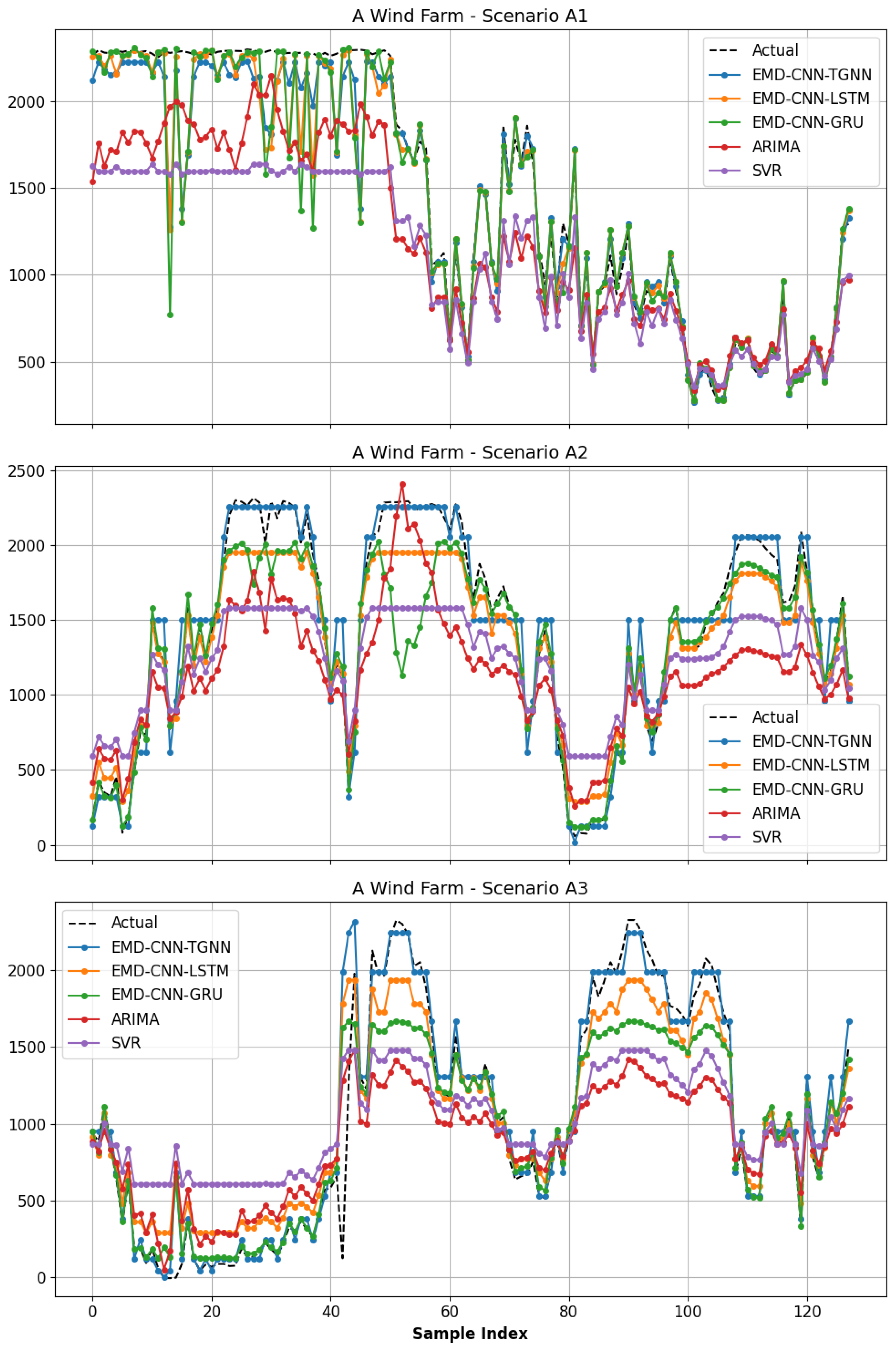
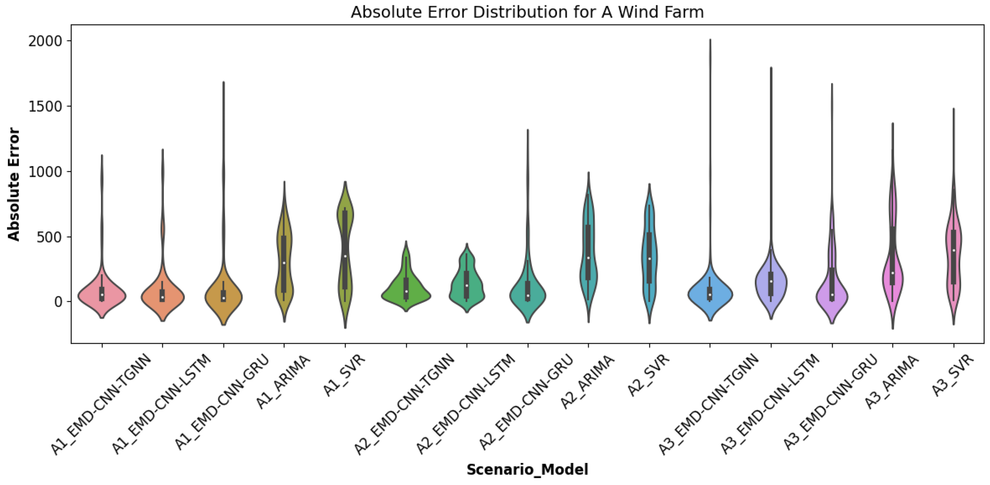
• In Wind Farm A, the TGNN model (EMD–CNN–TGNN) demonstrated higher predictive accuracy for turbines A1, A2, and A3, especially in capturing rapid fluctuations in the data more closely. Compared to EMD–CNN–LSTM and EMD–CNN–GRU, which exhibited varying degrees of deviation, ARIMA and SVR performed the poorest, underscoring the TGNN model’s superior ability to capture complex patterns and trends in the data.
• Against EMD–CNN–LSTM, the TGNN model showed improvements of 7.88% in MAE, 26.09% in MSE, 14.03% in RMSE, and an increase of 3.30% in $R^2$. Compared to EMD–CNN–GRU and particularly SVR, the differences were even more pronounced, with an up to 56.67% improvement in $R^2$ with SVR, highlighting the TGNN model’s significant advantages in prediction accuracy and data fitting.
• In the data for turbines A2 and A3, the TGNN model continued to show higher performance enhancements, notably against ARIMA in turbine A2 data, where the improvement in $R^2$ reached an impressive 66.67%, further proving the TGNN model’s excellence in complex data settings.
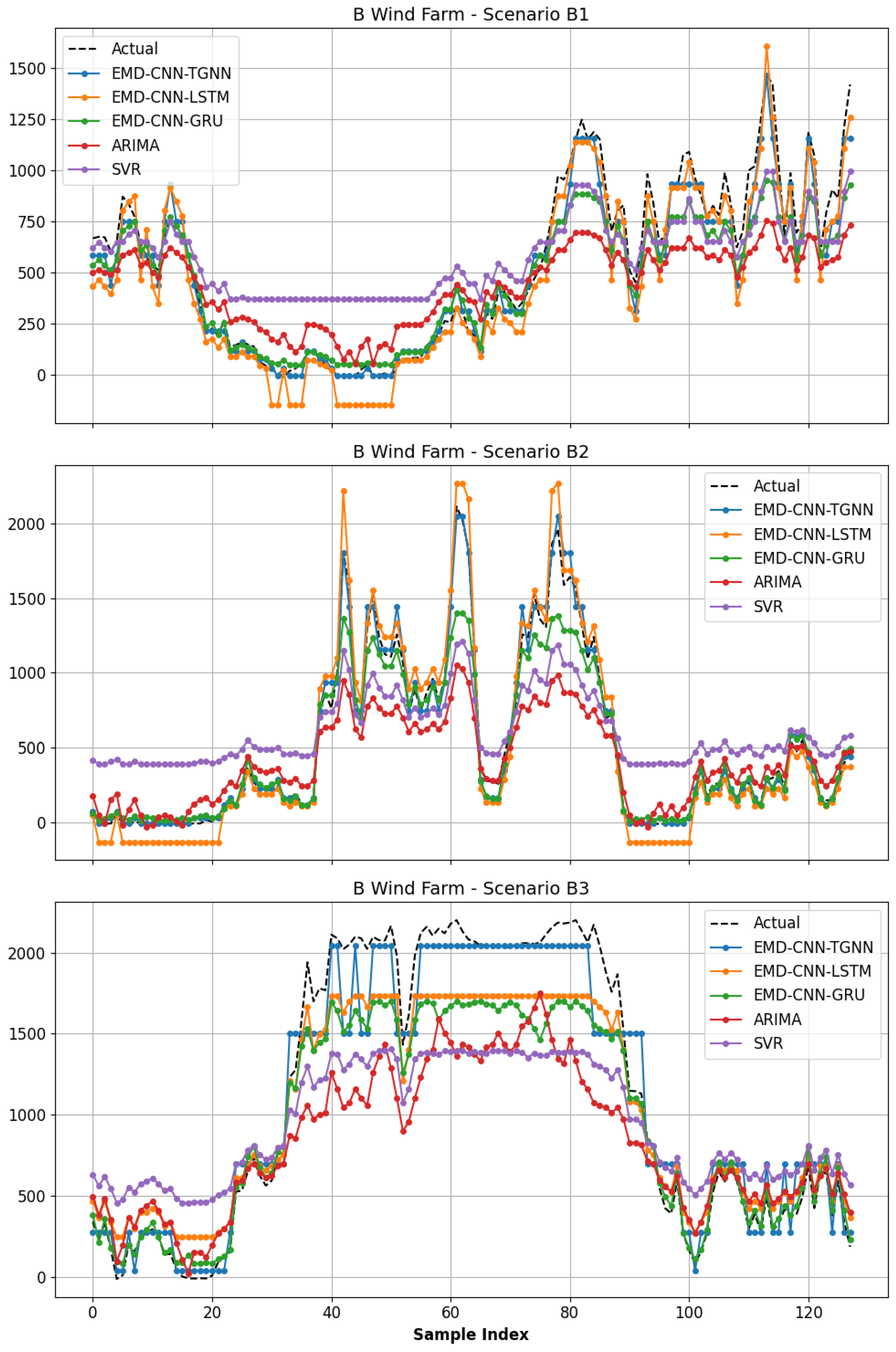
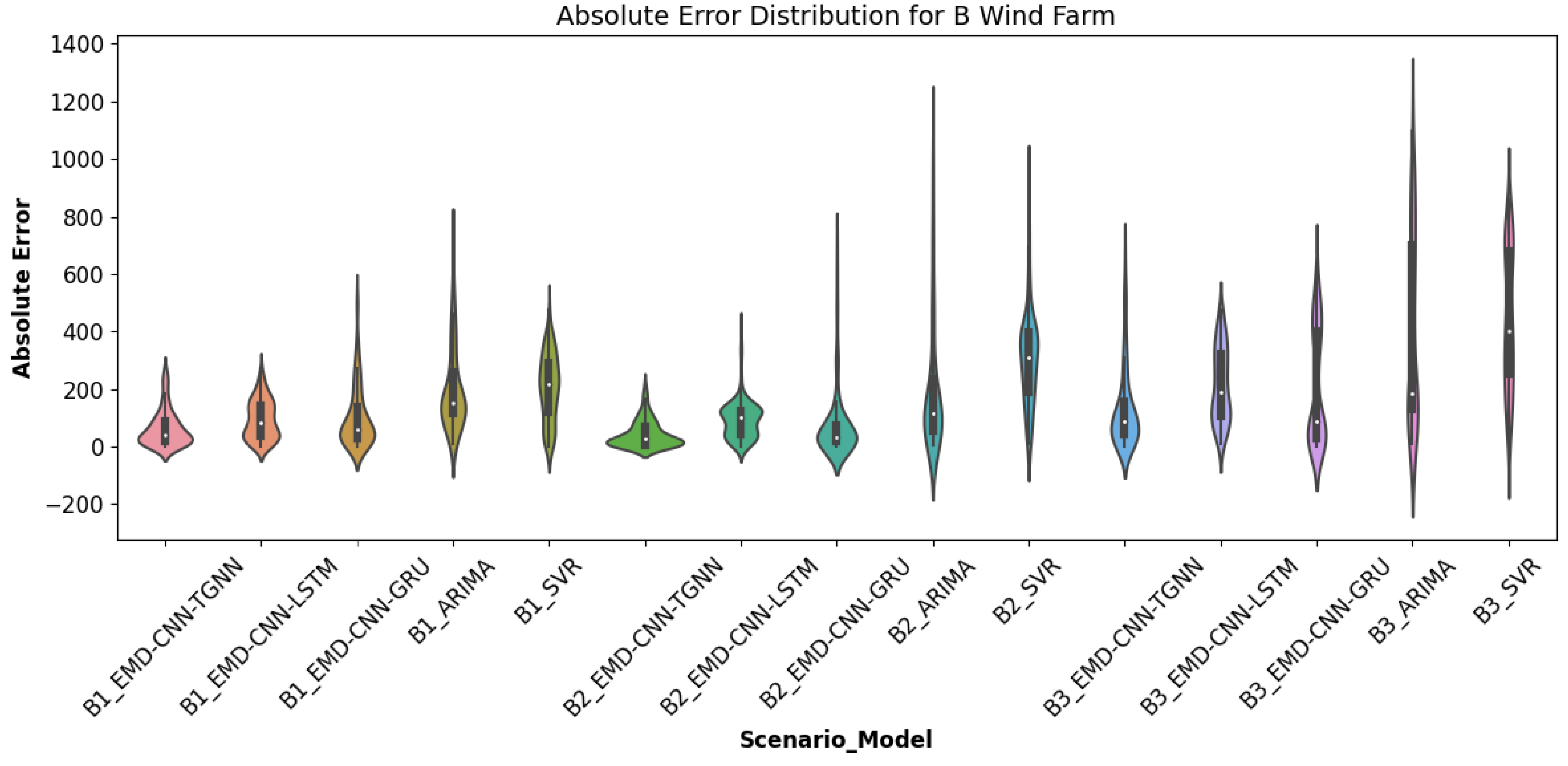
• In Wind Farm B, the performance of the five models varied across turbines B1, B2, and B3. Notably, in turbine B1 data, the EMD–CNN–LSTM improved and approached the actual data more closely. However, the EMD–CNN–TGNN maintained consistency and stability overall, especially in turbine B2 data, where its predictive path highly aligned with the actual wind power outputs. The TGNN model also exhibited superior performance, particularly in turbine B2 data compared to SVR, with a 59.68% improvement in $R^2$ and a 3.26% increase over the well-performing EMD–CNN–LSTM in turbine B1 data, indicating the TGNN model’s enhanced accuracy and reliability across different turbine data scenarios.
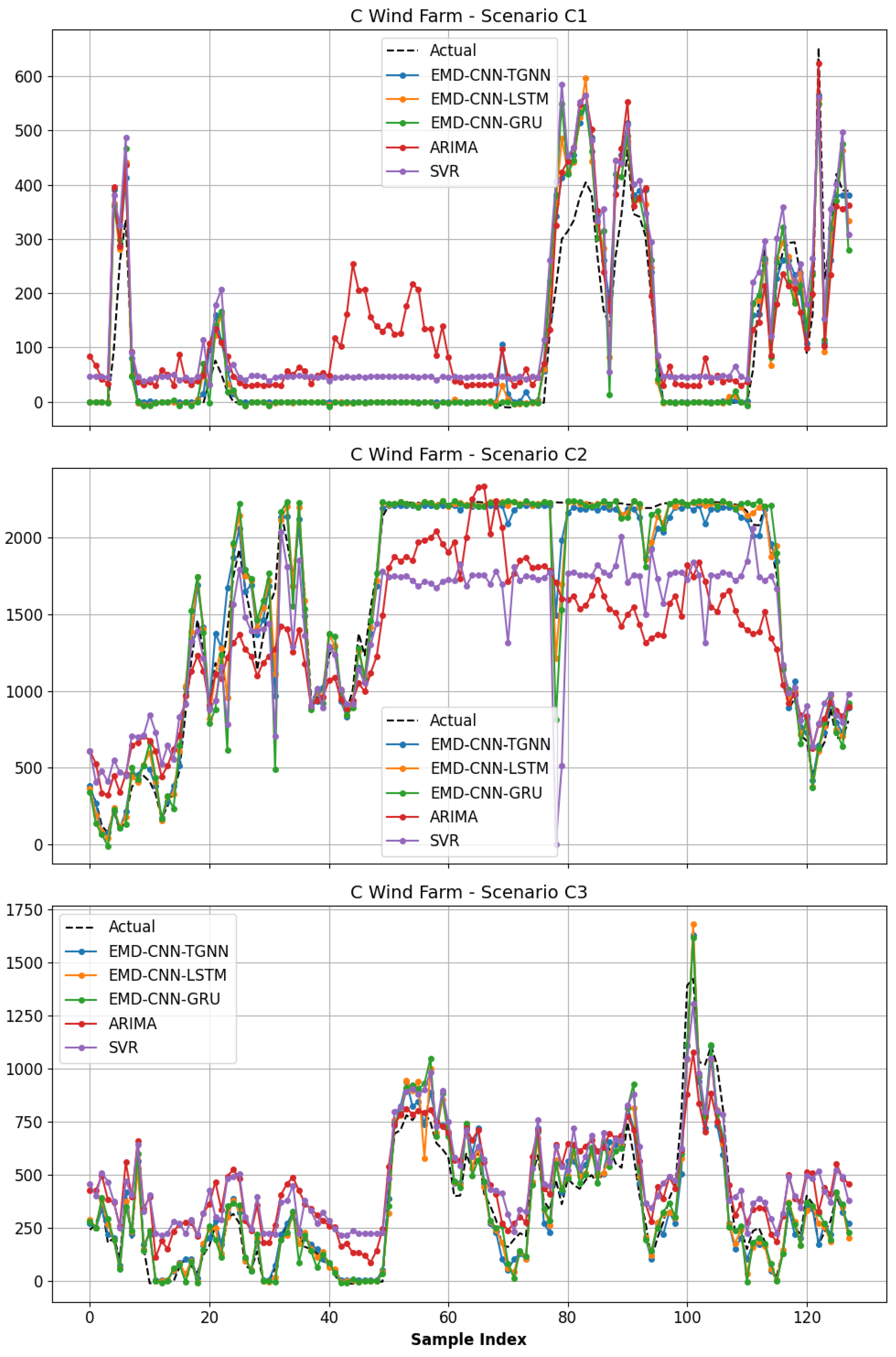
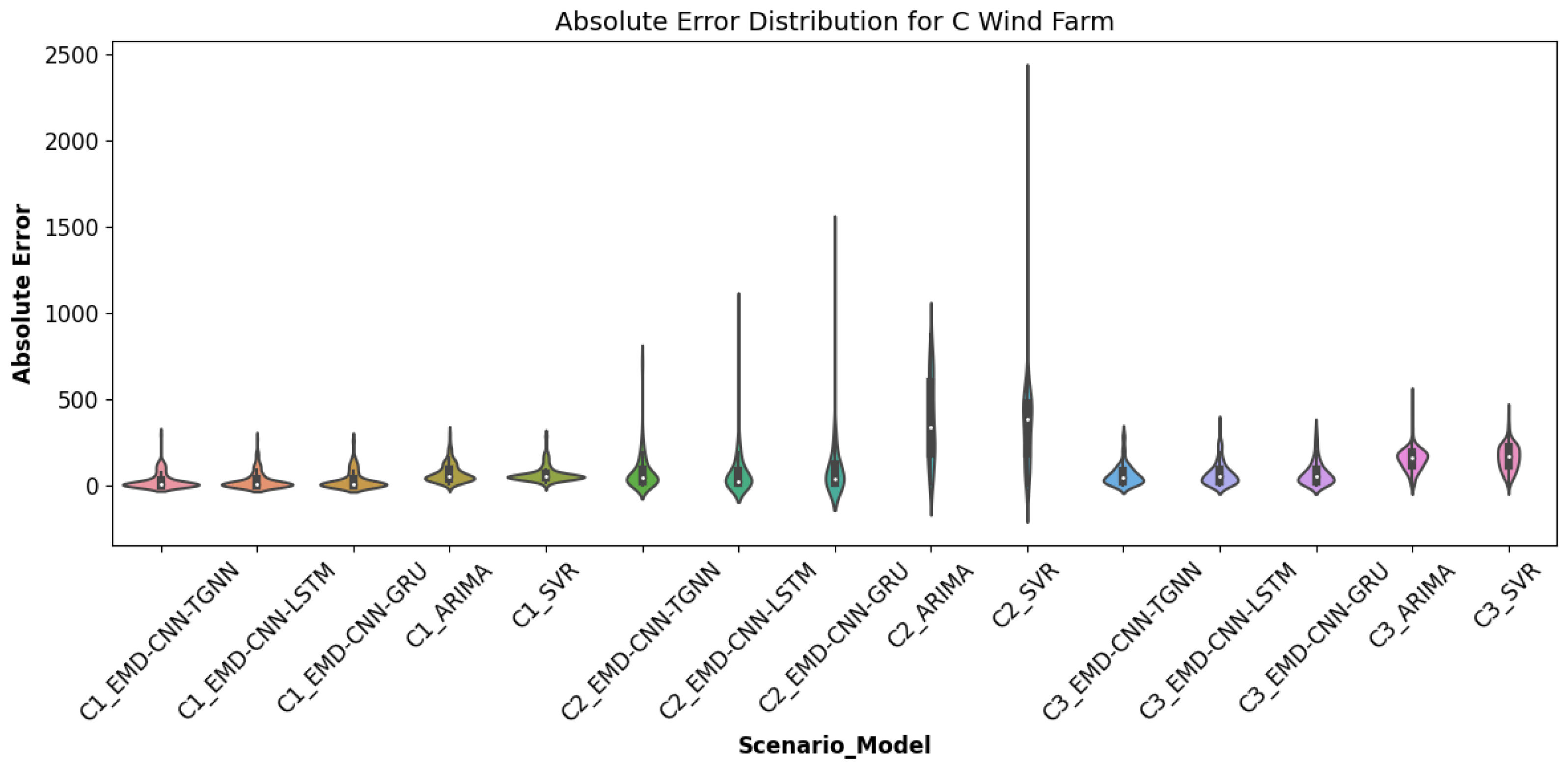
• In Wind Farm C, the EMD–CNN–TGNN maintained good performance in capturing rapid changes, while the EMD–CNN–GRU showed weaker performance in sudden shifts, and ARIMA and SVR lagged significantly behind the other three models. The performance of EMD–CNN–TGNN in Wind Farm C emphasizes its robustness against disturbances during abrupt events. Compared to other models, especially in turbine C2 data against SVR, the increase in $R^2$ reached 61.67%, demonstrating its strong capability in capturing data trends and fluctuations. In turbine C1 data, the TGNN model increased $R^2$ by 45.00% compared to ARIMA, further highlighting its accuracy across different wind power data scenarios.

Table 8. Average model prediction performance at Wind Farm A.

Model	MAE (kw)	MSE (kw)	RMSE (kw)	${\mathit{R}}^2$
EMD–CNN–TGNN	98.54	34,174.33	182.95	0.93
EMD–CNN–LSTM	134.28	45,521.78	211.65	0.91
EMD–CNN–GRU	132.61	67,208.28	259.11	0.87
ARIMA	339.45	173,620.88	415.49	0.65
SVR	365.94	193,205.82	438.91	0.62

,

Table 9. Average model prediction performance at Wind Farm B.

Model	MAE (kw)	MSE (kw)	RMSE (kw)	${\mathit{R}}^2$
EMD–CNN–TGNN	80.80	16,756.76	116.71	0.96
EMD–CNN–LSTM	135.75	30,190.36	161.95	0.93
EMD–CNN–GRU	130.00	42,401.49	196.13	0.89
ARIMA	270.33	144,513.07	363.60	0.63
SVR	319.13	143,387.66	362.67	0.64

,

Table 10. Average model prediction performance at Wind Farm C.

Model	MAE (kw)	MSE (kw)	RMSE (kw)	${\mathit{R}}^2$
EMD–CNN–TGNN	54.44	8982.16	89.43	0.92
EMD–CNN–LSTM	57.46	11,548.18	100.39	0.90
EMD–CNN–GRU	67.65	20,124.73	124.92	0.87
ARIMA	199.39	77,858.37	234.00	0.63
SVR	196.69	83,264.56	239.07	0.64

,

Table 11. EMD–CNN–TGNN average performance improvement at Wind Farm A.

Comparison	MAE (%)	MSE (%)	RMSE (%)	${\mathit{R}}^2$ (%)
EMD–CNN–TGNN vs. EMD–CNN–LSTM	23.95	25.60	13.76	2.56
EMD–CNN–TGNN vs. EMD–CNN–GRU	24.01	49.85	29.65	7.70
EMD–CNN–TGNN vs. ARIMA	70.94	79.75	55.63	44.42
EMD–CNN–TGNN vs. SVR	72.94	82.40	58.38	51.45

,

Table 12. EMD–CNN–TGNN average performance improvement at Wind Farm B.

Comparison	MAE (%)	MSE (%)	RMSE (%)	${\mathit{R}}^2$ (%)
EMD–CNN–TGNN vs. EMD–CNN–LSTM	41.23	49.53	29.86	3.59
EMD–CNN–TGNN vs. EMD–CNN–GRU	39.32	66.45	43.07	8.29
EMD–CNN–TGNN vs. ARIMA	71.10	89.51	68.66	52.24
EMD–CNN–TGNN vs. SVR	74.64	88.89	68.06	51.42

and

Table 13. EMD–CNN–TGNN average performance improvement at Wind Farm C.

Comparison	MAE (%)	MSE (%)	RMSE (%)	${\mathit{R}}^2$ (%)
EMD–CNN–TGNN vs. EMD–CNN–LSTM	5.91	18.71	9.89	2.29
EMD–CNN–TGNN vs. EMD–CNN–GRU	17.56	36.28	21.38	4.98
EMD–CNN–TGNN vs. ARIMA	67.66	76.91	53.62	45.62
EMD–CNN–TGNN vs. SVR	67.07	75.11	52.48	44.68

are employed to evaluate the comprehensive predictive performance of the EMD–CNN–TGNN model across all datasets and compare it with other models including EMD–CNN–LSTM, EMD–CNN–GRU, ARIMA, and SVR. The EMD–CNN–TGNN model showcases leading performance across all major metrics, achieving the lowest mean absolute error (MAE = 77.93), mean squared error (MSE = 19,971.08), root mean squared error (RMSE = 129.70), and the highest coefficient of determination ($R^2=0.94$). These results demonstrate the superiority of EMD–CNN–TGNN in both prediction accuracy and data fit over the competing models.

The EMD–CNN–LSTM and EMD–CNN–GRU models, while superior to ARIMA and SVR, do not match the performance of EMD–CNN–TGNN. Specifically, the $R^2$ values for EMD–CNN–LSTM and EMD–CNN–GRU are 0.91 and 0.88, respectively, indicating a lesser ability to explain variability in the data. ARIMA and SVR significantly under-perform across all metrics, particularly in MSE and RMSE, reflecting their limitations in handling wind power prediction tasks. Their respective $R^2$ values of 0.64 and 0.63 highlight substantial disparities in data fitting.

Relative to EMD–CNN–LSTM, EMD–CNN–TGNN exhibits performance improvements of 23.70% in MAE, 31.28% in MSE, and 17.84% in RMSE, with a 2.82% increase in $R^2$. These enhancements emphasize the significant accuracy gains provided by EMD–CNN–TGNN. Against EMD–CNN–GRU, the improvements are even more pronounced, especially in MSE and RMSE, the values of which are higher by 50.86% and 31.36%, respectively, with a 6.99% increase in $R^2$.

Compared with ARIMA and SVR, EMD–CNN–TGNN not only shows substantial improvements in MAE, MSE, and RMSE (exceeding 69.90% and 71.55%, respectively), but also demonstrates remarkable increases in $R^2$ of 47.43% and 49.18%, respectively. These comparisons highlight the exceptional ability of EMD–CNN–TGNN to predict wind power time series data with high data fitting accuracy.

Based on the comprehensive performance comparison facilitated by

Table 14. Overall average performance of each model.

Model	MAE (kw)	MSE (kw)	RMSE (kw)	${\mathit{R}}^2$
EMD–CNN–TGNN	77.93	19,971.08	129.70	0.94
EMD–CNN–LSTM	109.16	29,086.77	157.99	0.91
EMD–CNN–GRU	110.09	43,244.83	193.39	0.88
ARIMA	269.72	131,997.44	337.70	0.64
SVR	293.92	139,952.68	346.88	0.63

and

Table 15. Average performance improvement of EMD–CNN–TGNN across all datasets.

Comparison (Model 1 vs. Model)	MAE (%)	MSE (%)	RMSE (%)	${\mathit{R}}^2$ (%)
EMD–CNN–TGNN vs. EMD–CNN–LSTM	23.70	31.28	17.84	2.82
EMD–CNN–TGNN vs. EMD–CNN–GRU	26.96	50.86	31.36	6.99
EMD–CNN–TGNN vs. ARIMA	69.90	82.06	59.30	47.43
EMD–CNN–TGNN vs. SVR	71.55	82.13	59.64	49.18

, and a detailed analysis of performance enhancements, it is observed that the EMD–CNN–TGNN model achieved significant improvements in key metrics such as MAE, MSE, RMSE, and $R^2$. Specifically, compared to the EMD–CNN–GRU and EMD–CNN–LSTM models, EMD–CNN–TGNN exhibited an average performance enhancement of 23.68% in MAE, 28.85% in MSE, 17.83% in RMSE, and 2.81% in $R^2$. Moreover, when compared against the EMD–CNN–LSTM model, there were further increases of 28.49%, 65.66%, 34.84%, and 6.89%, respectively. The performance uplift was even more pronounced when contrasted with traditional models such as ARIMA and SVR, which showed improvements of 69.90%, 82.06%, 59.30%, 47.43%, and 71.55%, 82.13%, 59.64%, 49.18%, respectively.

These performance metrics not only validate the significant advantages of the EMD–CNN–TGNN model over existing models but also provide vital references and foundations for future research directions and applications. The following sections outline the implications of these findings and suggest areas for further investigation.

5. Conclusions and Discussions

In summary, a novel hybrid model named EMD–CNN–TGNN has been proposed to enhance the accuracy of short-term wind power forecasting. Within this hybrid model, the empirical mode decomposition (EMD) algorithm effectively reduces the volatility of wind speed series, the convolutional neural network (CNN) efficiently extracts features from wind power data, and the three-dimensional gated neural network (TGNN) utilizes its tri-gate characteristics to effectively predict based on these features. The EMD–CNN–TGNN model demonstrates superior average performance with an MAE of 54.44, MSE of 8982.16, RMSE of 89.43, and $R^2$ of 0.92, surpassing the other two hybrid models and two traditional models.

Considering the enhanced accuracy of the proposed EMD–CNN–TGNN model, it implies significant benefits for wind farm operational management. More accurate power output predictions can optimize electricity dispatch and energy management strategies, thereby reducing economic losses due to forecasting errors. Additionally, this model could be applied to the energy storage systems of wind farms, providing forecast data to the control systems of PEM electrolyzers to adjust their efficiency curves and improve the utilization rate of wind energy.

Despite the high performance demonstrated by the TGNN in experiments, its structural complexity and the need for parameter tuning may pose challenges in practical deployments. Balancing the improvement in prediction accuracy with the simplification of model complexity is a critical consideration for future research. Further studies could explore more efficient training techniques, such as knowledge distillation or model pruning, and the use of lightweight network architectures to reduce computational resource consumption. These techniques will be explored in subsequent research to provide guidance for the practical deployment of the model.

References

1. Wang, H.-z.; Li, G.-q.; Wang, G.-b.; Peng, J.-c.; Jiang, H.; Liu, Y.-t. Deep learning based ensemble approach for probabilistic wind power forecasting. Appl. Energy 2017, 188, 56–70. [Google Scholar] [CrossRef]
2. Vargas, S.A.; Esteves, G.R.T.; Maçaira, P.M.; Bastos, B.Q.; Cyrino Oliveira, F.L.; Souza, R.C. Wind power generation: A review and a research agenda. J. Clean. Prod. 2019, 218, 850–870. [Google Scholar] [CrossRef]
3. Hassan, Q.; Algburi, S.; Sameen, A.Z.; Salman, H.M.; Jaszczur, M. A review of hybrid renewable energy systems: Solar and wind-powered solutions: Challenges, opportunities, and policy implications. Results Eng. 2023, 20, 101621. [Google Scholar] [CrossRef]
4. Petersen, C.; Reguant, M.; Segura, L. Measuring the impact of wind power and intermittency. Energy Econ. 2024, 129, 107200. [Google Scholar] [CrossRef]
5. Rumelhart, D.E.; Hinton, G.E.; Williams, R.J. Learning representations by back-propagating errors. Nature 1986, 323, 533–536. [Google Scholar] [CrossRef]
6. Hochreiter, S.; Schmidhuber, J. Long Short-Term Memory. Neural Comput. 1997, 9, 1735–1780. [Google Scholar] [CrossRef] [PubMed]
7. Cho, K.; Van Merriënboer, B.; Gulcehre, C.; Bahdanau, D.; Bougares, F.; Schwenk, H.; Bengio, Y. Learning phrase representations using RNN encoder-decoder for statistical machine translation. arXiv 2014, arXiv:1406.1078. [Google Scholar]
8. Prema, V.; Bhaskar, M.S.; Almakhles, D.; Gowtham, N.; Rao, K.U. Critical review of data, models and performance metrics for wind and solar power forecast. IEEE Access 2021, 10, 667–688. [Google Scholar] [CrossRef]
9. Shahid, F.; Zameer, A.; Muneeb, M. A novel genetic LSTM model for wind power forecast. Energy 2021, 223, 120069. [Google Scholar] [CrossRef]
10. Xiang, L.; Liu, J.; Yang, X.; Hu, A.; Su, H. Ultra-short term wind power prediction applying a novel model named SATCN-LSTM. Energy Convers. Manag. 2022, 252, 115036. [Google Scholar] [CrossRef]
11. Cui, Y.; Chen, Z.; He, Y.; Xiong, X.; Li, F. An algorithm for forecasting day-ahead wind power via novel long short-term memory and wind power ramp events. Energy 2023, 263, 125888. [Google Scholar] [CrossRef]
12. Kisvari, A.; Lin, Z.; Liu, X. Wind power forecasting—A data-driven method along with gated recurrent neural network. Renew. Energy 2021, 163, 1895–1909. [Google Scholar] [CrossRef]
13. Liu, X.; Yang, L.; Zhang, Z. Short-Term Multi-Step Ahead Wind Power Predictions Based On A Novel Deep Convolutional Recurrent Network Method. IEEE Trans. Sustain. Energy 2021, 12, 1820–1833. [Google Scholar] [CrossRef]
14. Xiao, Y.; Zou, C.; Chi, H.; Fang, R. Boosted GRU model for short-term forecasting of wind power with feature-weighted principal component analysis. Energy 2022, 267, 126503. [Google Scholar] [CrossRef]
15. Masoumi, M. Machine Learning Solutions for Offshore Wind Farms: A Review of Applications and Impacts. J. Mar. Sci. Eng. 2023, 11, 1855. [Google Scholar] [CrossRef]
16. Kontopoulou, V.I.; Panagopoulos, A.; Kakkos, I.; Matsopoulos, G. A Review of ARIMA vs. Machine Learning Approaches for Time Series Forecasting in Data Driven Networks. Future Internet 2023, 15, 255. [Google Scholar] [CrossRef]
17. de Moraes Vieira, J.L.; Farias, F.C.; Ochoa, A.A.V.; de Menezes, F.D.; da Costa, A.C.A.; Ângelo Peixoto da Costa, J.; de Novaes Pires Leite, G.; de Castro Vilela, O.; de Souza, M.G.G.; Michima, P. Remaining Useful Life Estimation Framework for the Main Bearing of Wind Turbines Operating in Real Time. Energies 2024, 17, 1430. [Google Scholar] [CrossRef]
18. Chicco, D.; Warrens, M.J.; Jurman, G. The coefficient of determination R-squared is more informative than SMAPE, MAE, MAPE, MSE and RMSE in regression analysis evaluation. Peerj Comput. Sci. 2021, 7, e623. [Google Scholar] [CrossRef] [PubMed]
19. Bokde, N.; Feijóo, A.; Villanueva, D.; Kulat, K. A review on hybrid empirical mode decomposition models for wind speed and wind power prediction. Energies 2019, 12, 254. [Google Scholar] [CrossRef]
20. Liang, H.; Bressler, S.L.; Desimone, R.; Fries, P. Empirical mode decomposition: A method for analyzing neural data. Neurocomputing 2005, 65, 801–807. [Google Scholar] [CrossRef]
21. Khaldi, R.; El Afia, A.; Chiheb, R.; Tabik, S. What is the best RNN-cell structure to forecast each time series behavior? Expert Syst. Appl. 2023, 215, 119140. [Google Scholar] [CrossRef]
22. Triguero, I.; García-Gil, D.; Maillo, J.; Luengo, J.; García, S.; Herrera, F. Transforming big data into smart data: An insight on the use of the k-nearest neighbors algorithm to obtain quality data. Wiley Interdiscip. Rev. Data Min. Knowl. Discov. 2019, 9, e1289. [Google Scholar] [CrossRef]
23. Urolagin, S.; Sharma, N.; Datta, T.K. A combined architecture of multivariate LSTM with Mahalanobis and Z-Score transformations for oil price forecasting. Energy 2021, 231, 120963. [Google Scholar] [CrossRef]
24. Khosravi, A.; Machado, L.; Nunes, R. Time-series prediction of wind speed using machine learning algorithms: A case study Osorio wind farm, Brazil. Appl. Energy 2018, 224, 550–566. [Google Scholar] [CrossRef]
25. Zhao, Z.; Yun, S.; Jia, L.; Guo, J.; Meng, Y.; He, N.; Li, X.; Shi, J.; Yang, L. Hybrid VMD-CNN-GRU-based model for short-term forecasting of wind power considering spatio-temporal features. Eng. Appl. Artif. Intell. 2023, 121, 105982. [Google Scholar] [CrossRef]
Figure 1. Geographic locations of wind farms.
Sustainability 16 03474 g001
Figure 2. EMD –CNN–TGNN structure diagram.
Sustainability 16 03474 g002
Figure 3. EMDestablishment matrix diagram.
Sustainability 16 03474 g003
Figure 4. TGNN layer structure diagram.
Sustainability 16 03474 g004
Figure 5. TGNE diagram (three-dimensional gated neural elements diagram).
Sustainability 16 03474 g005
Figure 6. Flowchart of implementation steps.
Sustainability 16 03474 g006
Figure 7. Comparison of model predictions with actual values for three turbines at Wind Farm A.
Sustainability 16 03474 g007
Figure 8. Comparison of model predictions with actual values for three turbines at Wind Farm B.
Sustainability 16 03474 g008
Figure 9. Comparison of model predictions with actual values for three turbines at Wind Farm C.
Sustainability 16 03474 g009
Figure 10. Violin plot of prediction errors for various models at Wind Farm A.
Sustainability 16 03474 g010
Figure 11. Violin plot of prediction errors for various models at Wind Farm B.
Sustainability 16 03474 g011
Figure 12. Violin plot of prediction errors for various models at Wind Farm C.
Sustainability 16 03474 g012