Multi-Model Comprehensive Inversion of Surface Soil Moisture from Landsat Images Based on Machine Learning Algorithms

Abstract
:1. Introduction
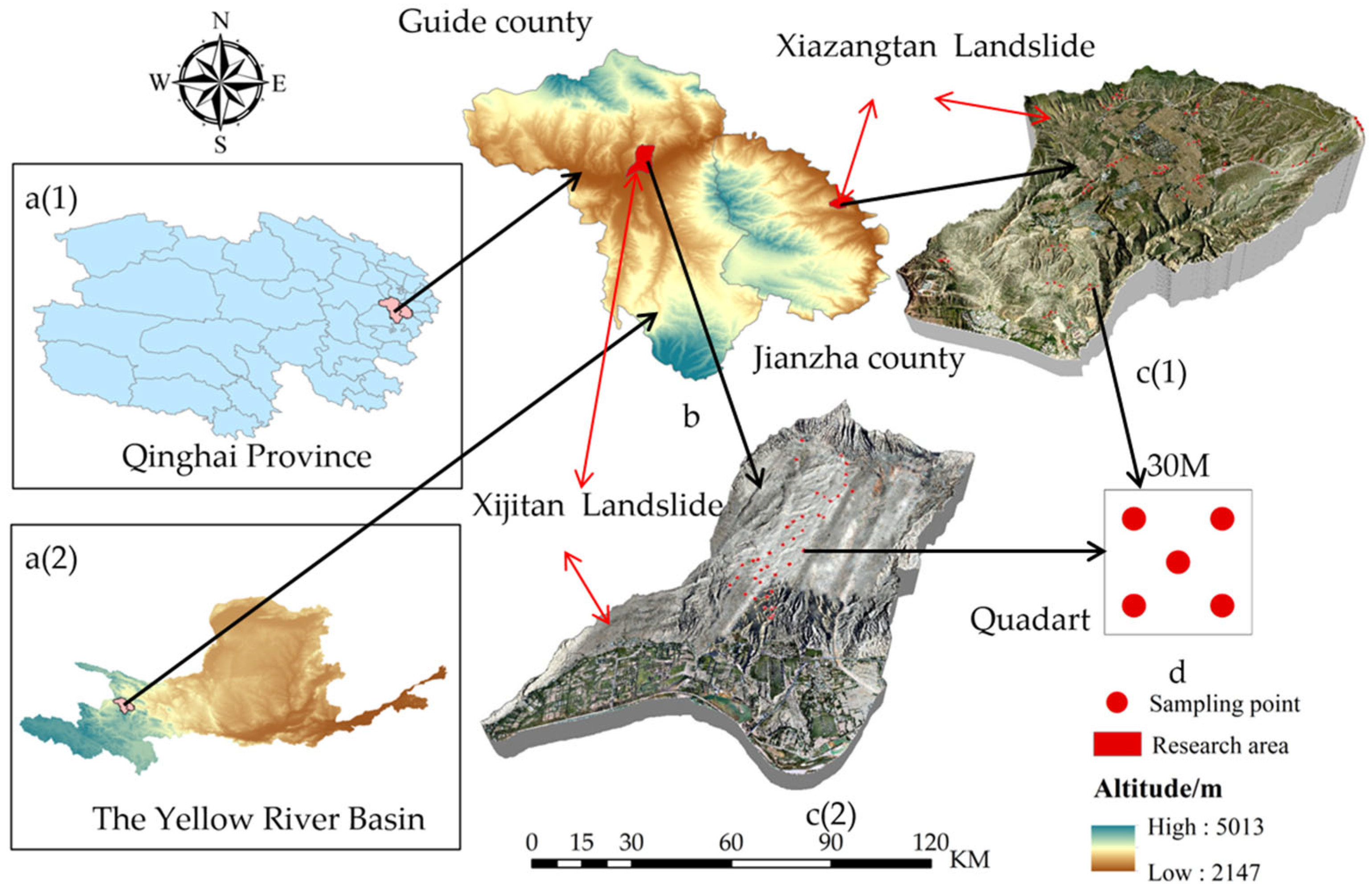
2. Study Area
3. Materials and Methods
3.1. Data
3.1.1. In Situ Soil Moisture Data
3.1.2. Remote Sensing Data
3.2. Environmental Variables and Surface Temperature Calculations
3.2.1. Derivation of Environmental Variables
3.2.2. Surface Temperature
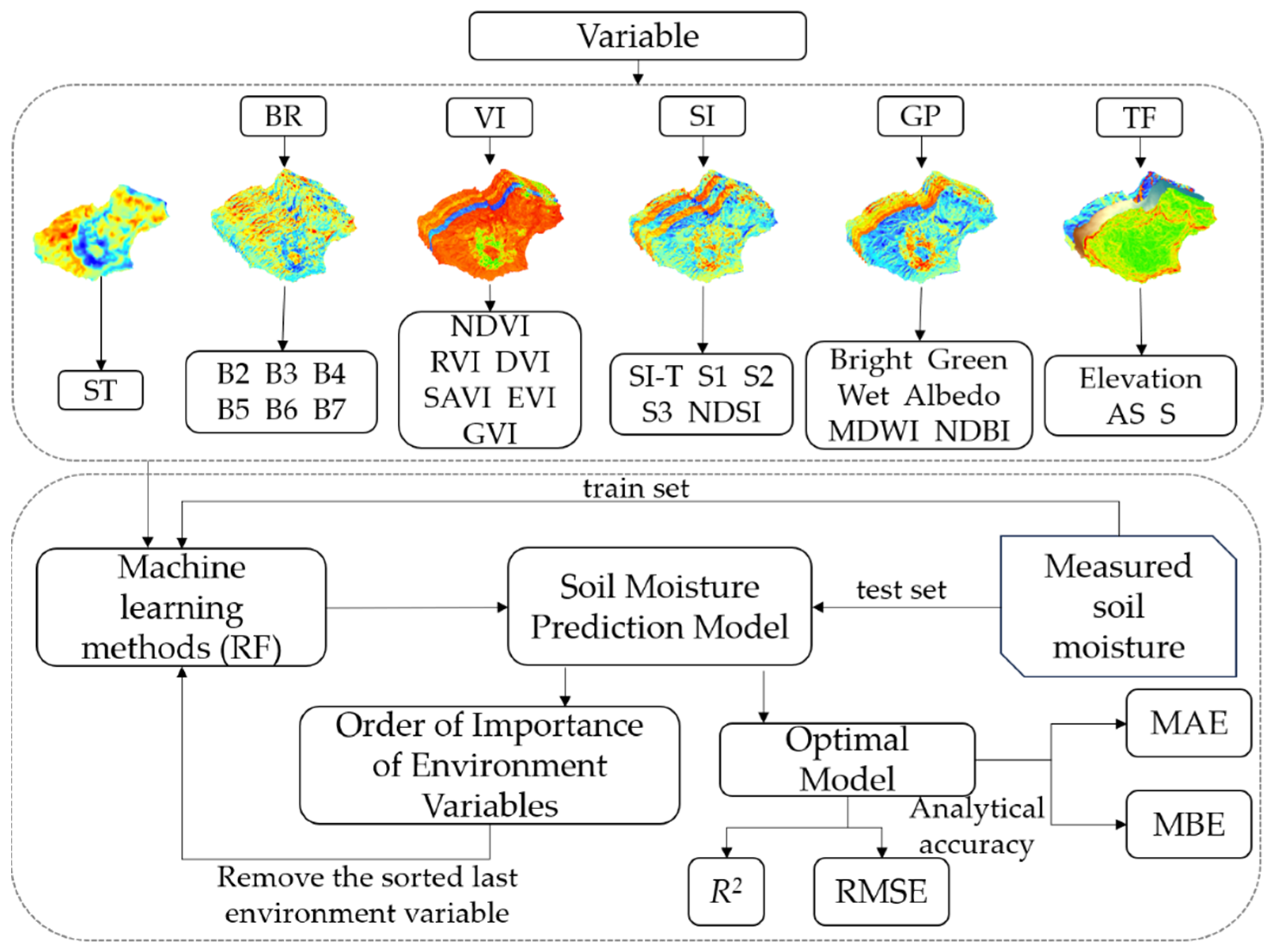
3.3. Variable Preference
3.4. Modeling Methodology
3.4.1. Random Forest (RF) Model
3.4.2. Support Vector Machine (SVM) Model
3.4.3. Back Propagation Neural Network (BPNN) Model
3.4.4. Combined Model
3.5. Model Construction and Validation
4. Results
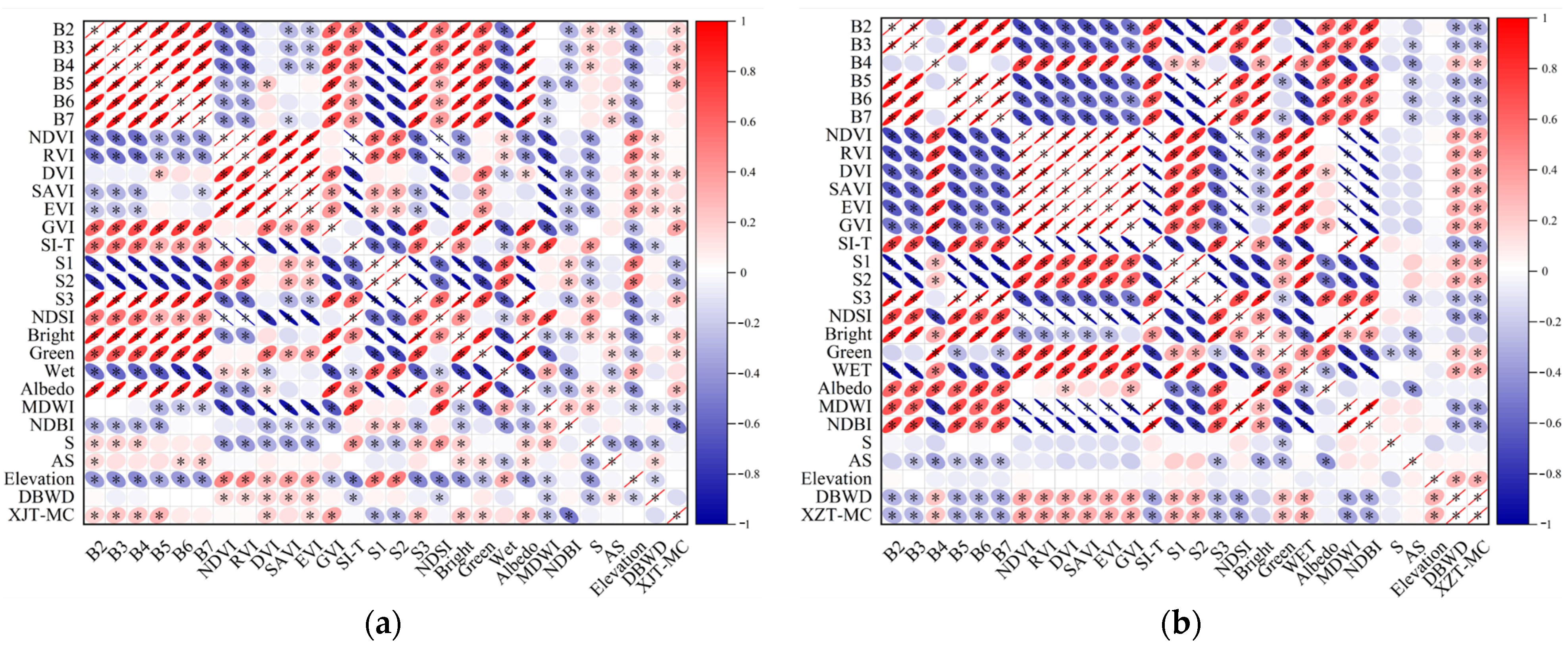
4.1. Correlation between Environmental Variables and Surface Soil Moisture
4.2. Importance of Environmental Variables and Optimal Independent Variable Sets
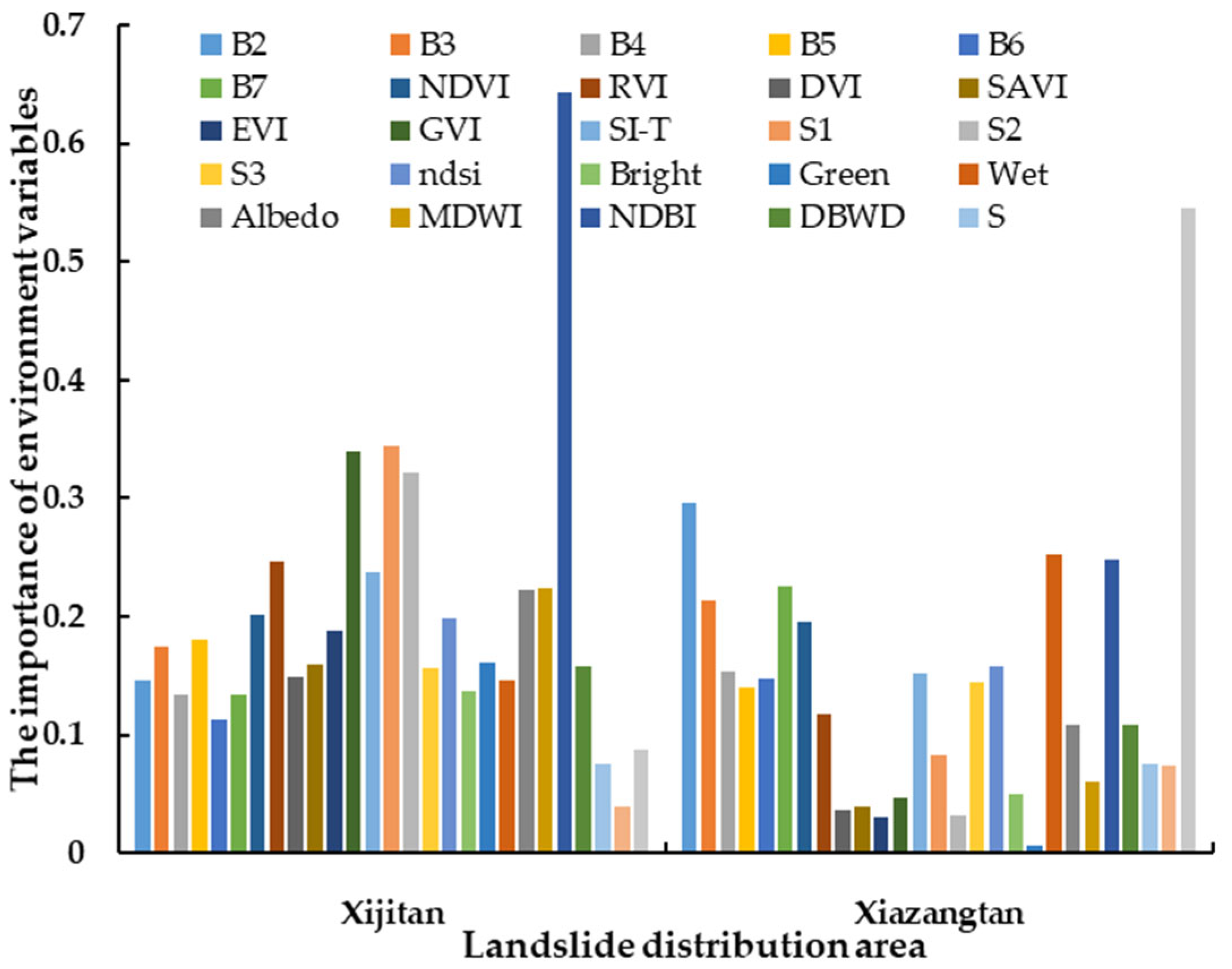
4.2.1. Importance of Environmental Variables
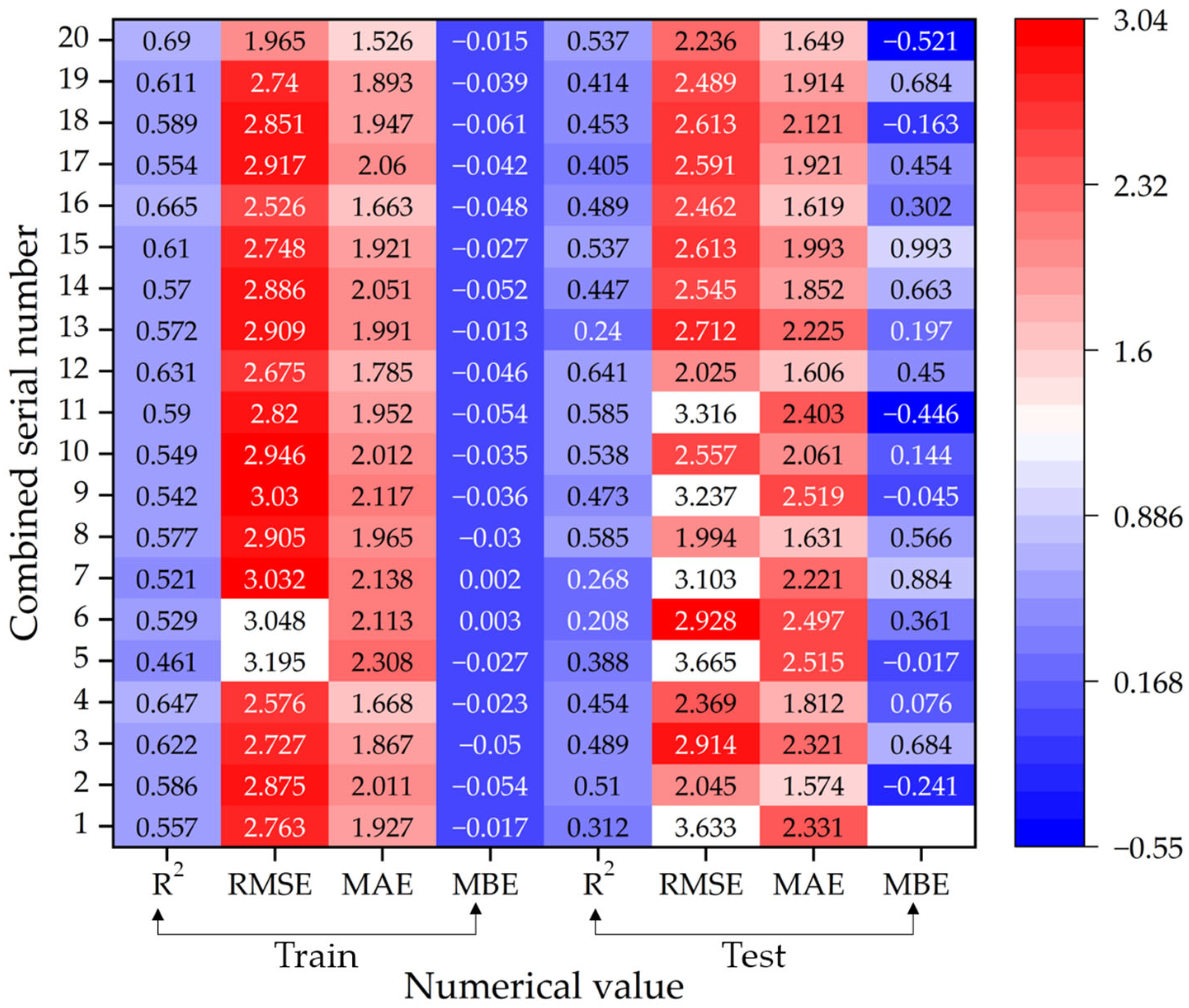
4.2.2. Screening for Optimal Combinations of Independent Variables
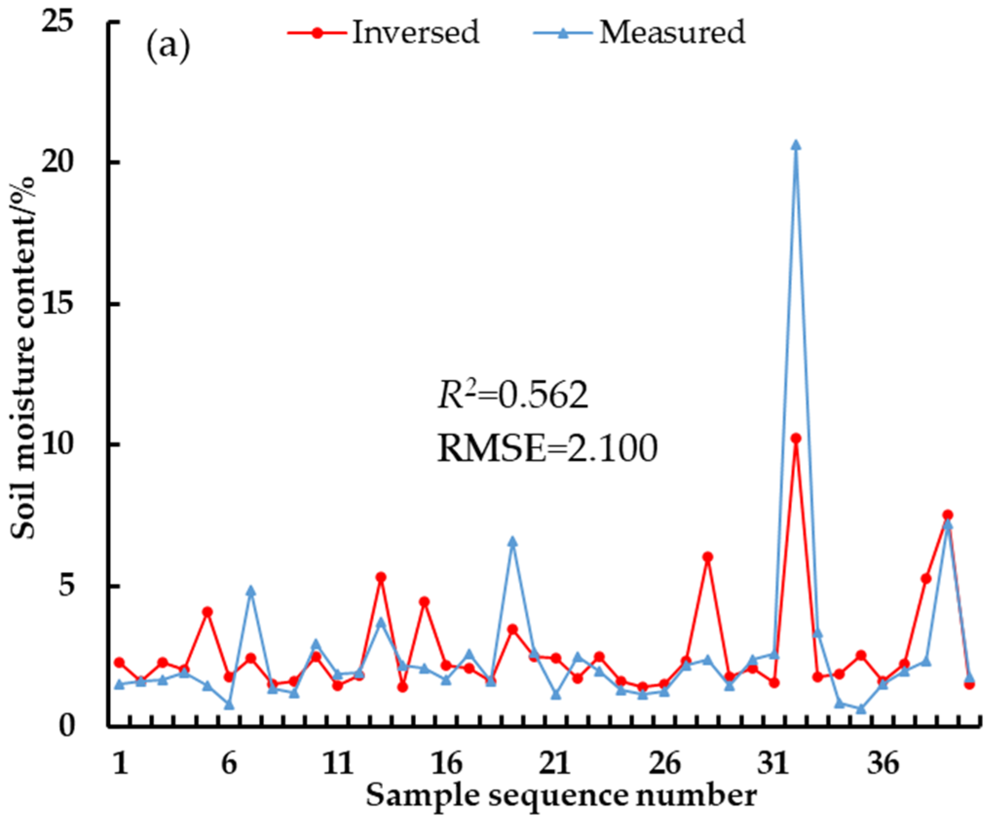
4.3. Predicted Soil Moisture in Different Areas
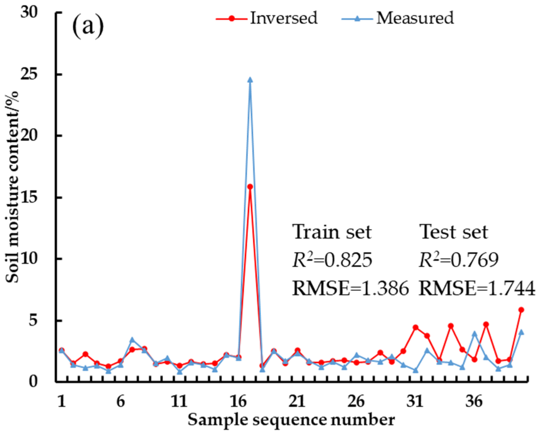
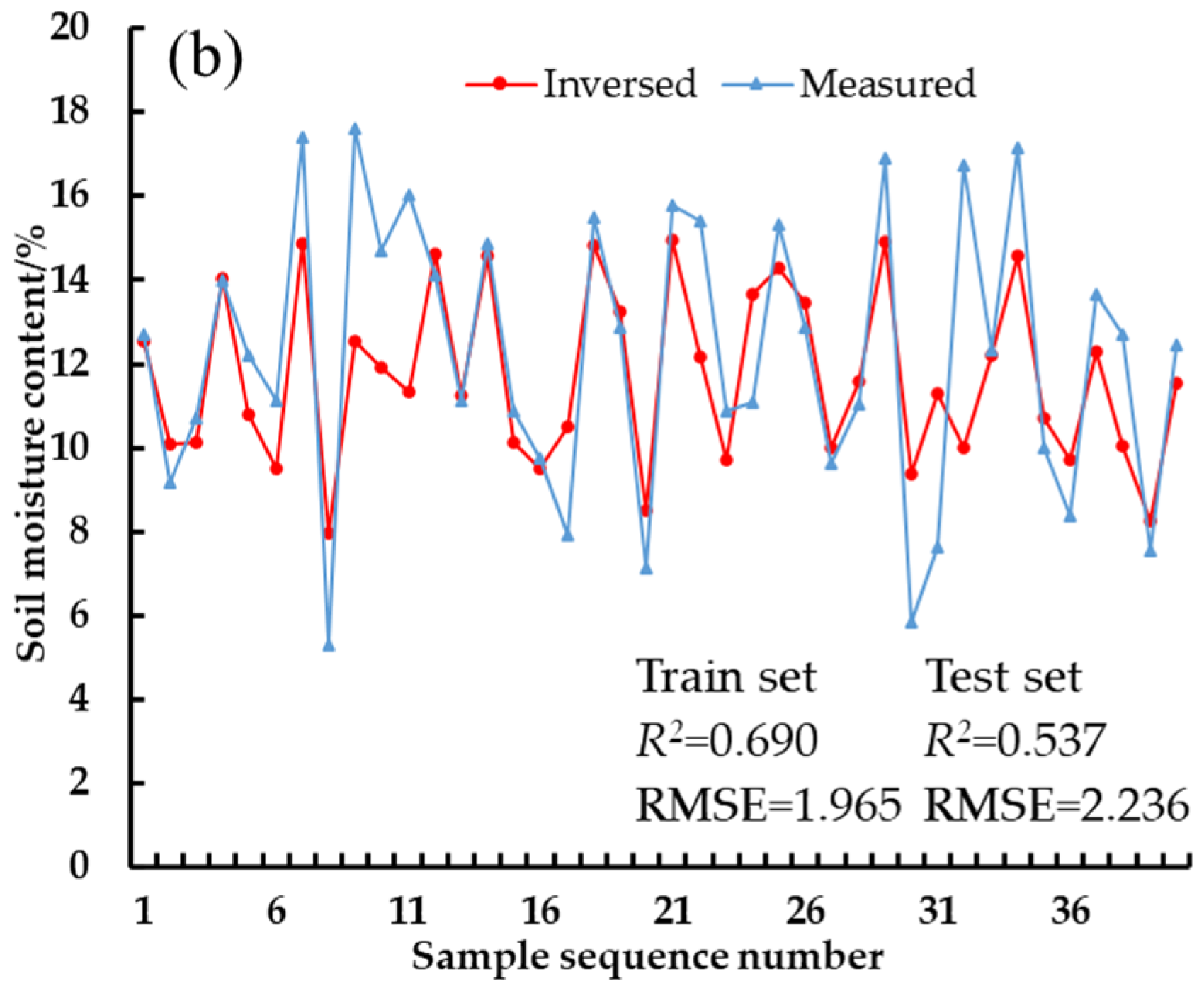
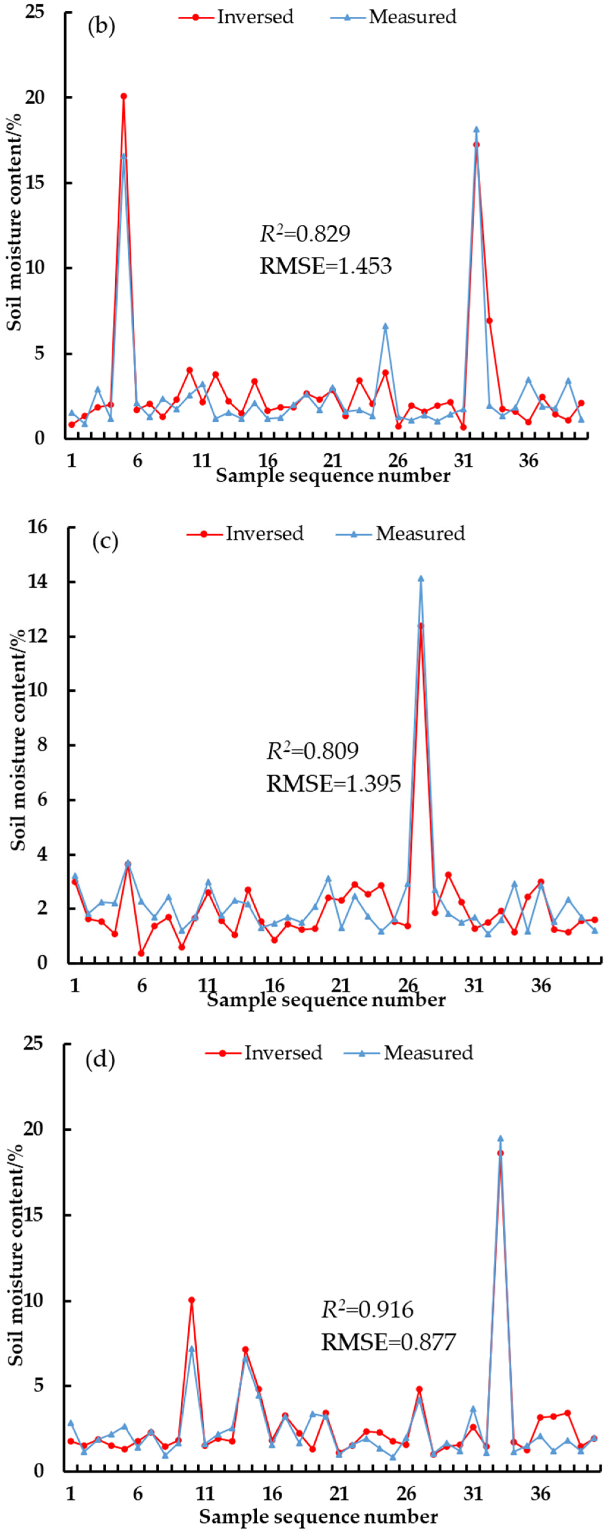
4.4. Model Construction and Validation of Different Methods
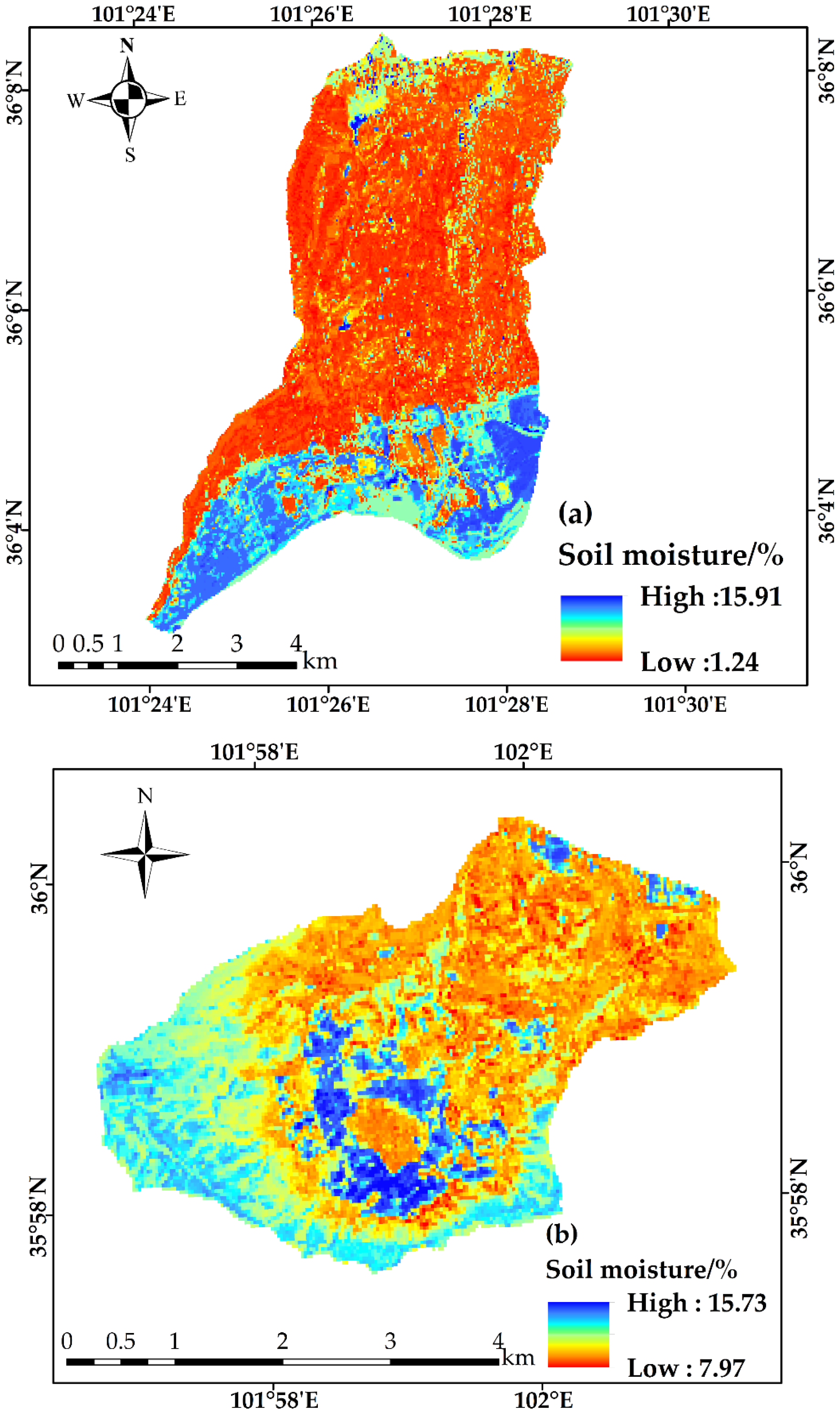
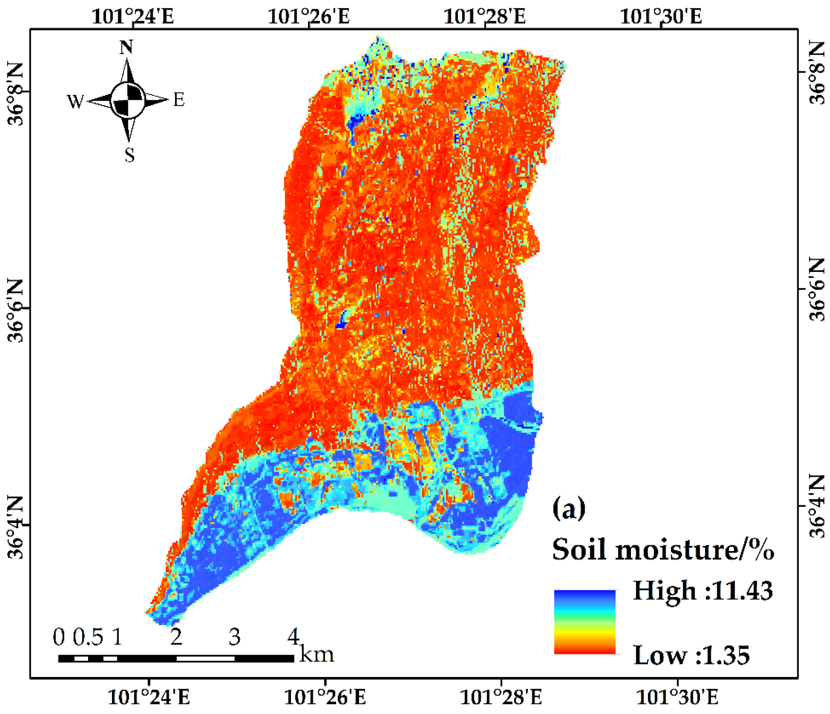
4.5. Spatial Distribution of Soil Moisture
5. Discussion
6. Conclusions
- (1)
- The importance of variables such as SR, VI, and TF is greater than SI and GP in inverting soil moisture in the Xiazangtan landslide area. The importance of variables such as SI and GP is greater than that of SR, VI, and TF in the soil moisture inversion model in the Xijitan landslide area. In addition, surface temperatures are more important in the Xijitan landslide area than in the Xiazangtan landslide area.
- (2)
- The accuracy of the soil moisture prediction model in the Xijitan landslide distribution area was 36.833% higher in R2 and 16.953% lower in RMSE in the model test set after screening the optimal independent variable combinations compared with that of the unscreened variables. The accuracy of the soil moisture prediction model for the Xiazangtan landslide distribution area increased by 15.456%, and the RMSE decreased by 5.614% for the model test set after screening with the optimal combination of independent variables compared to the unscreened variables.
- (3)
- The combined model showed the best relative applicability among the four soil moisture inversion models. The test set R2 of the integrated model was 0.916, and the RMSE was 0.877%. In addition, the overall accuracy of the BPNN model is also higher than the other two individual models. It had the highest R2 of 0.809% and an RMSE of 0.875% with the test dataset.
Author Contributions
Funding
Institutional Review Board Statement
Informed Consent Statement
Data Availability Statement
Conflicts of Interest
References
- Seneviratne, S.I.; Corti, T.; Davin, E.L.; Hirschi, M.; Jaeger, E.B.; Lehner, I.; Orlowsky, B.; Teuling, A.J. Investigating Soil Moisture–Climate Interactions in a Changing Climate: A Review. Earth-Sci. Rev. 2010, 99, 125–161. [Google Scholar] [CrossRef]
- Vereecken, H.; Huisman, J.A.; Pachepsky, Y.; Montzka, C.; van der Kruk, J.; Bogena, H.; Weihermüller, L.; Herbst, M.; Martinez, G.; Vanderborght, J. On the Spatio-Temporal Dynamics of Soil Moisture at the Field Scale. J. Hydrol. 2014, 516, 76–96. [Google Scholar] [CrossRef]
- Lei, L.; Zheng, J.; Li, S.; Yang, L.; Wang, W.; Zhang, F.; Zhang, B. Soil Hydrological Properties’ Response to Long-Term Grazing on a Desert Steppe in Inner Mongolia. Sustainability 2023, 15, 16256. [Google Scholar] [CrossRef]
- Zhang, Z.Y. Rapid Measurement Method of Hydraulic Conductivity of Unsaturated Soil and Mechanism of Landslide Induced by Rainfall Infiltration; Beijing Jiaotong University: Beijing, China, 2023. [Google Scholar]
- Lagasio, M.; Pulvirenti, L.; Parodi, A.; Boni, G.; Rommen, B. Effect of the Ingestion in the WRF Model of Different Sentinel-Derived and GNSS-Derived Products: Analysis of the Forecasts of a High Impact Weather Event. Eur. J. Remote Sens. 2019, 52, 16–33. [Google Scholar] [CrossRef]
- Mirus, B.B. HydroMet: A New Code for Automated Objective Optimization of Hydrometeorological Thresholds for Landslide Initiation. Water 2021, 13, 1752. [Google Scholar] [CrossRef]
- Bronstert, A.; Creutzfeldt, B.; Graeff, T.; Hajnsek, I.; Heistermann, M.; Itzerott, S.; Jagdhuber, T.; Kneis, D.; Lück, E.; Reusser, D.; et al. Potentials and Constraints of Different Types of Soil Moisture Observations for Flood Simulations in Headwater Catchments. Nat. Hazard. 2012, 60, 879–914. [Google Scholar] [CrossRef]
- Yin, Z.Q.; Cheng, G.M.; Hu, G.S.; Wei, G.; Wang, Y.Q. Prelm inary study on character istic and mechanism of super large landslide in upper Yellow River since late-pleistocene. J. Eng. Geol. 2010, 8, 41–51. [Google Scholar]
- Wang, S.; Li, R.; Wu, Y.; Wang, W. Estimation of Surface Soil Moisture by Combining a Structural Equation Model and an Artificial Neural Network (SEM-ANN). Sci. Total Environ. 2023, 876, 162558. [Google Scholar] [CrossRef] [PubMed]
- Babaeian, E.; Sadeghi, M.; Jones, B.S. Ground, Proximal, and Satellite Remote Sensing of Soil Moisture. Rev. Geophys. 2019, 57, 530–616. [Google Scholar] [CrossRef]
- Peng, J.; Albergel, C.; Balenzano, A.; Brocca, L.; Cartus, O.; Cosh, M.H.; Crow, W.T.; Dabrowska-Zielinska, K.; Dadson, S.; Davidson, M.W.J.; et al. A Roadmap for High-Resolution Satellite Soil Moisture Applications—Confronting Product Characteristics with User Requirements. Remote Sens. Environ. 2021, 252, 112162. [Google Scholar] [CrossRef]
- Gruber, A.; De Lannoy, G.; Albergel, C.; Al-Yaari, A.; Brocca, L.; Calvet, J.-C.; Colliander, A.; Cosh, M.; Crow, W.; Dorigo, W.; et al. Validation Practices for Satellite Soil Moisture Retrievals: What Are (the) Errors? Remote Sens. Environ. 2020, 244, 111806. [Google Scholar] [CrossRef]
- Pulvirenti, L.; Pierdicca, N.; Teuling, A.J. On the Potential of Sentinel-1 for Sub-Field Scale Soil Moisture Monitoring. Int. J. Appl. Earth Obs. Geoinf. 2023, 120, 103342. [Google Scholar]
- Yinglan, A.; Guoqiang, W.; Peng, H.; Xiaoying, L.; Baolin, X.; Qingqing, F. Root-Zone Soil Moisture Estimation Based on Remote Sensing Data and Deep Learning. Environ. Res. 2022, 212, 113278. [Google Scholar]
- Virnodkar, S.S.; Pachghare, V.K.; Patil, V.C.; Jha, S.K. Remote Sensing and Machine Learning for Crop Water Stress Determination in Various Crops: A Critical Review. Precis. Agric. 2020, 21, 1121–1155. [Google Scholar] [CrossRef]
- García-Tejero, I.F.; Rubio, A.E.; Viñuela, I.; Hernández, A.; Gutiérrez-Gordillo, S.; Rodríguez-Pleguezuelo, C.R.; Durán-Zuazo, V.H. Thermal Imaging at Plant Level to Assess the Crop-Water Status in Almond Trees (Cv. Guara) under Deficit Irrigation Strategies. Agric. Water Manag. 2018, 208, 176–186. [Google Scholar] [CrossRef]
- María, A.; Claudia, N.; Ángel, C.-B.M.; Miguel, A.L.; Jesús, Á.-M. Evaluation of Soil Moisture Estimation Techniques Based on Sentinel-1 Observations over Wheat Fields. Agric. Water Manag. 2023, 287, 108422. [Google Scholar]
- Zhang, Z.; Bian, J.; Han, W.; Fu, Q.P.; Chen, S.B.; Cui, T. Cotton moisture stress diagnosis based on canopy temperature characteristics calculated from UAV thermal infrared image. Trans. Chin. Soc. Agric. Eng. 2018, 34, 77–84. [Google Scholar] [CrossRef]
- Yu, Z.; Wenting, H.; Huihui, Z.; Xiaotao, N.; Guomin, S. Evaluating Soil Moisture Content under Maize Coverage Using UAV Multimodal Data by Machine Learning Algorithms. J. Hydrol. 2023, 617, 129086. [Google Scholar]
- Hong, Q.; Sun, H.; Chen, Y.S. Comparisons and Classification System of Typical Remote Sensing Indexes for Agricultural Drought. Trans. Chin. Soc. Agric. Eng. 2012, 28, 147–154. [Google Scholar]
- Guide County Local Records Compilation Committee. Guide Yearbook (2021); Sanqin Press: Xi’an, China, 2021; Volume 12. [Google Scholar]
- Hua, Q.C. Changes of Live—top Biomass, Plant Diversity and Soil Factors at Sunny and Shady Slope on Alpine Kobresia Meadow. J. Grassl. Forage Sci. 2024, 4, 22–25. [Google Scholar]
- Lu, S.L.; Liu, S.W.; Wu, Z.L.; Ho, T.N.; Zhou, L.H.; Huang, R.F.; Pan, J.T.; Editorial Committee of Flora of China, Chinese Academy of Sciences. Flora of China; Science Press: Beijing, China, 1993; Volume 4, pp. 156–161. [Google Scholar]
- Tucker, C.J. Red and Photographic Infrared Linear Combinations for Monitoring Vegetation. Remote Sens. Environ. 1979, 8, 127–150. [Google Scholar] [CrossRef]
- Yi, Q.X. Remote estimation of cotton LAI using Sentinel-2 multispectral data. Trans. Chin. Soc. Agric. Eng. 2019, 35, 189–197. [Google Scholar]
- Yuxiang, Z.; Jiheng, H.; Dasa, G.; Haixu, B.; Yuyun, F.; Yipu, W.; Rui, L. Simulation of Isoprene Emission with Satellite Microwave Emissivity Difference Vegetation Index as Water Stress Factor in Southeastern China during 2008. Remote. Sens. 2022, 14, 1740. [Google Scholar]
- Zhijun, Z.; Shengbo, C.; Tiangang, Y.; Eric, C.; Nicolas, L.; Jordan, G.; Michael, H.; Wenhan, Q.; Lisai, C.; Jian, L.; et al. Using the Negative Soil Adjustment Factor of Soil Adjusted Vegetation Index (SAVI) to Resist Saturation Effects and Estimate Leaf Area Index (LAI) in Dense Vegetation Areas. Sensors 2021, 21, 2115. [Google Scholar] [CrossRef] [PubMed]
- Qin, J.; Ma, M.; Shi, J.; Ma, S.; Wu, B.; Su, X.; Su, X. The Time-Lag Effect of Climate Factors on the Forest Enhanced Vegetation Index for Subtropical Humid Areas in China. Int. J. Environ. Res. Public Health 2023, 20, 799. [Google Scholar] [CrossRef] [PubMed]
- Allbed, A.; Kumar, L.; Aldakheel, Y.Y. Assessing Soil Salinity Using Soil Salinity and Vegetation Indices Derived from IKONOS High-Spatial Resolution Imageries: Applications in a Date Palm Dominated Region. Geoderma 2014, 231, 1–8. [Google Scholar] [CrossRef]
- Liu, H.Q.; Huete, A. A Feedback Based Modification of the NDVI to Minimize Canopy Background and Atmospheric Noise. IEEE Trans. Geosci. Remote Sens. 1995, 33, 457–465. [Google Scholar] [CrossRef]
- Khan, N.M.; Rastoskuev, V.V.; Sato, Y.; Shiozawa, S. Assessment of Hydrosaline Land Degradation by Using a Simple Approach of Remote Sensing Indicators. Agric. Water Manag. 2005, 77, 96–109. [Google Scholar] [CrossRef]
- Liu, H.J.; Wang, X.; Zhang, X.K.; Zhang, X.L.; Jin, H.N.; Dou, X. High spectral prediction model for soil moisture in songnen plain. Chin. J. Soil Sci. 2018, 49, 38–44. [Google Scholar]
- Sobrino, J.A.; Jiménez-Muñoz, J.C.; Soria, G.; Romaguera, M.; Guanter, L.; Moreno, J.F.; Plaza, A.J.; Martínez, P. Land Surface Emissivity Retrieval from Different VNIR and TIR Sensors. IEEE Trans Geosci. Remote Sens. 2008, 46, 316–327. [Google Scholar] [CrossRef]
- Yang, L.P.; Ren, J.; Wang, Y.; Zhang, J.; Wang, T.; Li, K. Soil Salinity Estimation Model in Juyanze Based on Multi-source Remote Sensing Data. Tran. Chin. Soc. Agric. Mach. 2022, 53, 226–235. [Google Scholar]
- Krzeminska, D.; Bloem, E.; Starkloff, T.; Stolte, J. Combining FDR and ERT for monitoring soil moisture and temperature patterns in undulating terrain in south-eastern Norway. Catena 2022, 212, 106100. [Google Scholar] [CrossRef]
- Wang, S.N.; Li, R.P.; Wu, Y.J.; Zhao, S.X.; Wang, X.Q. Multi-model comprehensive inversion of surface soil moisture based on model averaging method. Trans. Chin. Soc. Agric. Eng. 2022, 38, 87–94. [Google Scholar]
- Sohrabinia, M.; Rack, W.; Zawar-Reza, P. Errata: Soil Moisture Derived Using Two Apparent Thermal Inertia Functions over Canterbury, New Zealand. Remote Sens. 2014, 8, 083624. [Google Scholar] [CrossRef]


| Variable Group | Variable Name | Formulas and Notes |
|---|---|---|
| BR | B2, B3, B4, B5, B6, B7 | Reflectance in , , , , , and bands. |
| VI | NDVI [24] | |
| RVI [25] | ||
| DVI [26] | ||
| SAVI [27] | ||
| EVI [28] | ||
| GVI [28] | ||
| SI | SI-T [29] | |
| S1 [30] | ||
| S2 [30] | ||
| S3 [30] | ||
| NDSI [31] | ||
| GP | Bright [32] | |
| Green [32] | ||
| Wet [32] | ||
| Albedo [21] | ||
| NDWI [21] | ||
| NDBI [21] | ||
| TF | Elevation, AS, S | Elevation, Slope direction, Gradient |
| Combination Criteria | Combined Serial Number | Variable Combinations | Preferred Environment Variables | |
|---|---|---|---|---|
| Xijitan | Xiazangtan | |||
| All variable | 1 | BR + VI | B2, B3, B4, B5, B6, B7, NDVI, RVI, DVI, SAVI, EVI, GVI, DBWD | |
| 2 | BR + VI + SI | B2, B3, B4, B5, B6, B7, NDVI, RVI, DVI, SAVI, EVI, GVI, SI-T, S1, S2, S3, NDSI, DBWD | ||
| 3 | BR + VI + SI + GP | B2, B3, B4, B5, B6, B7, NDVI, RVI, DVI, SAVI, EVI, GVI, SI-T, S1, S2, S3, NDSI, Bright, Green, Wet, Albedo, MDWI, NDBI, DBWD | ||
| 4 | BR + VI + SI + GP + TF | B2, B3, B4, B5, B6, B7, NDVI, RVI, DVI, SAVI, EVI, GVI, SI-T, S1, S2, S3, NDSI, Bright, Green, Wet, Albedo, MDWI, NDBI, S, AS, ELEVATION, DBWD | ||
| Top 1 in importance | 5 | BR + VI | B5, GVI, DBWD | B2, NDVI, DBWD |
| 6 | BR + VI + SI | B5, GVI, S1DBWD | B2, NDVI, NDSI, DBWD | |
| 7 | BR + VI +SI + GP | B5, GVI, S1, NDBI, DBWD | B2, NDVI, NDSI, WET, DBWD | |
| 8 | BR + VI + SI + GP + TF | B5, GVI, S1, NDBI, E, DBWD | B2, NDVI, NDSI, WET, E, DBWD | |
| Top 2 in importance | 9 | BR + VI | B5, B3, GVI, RVI, DBWD | B2, B7, NDVI, RVI, DBWD |
| 10 | BR + VI + SI | B5, B3, GVI, RVI, S1, S2, DBWD | B2, B7, NDVI, RVI, NDSI, SI-T, DBWD | |
| 11 | BR + VI + SI + GP | B5, B3, GVIRVI, S1, S2, NDBI, MDWI, DBWD | B2, B7, NDVI, RVI, NDSI, SI-T, WET, NDBI, DBWD | |
| 12 | BR + VI + SI + GP + TF | B5, B3, GVI, RVI, S1, S2, NDBI, MDWI, E, S, DBWD | B2, B7, NDVI, RVI, NDSI, SI-T, WET, NDBI, E, AS, DBWD | |
| Top 3 in importance | 13 | BR + VI | B5, B3, B4, GVI, RVI, NDVI, DBWD | B2, B7, B3, NDVI, RVI, GVI, DBWD |
| 14 | BR + VI + SI | B5, B3, B4, GVI, RVI, NDVI, S1, S2, SI-T, DBWD | b2, b7, b3, NDVI, RVI, GVI, NDSI, SI-T, S3, DBWD | |
| 15 | BR + VI + SI + GP | B5, B3, B4, GVI, RVI, NDVI, S1, S2, SI-T, NDBI, MDWI, Albedo, DBWD | B2, B7, B3, NDVI, RVI, GVI, NDSI, SI-T, S3, Wet, NDBI, Albedo, DBWD | |
| 16 | BR + VI + SI + GP + TF | B5, B3, B4, GVI, RVI, NDVI, S1, S2, SI-T, NDBI, MDWI, Albedo, E, S, AS, DBWD | B2, B7, B3, NDVI, RVI, GVI, NDSI, SI-T, S3, Wet, NDBI, Albedo, E, AS, S, DBWD | |
| Top 4 in importance | 17 | BR + VI | B5, B3, B4, B2, GVI, RVI, NDVI, EVI, DBWD | B2, B7, B3, B4, NDVI, RVI, GVI, DVI, DBWD |
| 18 | BR + VI + SI | B5, B3, B4, B2, GVI, RVI, NDVI, EVI, S1, S2, SI-T, NDSI, DBWD | B2, B7, B3, B4, NDVI, RVI, GVI, DVI, NDSI, SI-T, S3, S1, DBWD | |
| 19 | BR + VI + SI + GP | B5, B3, B4, B2, GVI, RVI, NDVI, EVI, S1, S2, SI-T, NDSI, NDBI, MDWI, Albedo, Green, DBWD | B2, B7, B3, B4, NDVI, RVI, GVI, DVI, NDSI, SI-T, S3, S1, WET, NDBI, Albedo, MDWI, DBWD | |
| 20 | BR+VI+SI+GP+TF | B5, B3, B4, B2, GVI, RVI, NDVI, EVI, S1, S2, SI-T, NDSI, NDBI, MDWI, Albedo, Green, E, S, AS, DBWD | B2, B7, B3, B4, NDVI, RVI, GVI, DVI, NDSI, SI-T, S3, S1, WET, NDBI, Albedo, MDWI, E, AS, S, DBWD | |
| Modelling Methodology | Train | Test | ||||||
|---|---|---|---|---|---|---|---|---|
| R2 | RMSE | MAE | MBE | R2 | RMSE | MAE | MBE | |
| RF | 0.656 | 1.862 | 0.880 | −0.011 | 0.562 | 2.100 | 1.142 | 0.021 |
| SVM | 0.956 | 0.655 | 0.353 | −0.071 | 0.833 | 1.375 | 0.980 | −0.075 |
| BPNN | 0.922 | 0.952 | 0.651 | −0.082 | 0.809 | 0.875 | 0.695 | −0.228 |
| Combined model | 0.886 | 1.085 | 0.690 | −0.001 | 0.916 | 0.877 | 0.620 | 0.154 |
Disclaimer/Publisher’s Note: The statements, opinions and data contained in all publications are solely those of the individual author(s) and contributor(s) and not of MDPI and/or the editor(s). MDPI and/or the editor(s) disclaim responsibility for any injury to people or property resulting from any ideas, methods, instructions or products referred to in the content. |
© 2024 by the authors. Licensee MDPI, Basel, Switzerland. This article is an open access article distributed under the terms and conditions of the Creative Commons Attribution (CC BY) license (https://creativecommons.org/licenses/by/4.0/).
Share and Cite
Lv, W.; Hu, X.; Li, X.; Zhao, J.; Liu, C.; Li, S.; Li, G.; Zhu, H. Multi-Model Comprehensive Inversion of Surface Soil Moisture from Landsat Images Based on Machine Learning Algorithms. Sustainability 2024, 16, 3509. https://doi.org/10.3390/su16093509
Lv W, Hu X, Li X, Zhao J, Liu C, Li S, Li G, Zhu H. Multi-Model Comprehensive Inversion of Surface Soil Moisture from Landsat Images Based on Machine Learning Algorithms. Sustainability. 2024; 16(9):3509. https://doi.org/10.3390/su16093509
Chicago/Turabian StyleLv, Weitao, Xiasong Hu, Xilai Li, Jimei Zhao, Changyi Liu, Shuaifei Li, Guorong Li, and Haili Zhu. 2024. "Multi-Model Comprehensive Inversion of Surface Soil Moisture from Landsat Images Based on Machine Learning Algorithms" Sustainability 16, no. 9: 3509. https://doi.org/10.3390/su16093509