Green Fiscal and Tax Policies in China: An Environmental Dynamic Stochastic General Equilibrium Approach

Abstract

Implementing green fiscal and tax policies for reducing emissions and pollution without negatively impacting economic growth remains a challenge. We aimed to determine whether environmental protection and economic growth can both be attained under a green fiscal and tax policy. Specifically, we created a dynamic stochastic general equilibrium (DSGE) model to explore the environmental, economic, and welfare impacts of green fiscal and tax policies. Additionally, a welfare analysis based on an environmental DSGE (E-DSGE) model was performed. We found that (1) raising the environmental or energy tax rate was beneficial for reducing emissions and environmental pollution. However, this approach inhibited economic growth, an outcome not conducive to improving welfare. (2) Increasing the subsidy rate for emission reduction not only incentivized businesses to reduce emissions but also improved economic growth and welfare. (3) The emission reduction mechanisms of environmental tax policies, energy tax policies, and subsidy policies are different. Among them, the environmental tax policy and the energy tax policy both reduce pollution by forcing businesses to increase their emission reduction efforts, but the former is a tax on pollution emissions, while the latter is a tax on energy consumption. However, emission reduction subsidy policies incentivize companies to increase their emission reduction efforts and reduce pollution emissions by alleviating their financial burden. (4) Increasing government spending on environmental remediation could promote economic growth. However, considering that this does not motivate companies to reduce emissions, increasing their share will lead to a reduction in emission reduction subsidies, ultimately negatively impacting social welfare. (5) An environmental tax would cause greater losses in welfare than an energy tax. These findings will enable policymakers to optimize expenditures and tax systems.

1. Introduction

To promote ecological environmental governance and address climate change, China has emphasized the importance of achieving a balance between economic growth and the maintenance of ecological integrity. Fiscal and tax policies are indispensable for encouraging or forcing businesses to reduce emissions, thus improving the quality of the ecological environment, promoting green and low-carbon transformations, and addressing climate change. The Chinese government is in the process of implementing various green fiscal and tax policies, including environmental taxes, resource taxes, tax incentives, energy conservation policies, emission reduction subsidies, and government spending on pollution treatments. These policies have all had a significant impact by encouraging or forcing businesses to reduce their emissions by improving production techniques and management models, controlling pollutant emissions, and improving the quality of their environment. However, there are significant differences among the impacts of different green fiscal and tax policies on the real economy, which can not only improve business production and promote real-economy development but can also increase the burden on businesses, which is not conducive to economic development. In particular, during an economic downturn, the adoption of certain green fiscal and tax policies may impede the development of the real economy, resulting in a decline in social welfare. Since entering the New Normal, China’s economic development has entered a “three-phase superposition” stage: namely, periods with a shifting growth speed, painful structural adjustment, and the digestion of early stimulus policies, which have resulted in certain downward pressure on economic operation. Following the outbreak of the COVID-19 pandemic, the external and internal environments confronting China’s economic growth have become more complicated, severe, and uncertain, placing further downward pressure on the economy.

Thus, ensuring the effective implementation of green fiscal and tax policies for reducing emissions and pollution while avoiding adverse impacts on the real economy is a major challenge faced by policy departments. Additionally, whether in the form of ecological or economic benefits, the ultimate goal of green fiscal and tax policies is to improve social welfare and meet people’s requirements for improving their quality of life. Therefore, conducting in-depth research on the macroeconomic, environmental, and welfare effects of various green fiscal and tax policies, as well as seeking triple-win policies that balance environmental protection, economic growth, and social welfare or tax policies that have less of an impact on economic growth and social welfare, is of great significance for reducing the adverse effects of green fiscal and tax policies. Moreover, China is currently promoting the construction of a green fiscal and tax system in order to better leverage the fundamental role of fiscal and tax policies, which, naturally, calls for more comprehensive and in-depth research into the impacts of green fiscal and tax policies.

2. Literature Review

Various methods have been used to elucidate the economic impact of environmental policies, including static general equilibrium analysis [1], endogenous growth models [2,3,4], computable general equilibrium (CGE) models [5,6,7,8,9], game models [10], and econometric models [11,12]. However, in the context of this issue, there is still significant controversy, which can be seen from three main viewpoints. The first is that environmental policies can inhibit social investment, negatively impacting economic growth [2,5,9,12,13,14]. For example, Bovenberg and Smulders [2] investigated the economic effects of emission tax policies within the framework of the Ramsey model and found that imposing a pollution tax had a crowding-out effect on private investment, thereby suppressing economic growth. Aydin [5] and Withey et al. [8] studied the economic impact of carbon taxes based on a computable general equilibrium (CGE) model and reached similar conclusions. On the other hand, Gu et al. [9] focused on studying the economic impact of carbon tariffs and found that carbon tariffs negatively impacted economic growth, resident welfare, and internal trade within the subject country. Si et al. [12] conducted an empirical study on the economic impact of environmental policies, and their conclusions also support this viewpoint. The second viewpoint suggests that appropriate environmental policies can not only reduce pollution emissions but also positively impact economic growth [1,4,10,15,16]. For example, Orlov et al. [1] revealed that replacing labor taxes with carbon taxes not only reduced carbon emissions but also enhanced social welfare. Ikefuji and Ono [4] explored environmental policies under unemployment and found that imposing emission taxes can stimulate employment and consumption, thereby promoting economic growth. Constantatos et al. [10] further found that regardless of whether taxation is aimed at output or emissions, the levels of economic output and pollution emissions are better than those without taxation, resulting in greater social welfare. He et al. [11] conducted an empirical test using the panel autoregressive distribution lag (ARDL) model and found that in the long run, environmental taxes had a dual dividend effect. The third viewpoint is that whether environmental tax policies harm or promote economic growth depends on whether their growth path is determined. Itaya [3] found that when the equilibrium growth path was uncertain, environmental taxes usually promoted long-term growth. In contrast, when the equilibrium growth path was determined, environmental taxes impeded long-term growth.

Recently, a macroeconomic model, the DSGE, has been used to evaluate the environmental and economic effects of conventional environmental regulation policies, green fiscal policies, and green finance policies. In terms of traditional environmental regulation policies, researchers have largely focused on the environmental and economic impacts of policies such as environmental taxes, emission intensity, emission quotas, emission targets, and emission rules or compared and analyzed their policy effects. Furthermore, Fischer and Springborn [17] researched the impact of environmental policies on economic growth and volatility. The results showed that the intensity target policy maintained higher levels of labor, capital, and output than those of policies such as carbon taxes, emission quotas, or emission targets, while also having lower expected costs and no greater volatility than without policies. Additionally, Xiao et al. [18] studied the influence of environmental taxes, emission intensity plans, and emission permits on the business cycle and found that emission intensity plans showed the greatest inhibitory effect on economic fluctuations. Meanwhile, Angelopoulos et al. [19] compared the effects of environmental policies such as carbon taxes, emission permits, and carbon emission rules on overall social welfare, revealing that emission permits were the worst option, while carbon taxes outperformed emission rules. Heutel [20] investigated the issue of optimal emission reduction policies and revealed that these policies suppressed the procyclicality of emissions. In addition, Annicchiarico and Dio [21] investigated the macroeconomic dynamics underlying various environmental policies using the New Keynesian DSGE model, revealing that staggered price adjustments and monetary policy responses significantly altered the effectiveness of environmental policies. Wang et al. [22] explored the win–win problem presented by environmental policies, suggesting that these policies would invariably result in lower output levels, rendering it difficult to balance environmental governance and economic development.

In terms of green fiscal policies, the primary emphasis is still placed on examining the economic and environmental impacts of overall environmental spending, emission reduction subsidies, and pollution prevention and control expenditures. Pan et al. [23] previously examined the spatial effects of local government environmental expenditures and found that local government environmental expenditures displaced local consumption and investment but had a positive impact on the economic growth of other regions. Meanwhile, Wu [24] discovered that the effects of emissions reduction subsidies on economic growth manifested as short-term promotion and long-term inhibition, whereas the opposite was true for impacts on environmental quality. Striking a balance between environmental governance and economic growth is challenging. However, Cai et al. [25] reached a different conclusion, stating that carbon emission subsidies could help to promote economic growth but were not conducive to improving environmental quality.

Most previous studies on the effects of green finance policies on the economy and environment have been conducted by constructing models of heterogeneous production sectors. Punzi [26] evaluated the effects of technological, monetary, and credit shocks on the green production sector and reported that only favorable credit shocks could foster long-term growth. Scholars have primarily conducted research focused on the environmental and economic impacts of green finance policies by constructing heterogeneous production sector models. According to Wang et al. [27], applying a particular level of credit incentives to green production companies can optimize the structure of the economy, leading to a win–win scenario for both “economic growth” and “environmental protection”. In a further study by Liu and He [28], the output and welfare effects of green credit policies were examined in relation to environmental regulations. These findings indicated that the economic effects of green credit policies were slightly muted in the presence of environmental taxes.

There has been extensive research into the economic effects of environmental policies, although the majority of these studies have focused on traditional environmental regulation policies and green finance policies, with less research conducted on green fiscal policies. Although some studies have used the DSGE model to analyze the economic and environmental consequences of green fiscal policies [23,24,25], they have been primarily focused on the spatial implications of policies and their impact on environmental quality. Additionally, considering that most of these studies include businesses’ emission reduction efforts as exogenous factors, it is difficult to gain insights into the internal processes of policies working on economic and environmental variables, and there have been no strong conclusions obtained regarding this. Thus, we considered whether environmental protection and economic growth can coexist peacefully under a green fiscal and tax policy. It is also unclear as to how we can select green fiscal strategies to prevent negative effects on economic growth and social welfare when facing the simultaneous pressures of environmental pollution and the growth of the real economy. To investigate these two concerns, this study built a DSGE model incorporating four primary green fiscal policies: environmental taxes, energy taxes, emission reduction subsidies, and government spending on pollution treatments. In China’s fiscal expenditure structure, environmental expenditure mainly includes energy conservation and emission reduction expenditures, as well as pollution prevention and control expenditures. In China’s tax system structure, in addition to environmental taxes, other environmentally friendly taxes include the energy tax, consumption tax, and urban land use tax, with energy taxes playing the most important role besides environmental taxes. Therefore, this article selected the four types of green fiscal and tax policies mentioned above.

The aim of this study was to determine whether environmental protection and economic growth could coexist under a green fiscal and tax policy. Overall, the contributions of this study are threefold. (1) It extends the theoretical framework of environmental economics by incorporating environmental pollution and green fiscal policies into a dynamic stochastic general equilibrium (DSGE) model. (2) It also combines four key green fiscal and tax policy instruments in one analytical framework, enabling the examination of the implication of green fiscal and tax policies on macroeconomics, ecological integrity, and welfare. (3) Compared to previous research on green finance and taxation, the way in which this study sets a business’ abatement effort as an endogenous variable allows for a more robust characterization of the mechanisms underlying green fiscal and tax policies that affect macroeconomic and environmental variables by influencing corporate behavior.

3. The Model

The economic system is described using a simple New Keynesian model with nominal price rigidities and financing constraints, including pollutant emissions (pollutant emissions and carbon emissions are highly homologous, and this article does not distinguish between environmental pollutants and carbon emissions but collectively refers to them as environmental pollutants), green fiscal and tax policies, and a negative externality of pollution on labor efficiency. This system also accurately characterizes competitive intermediate goods producers using capital, labor, and energy to produce intermediate goods and emit pollutants; monopolistically competitive retailers purchase intermediate goods and repackage and label them before reselling them to the final goods producers; perfectly competitive final goods producers combine differentiated intermediate goods to produce final consumption goods; and households that consume and supply production factors. The government is the implementer of green fiscal and tax policies; it collects revenue by taxing and borrowing and then using this for various expenditures (see Figure 1). Assuming that there is no friction in the financial market and that the household sector’s deposits flow freely to businesses and the government, we omitted the modeling of financial intermediaries.

3.1. Production

3.1.1. Final Goods Producers

The final product $Y_t$ is produced by perfectly competitive final goods producers using the differentiated intermediate products via the Cobb–Douglas production function [29]: $Y_t={\left({\int }_0^1{y_{f,t}}^{(\theta -1)/\theta }df\right)}^{(\theta /(\theta -1))}$, with $\theta >1$ being the alternative elasticity of differentiated intermediate products, whilst $y_{f,t}$ represents the differentiated intermediate goods. The equation for maximizing profits for the final goods producers is as follows: $\underset{y_{f,t}}{\max }{P}_t{Y}_t-{\int }_0^1{P}_{f,t}{y}_{f,t}df$. By optimizing the equations above, we obtain the final product’s business demand function for the differentiated intermediate products, $y_{f,t}={\left(P_{f,t}/P_t\right)}^{-\theta }{Y}_t$, where $P_t={\left({\int }_0^1{P_{f,t}}^{1-\theta }df\right)}^{1/(1-\theta )}$. There is a continuum $f\in [\mathrm{0,1}]$ of monopolistically competitive final goods producers.

3.1.2. Retail

Monopolistically, competitive retailers have pricing power over differentiated intermediate goods. A retailer $f$ purchases an undifferentiated intermediate product $y_{i,t}$ from intermediate goods producers at a relative price ${mc}_t$ and converts it into differentiated intermediate products $y_{f,t}$ in a 1:1 ratio. Assuming that retailers follow Calvo’s pricing rule [30], those with a $\xi$ ratio can adjust their prices based on prices from the previous period, whereas those with other $1-\xi$ ratios can make adjustments based on prices from the previous period. The optimization problem for the intermediate retailers is as follows:

$$\underset{P_{f,t}}{\max } {\mathrm{E}}_t{\sum }_{j=0}^{\infty }{({\beta }_h\xi )}^i{\lambda }_{t+i}^h\left(\frac{P_{f,t}-P_{t+i}{mc}_{t+i}}{P_{t+i}}\right)y_{f,t+i}$$

(1)

By solving the above optimization equation, we can obtain the optimal pricing conditions for intermediate retailers.

$$p_{f,t}^{*}=\frac{\theta }{\theta -1}\frac{{\mathrm{E}}_t{\sum }_{i=0}^{\infty }{\left({\beta }_h\xi \right)}^i{\lambda }_{t+i}{mc}_{t+s}{\left(\frac{P_{t+s}}{P_t}\right)}^{\theta }{Y}_{t+i}}{{\mathrm{E}}_t{\sum }_{i=0}^{\infty }{\left({\beta }_h\xi \right)}^i{\lambda }_{t+i}{\left(\frac{P_{t+i}}{P_t}\right)}^{\theta -1}{Y}_{t+i}}$$

(2)

3.1.3. Intermediate Goods Producers

Perfectly competitive intermediate goods producers use capital $K_t$, labor $L_t$, and energy $M_t$ to produce undifferentiated intermediate goods using the necessary Cobb–Douglas technology [18].

$$y_t=A_t{\left(K_{t-1}\right)}^{{\alpha }_1}{\left(e_t^L{L}_t\right)}^{{\alpha }_2}{\left(M_t\right)}^{1-{\alpha }_1-{\alpha }_2}$$

(3)

where $A_t$ is the total factor productivity and an exogenous process is followed; $ln{A}_t=\left(1-{\rho }_A\right)ln\overline{A}+{\rho }_{A}ln{A}_{t-1}+{\epsilon }_{A,t}$, where $\overline{A}$ is the mean value or steady state value of $A_t$; and ${\epsilon }_{A,t}$ is white noise. In addition, ${\alpha }_1$ is the elasticity of output with respect to capital, while ${\alpha }_2$ is the elasticity of output with respect to labor. The capital stock evolves at a decay rate ${\delta }_K$: $K_t=\left(1-{\delta }_K\right)K_{t-1}+X_t$, where $X_t$ represents the net investment [22]. The externality of environmental pollution is reflected in the damage that it causes to the health of workers [31,32], leading to the loss of labor efficiency [33]. With reference to Xiao et al. [18] and Pan et al. [23], we set the labor efficiency $e_t^L$ as a decreasing concave function of the pollution stock ${PS}_t$.

$$e_t^L=1-d_0-d_1\times {PS}_t-d_2\times {{PS}_t}^2$$

(4)

In Formula (4), $d\left(PS\right)=d_2\times {{PS}_t}^2+d_1\times PS+d_0$ represents the health loss function.

Excessive consumption of fossil fuels is the most important cause of environmental pollution. Due to China’s fossil energy consumption accounting for over 80% of energy consumption, it is assumed that pollutant emissions are a function of energy consumption: ${Em}_t={\phi M}_t$, where $\phi$ represents the pollutant emissions per unit of energy consumption [18]. In reality, the pollutant emissions of producers are also related to their abatement efforts $U_t$, as we assumed ${Ea}_t={(1-U_t)\phi M}_t$, and the emission intensity is ${Intensity}_t=\frac{{Ea}_t}{y_t}$.

Due to the negative externality of environmental pollution, the government levies an environmental tax on the pollutant discharge of intermediate goods producers. Assuming that the environmental tax rate set by the government is ${tau}_t^E$, the environmental tax that intermediate production businesses must pay is as follows:

$${tax}_t^E={tau}_t^E{(1-U_t)\phi M}_t$$

(5)

The emission reduction activities of intermediate production businesses reduce their pollutant emissions while increasing their production costs. We set the emission reduction costs for intermediate goods producers as a function of abatement efforts and energy consumption [21].

$${CA}_t={\varphi }_1{\left(U_t\right)}^{{\varphi }_2}{M}_t$$

(6)

where ${\varphi }_1$ and ${\varphi }_2$ represent the technical parameters for pollution reduction and ${\varphi }_1>0$, ${\varphi }_2>0$.

The government subsidizes the emission reduction behavior of intermediate goods producers. Assuming that the government’s emission reduction subsidy to intermediate goods producers is ${Gsub}_t$, which is positively correlated with the subsidy rate $s_t$ and abatement efforts $U_t$, while being negatively correlated with pollutant emissions ${Em}_t$, the emission reduction subsidy function can be expressed as follows:

$${Gsub}_t=\frac{s_t{U}_t}{{\phi M}_t}$$

(7)

Prior research demonstrates that financing constraints have a significant impact on the development of Chinese firms [34]. Consequently, this study adds the institutional aspect of financing constraints to the model to describe businesses’ traits and behaviors more accurately. Referring to Kiyotaki and Moore [35] and Iacoviello [36], we imposed financing constraints on intermediate goods producers. Assuming that intermediate goods producers obtain financing by mortgaging capital, the financing constraints faced by a business are given by Formula (8):

$$b_{e,t}\le m_b{E}_t\frac{q_{t+1}^K{K}_t{\pi }_{t+1}}{R_t}$$

(8)

where $b_{e,t}$ represents the maximum loan amount obtained by intermediate goods producers, ${\pi }_t$ is the inflation rate, and $\frac{q_{t+1}^K{K}_t{\pi }_{t+1}}{R_t}$ represents the actual value of the collateral. Furthermore, $m_b\le 1$ represents the degree of financing constraints; the higher the value, the more relaxed the financing conditions, and, conversely, the tighter the financing conditions. This formula reflects the restrictive effect of collateral value on corporate financing.

Entrepreneurs are owners of intermediate goods businesses who not only carry out financing activities for themselves but also earn all the income from intermediate products. Assuming that entrepreneurs obtain positive utility through consumption, their optimal decision is to maximize the present value of their future consumption utility in each period [22].

$$E_0{\sum }_{t=0}^{\infty }{\left({\beta }_e\right)}^{t}ln{C}_{e,t}$$

(9)

where $E_0$ represents the conditional expectation operator, $C_{e,t}$ represents entrepreneur consumption, and ${\beta }_e$ represents the subjective discount factor of entrepreneur consumption. Intermediate goods producers are subject to technology constraints and the flow of funds [36], as given by Equation (10).

$${mc}_t{y}_t+b_{e,t}=C_{e,t}+b_{e,t-1}\frac{R_{t-1}}{{\pi }_t}+w_t{L}_t+q_t^K{X}_t+p_t^M{M}_t+{\varphi }_1{\left(U_t\right)}^{{\varphi }_2}{M}_t+{tau}_t^E\left(1-U_t\right)\phi M_t-\frac{s_t{U}_t}{{\phi M}_t}$$

(10)

In Equation (10), ${mc}_t$ is the relative price of undifferentiated intermediate goods, $w_t$ is the labor wage rate, $q_t^K$ is the net investment price, and $p_t^M$ is the energy price.

By solving the problem of maximizing the utility of entrepreneurs, we can obtain the first-order conditions for $C_{e,t}$, $b_{e,t}$, $L_t$, $K_t$, $M_t$, and $U_t$.

$${\left(C_{e,t}\right)}^{-1}={\lambda }_{e,t}$$

(11)

$${\lambda }_{e,t}={\beta }_e{\lambda }_{e,t+1}\frac{R_t}{{\pi }_{t+1}}+{\lambda }_{b,t}$$

(12)

$$w_t={\alpha }_2{mc}_t\frac{y_t}{L_t}$$

(13)

$${\lambda }_{e,t}{q}_t^K={\beta }_e{\lambda }_{e,t+1}\left[{\alpha }_1{mc}_{t+1}\frac{y_{t+1}}{K_t}+q_{t+1}^K(1-{\delta }_K)\right]+{\lambda }_{b,t}{m}_b\frac{q_{t+1}^K{\pi }_{t+1}}{R_t}$$

(14)

$$p_t^M+{\left({\varphi }_1{U}_t\right)}^{{\varphi }_2}+{tax}_t^E(1-U_t)\phi +s_t\frac{U_t}{{\phi \left(M_t\right)}^2}=(1-{\alpha }_1-{\alpha }_2){mc}_t\frac{y_t}{M_t}$$

(15)

$${\varphi }_1{\varphi }_1{\left(U_t\right)}^{{\varphi }_2-1}{M}_t-{tau}_t^E\phi M_t=\frac{s_t}{{\phi M}_t}$$

(16)

3.2. Households

The household sector adopts the classic setting of the DSGE model, which assumes that there are countless homogeneous and infinitely viable households in the economy and also that households maximize their utility by optimizing the sum of their present utility values for each period. Households derive utility from consumption $C_t$ and disutility from labor $L_t$ and pollutant emissions ${Ea}_t$. The family objective function is expressed as follows [18]:

$$\underset{C_t,L_t,M_t,d_t,I_t}{\max } E_0{\sum }_{t=0}^{\infty }{\left(\beta \right)}^t\left\{ln{C}_t-{\mu }_L\frac{{\left(L_t\right)}^{1+\eta }}{1+\eta }-{\mu }_M\frac{{\left({Ea}_t\right)}^{1+\nu }}{1+\nu }\right\}$$

(17)

where $\beta$ represents the subjective discount factor of the family and $0<\beta <1$; $C_t$ represents the actual consumption of households; ${\mu }_L$ is the negative utility coefficient of labor, whilst $\eta$ is the reciprocal of the elasticity of the household labor supply; and ${\mu }_M$ is the negative utility coefficient of pollutant emissions, with $\nu$ being the elasticity of the energy supply. The household sector budget constraints can be expressed as follows [22]:

$$d_t+C_t+I_t=\frac{R_{t-1}{d}_{t-1}}{{\pi }_t}+\left(1-{tau}^L\right)w_t{L}_t+\left(1-{tau}^K\right)q_t^K{X}_t+\left(1-{tau}_t^M\right)p_t^M{M}_t+{\sum }_t+{TR}_t$$

(18)

where $I_t$ represents household investment; $d_t$ represents the actual household savings, and the savings interest rate is $R_t$; ${TR}_t$ is the government’s transfer payment to households; $q_t^K$ is the net investment price; and ${tau}^L$, ${tau}^K$, and ${tau}_t^M$ represent the payroll, investment income, and energy tax rates, respectively. The relationship between investment $I_t$ and net investment $X_t$ is $X_t=I_t-\frac{{\Psi }_I}{2}{\left(\frac{I_t}{I_{t-1}}-1\right)}^2{I}_t$, where $\frac{{\Psi }_I}{2}{\left(\frac{I_t}{I_{t-1}}-1\right)}^2{I}_t$ is the investment adjustment cost and ${\Psi }_I$ is the investment adjustment cost coefficient [22].

The following first-order optimization conditions can be attained under the budget constraint by resolving the maximization of household utility:

$${\left(C_t\right)}^{-1}={\lambda }_t$$

(19)

$${\mu }_L{\left(L_t\right)}^{\eta }={\lambda }_t\left(1-{tau}^L\right)w_t$$

(20)

$${\mu }_M{\left(\right(1-U_t\left)\phi M_t\right)}^{1+\nu }={\lambda }_t\left(1-{tau}_t^M\right)p_t^E$$

(21)

$$1=\beta E_t\frac{{\lambda }_{t+1}}{{\lambda }_t}\frac{R_t}{{\pi }_{t+1}}$$

(22)

$$\frac{1}{\left(1-{\tau }^K\right)q_t^K}=1-{\Psi }_I\left(\frac{I_t}{I_{t-1}}-1\right)\left(\frac{I_t}{I_{t-1}}\right)-\frac{{\Psi }_I}{2}{\left(\frac{I_t}{I_{t-1}}-1\right)}^2+\beta E_t\frac{{\lambda }_{t+1}}{{\lambda }_t}\frac{q_{t+1}^K}{q_t^K}{\Psi }_I\left(\frac{I_{t+1}}{I_t}-1\right){\left(\frac{I_{t+1}}{I_t}\right)}^2$$

(23)

3.3. Evolution Equation for Pollution Stock

Environmental pollutants can be directly increased by pollutant emissions; however, they can also be reduced via both natural deterioration and human-made remediation. ${PS}_t$ denotes the pollution stock at the end of the period $t$, while ${Ge}_t$ denotes government spending on pollution treatment. This provides the following accumulation equation [19]:

$${PS}_t=\left(1-{\delta }_{PS}\right){PS}_{t-1}+{Ea}_t-\chi {Ge}_t$$

(24)

where ${\delta }_{PS}$ measures the fraction of pollution that naturally decays in each time period and $0\le {\delta }_{PS\le 1}$, while $\chi$ represents the effectiveness coefficient of government spending on pollution treatment.

3.4. Government Sector

Through taxation and bond issuance, the government generates income for various expenses. Assuming that the government adheres to the principle of balanced budget revenues and expenditures, its budgetary restrictions can be represented as follows:

$${tau}^L{w}_t{L}_t+{tau}^K{q}_t^K{X}_t+{tau}_t^M{p}_t^M{M}_t+{tax}_t^E+b_{g,t}=G_t$$

(25)

$$G_t=b_{g,t-1}\frac{R_t}{{\pi }_t}+{TR}_t+{Gsub}_t+{Ge}_t$$

(26)

where Equation (25) represents the composition of government revenue, including labor tax ${tau}^L{w}_t{L}_t$, capital tax ${tau}^K{q}_t^K{X}_t$, energy tax ${tau}_t^M{p}_t^M{M}_t$, environmental tax ${tax}_t^E$, and debt $b_{g,t}$ and Equation (26) represents the composition of government expenditure, including emission reduction subsidies ${Gsub}_t$, government spending on pollution treatment ${Ge}_t$, household transfer payments ${TR}_t$, and debt interest expenses $b_{g,t-1}\frac{R_t}{{\pi }_t}$.

3.5. Market Equilibrium

The goods and lending markets must simultaneously reach equilibrium in order for the economic system to remain stable.

In equilibrium, the goods market requires that

$$Y_t=C_t+C_{e,t}+I_t+{CA}_t+{Ge}_t$$

(27)

Moreover, the lending market’s equilibrium satisfies

$$d_t=b_{e,t}+b_{g,t}$$

(28)

3.6. External Policy Impact

This study examined the macro-impact of green fiscal and tax policies. Therefore, the exogenous policy shocks set forth in this study include shocks to the rates of environmental tax ${tau}_t^E$, energy tax ${tau}_t^M$, emission reduction subsidy $s_t$, and government spending on pollution treatment ${Ge}_t$. In macroeconomic analysis, the exogenous shock is mostly set as a white-noise process. This setting makes it easier to do mathematical analysis. To facilitate the solution of dynamic equations, the DSGE literature mostly sets exogenous shocks in the form of a normal distribution [17,18,19,20,21,22,23,24,25,26,27]. For example, Iacoviello [36], Xiao et al. [18], Annicchiarico and Di Dio [21], and Wang et al. [22] all follow this setting. Therefore, we also follow this setting. Assuming that all shocks adhere to AR (1), the precise form is as follows:

$$\mathit{ln} {tau}_t^E=\left(1-{\rho }_{{tau}^E}\right)ln\overline{{tau}^E}+{\rho }_{{tau}^E}\mathit{ln} {tau}_{t-1}^E+{\epsilon }_{{tau}^E,t},{\epsilon }_{{tau}^E,t}\sim i.i.d.N(0,{\sigma }_{{tau}^E}^2)$$

(29)

$$\mathit{ln} {tau}_t^M=\left(1-{\rho }_{{tau}^M}\right)ln\overline{{tau}^M}+{\rho }_{{tau}^M}\mathit{ln} {tau}_{t-1}^M+{\epsilon }_{{tau}^M,t},{\epsilon }_{{tau}^M,t}\sim i.i.d.N(0,{\sigma }_{{tau}^M}^2)$$

(30)

$$\mathit{ln} s_t=\left(1-{\rho }_{\mathrm{s}}\right)ln\overline{\mathrm{s}}+{\rho }_{\mathrm{s}}\mathit{ln} s_{t-1}+{\epsilon }_{\mathrm{s},t},{\epsilon }_{\mathrm{s},t}\sim i.i.d.N(0,{\sigma }_{\mathrm{s}}^2)$$

(31)

$$\mathit{ln} {Ge}_t=\left(1-{\rho }_{Ge}\right)ln\overline{Ge}+{\rho }_{Ge}ln{Ge}_{t-1}+{\epsilon }_{Ge,t},{\epsilon }_{Ge,t}\sim i.i.d.N(0,{\sigma }_{Ge}^2)$$

(32)

where ${\epsilon }_{{tau}^E,t}$, ${\epsilon }_{{tau}^M,t}$, ${\epsilon }_{\mathrm{s},t}$, and ${\epsilon }_{Ge,t}$ all follow a normal distribution.

4. Model Solving and Parameter Calibration

4.1. The Logic of the Model Solving

To solve the steady-state value of the model, the following steps need to be followed: Firstly, we need to determine the equilibrium conditions of the model, which consist of first-order conditions (FOCs) and non-first-order conditions (such as budget constraints, resource constraints, etc.) of the optimization problem. For the details of the equilibrium condition, see Appendix A. It should be noted that the model equilibrium requires that the number of endogenous variables and equilibrium conditions be equal; otherwise, the solution will not be able to continue. The second step is to determine the model’s structural parameters. The structure parameters can be obtained by calibration and estimation. The calibration method usually calculates a certain statistical value of the data from a specific algorithm as the parameter value, and it can also be directly borrowed from classical literature. If the assignment of parameters is not different, it will not substantially affect the results of the qualitative analysis [37]. As a result, the calibration method is used in this paper. Finally, choose the best solution method. Dynare is a program that can transform a DSGE model into a program that can be run on MATLAB 7.0 software and perform model solving and dynamic simulation. We use the Broyden method for solving steady-state values for the system of nonlinear equations, which is especially useful for the production functions of complex forms [38]. We diagnose the model’s equilibrium conditions and eigenvalues in practical coding by using model_diagnostics, check, and other commands to obtain a stable equilibrium solution.

4.2. Parameter Calibration

The household sector parameters, production sector parameters, environmental equation, and government sector parameters used in this study were all calibrated primarily using data from China’s economy alongside findings from previous studies, as shown in Table 1.

The combination of household parameters is $\left\{\beta ,{\mu }_L,{\mu }_M,\eta ,\nu {,\Psi }_I\right\}$. We considered the subjective discount factor $\beta$ of representative households as 0.99, which is in line with those of Wang et al. [22] and Iacoviello [36]. According to Wu et al. [39], the model dynamics were unaffected by the response parameters of the negative utility of labor ${\mu }_L$ and the negative utility of pollution emissions ${\mu }_M$; thus, we standardized them to 1. Additionally, Bian and Yang [40] demonstrated that the inverse of labor supply elasticity $\eta$ was typically within the range of 0.5–6.5, whereas Blanchard and Galí [41] set two scenarios of 1.03 and 1.22; here, we set its value to 1.2. In line with those presented by Xiao et al. [18] and Pan [23], the energy supply elasticity $\nu$ and the coefficient of the adjusted investment cost ${\Psi }_I$ were fixed at 1.5 and 1, respectively.

The parameter combination for the production sector is $\{{\beta }_e,{\alpha }_1,{\alpha }_2,d_0,d_1,d_2,{\varphi }_1,{\varphi }_2,\phi ,{\delta }_K,\theta ,\xi ,m_b\}$. According to Iacoviello [36], the discount factor of lenders is lower than that of depositors; that is, ${\beta }_e<\beta$. Additionally, Wang et al. [22] set the subjective discount factor of entrepreneurs at 0.98, which is in line with their findings. Furthermore, according to those of Nalban [42] and Pop [43], we set the capital output elasticity ${\alpha }_1$ and the labor output elasticity ${\alpha }_2$ to 0.33 and 0.58, respectively. In line with those of Heutel [20], we set the parameters $d_0$, $d_1$, and $d_2$ of the labor efficiency equation to 1.395 × 10⁻³, −6.6722 × 10⁻⁶, and 1.4647 × 10⁻⁸, respectively. Based on the previous research of Annicchiarico and Dio [21], we determined that the two respective coefficients for the emission reduction costs of ${\varphi }_1$ and ${\varphi }_2$ were 0.185 and 2.8. Parameter $\phi$ represents the emission coefficient per unit of energy consumption according to Xiao et al. [18], which was set at 0.6. Following the key literature, we set the capital depreciation rate ${\delta }_K$, the substitution elasticity of intermediate goods $\theta$, and the price stickiness coefficient $\xi$ at 0.025, 6, and 0.7, respectively. We set the base value of the financing constraint coefficient $m_b$ to 0.45.

The parameter combination for the environmental pollution equation is $\left\{{\delta }_{PS},\mathsf{\chi }\right\}$. ${\delta }_{PS}$ is the natural attenuation coefficient for pollutants, which was set at 0.005, in line with those of Nordhaus [44] and Falk and Mendelsohn [45]. $\mathsf{\chi }$ presents the effectiveness coefficient for government spending on pollution treatment, with Angelopoulos et al. [19] previously analyzing three scenarios of 0.6, 1.5, and 5; in this study, this was set at 1.16.

The parameters for government departments include ${tau}^L$, ${tau}^K$, and the steady-state values of other variables. Huang and Zhu [46] set the labor tax rate ${tau}^L$ and investment tax rate ${tau}^K$ at 0.051 and 0.266, respectively, and we used these rates here. According to the Notice of the Ministry of Finance and the State Administration of Taxation on the Relevant Policies on the Streamlining and Combination of Value-Added Tax Rates (2017) in China [47], the proportion of taxpayers selling liquefied petroleum gas, natural gas, gas, and coal products for residential use is 11%. Thus, the steady-state value of the energy tax rate $\overline{{tau}^M}$ was set at 11% in this study. We used the macro tax rate for the steady-state value of the environmental tax rate $\overline{{tau}^E}$. In 2018, China upgraded its “pollution discharge fee” to an environmental tax. According to data previously released by the State Administration of Taxation of China since the introduction of the environmental tax, the ratio of environmental tax revenue to tax revenue was approximately 0.05529%. Therefore, we set the steady-state value of the environmental tax rate $\overline{{tau}^E}$ as 0.06% here. As China does not have specific regulations for the steady-state value of the emission reduction subsidy rate $\overline{\mathrm{s}}$, we set this to 3% based on Cai et al. [25]. Calculating the steady-state value for government spending on pollution treatment $\overline{Ge}$ in practice was not necessary; however, we used its proportion compared to the total expenditure to solve the steady-state value of the model. According to the Final Account of National General Public Budget Expenditure in 2020 published by the Ministry of Finance of China, the proportion of energy conservation and environmental protection expenditure to total fiscal expenditure after deducting pollution reduction expenditure was 2.88%. Thus, this study set the proportion of government spending on pollution treatments to total fiscal expenditure at 2.88%.

Table 1. Parameter calibration.

Par.	Parameters	Values	Sources
$\beta$	Household discount factor	0.99	Wang et al. [22]
${\mu }_L$	Negative utility coefficient for labor	1	Wu et al. [39]
${\mu }_M$	Negative utility coefficient for pollution emissions	1	Wu et al. [39]
$\eta$	Elasticity of household labor supply	1.2	Blanchard and Galí [41]
$\nu$	Energy supply elasticity	1.5	Xiao et al. [18]
${\Psi }_I$	Quadratic portfolio adjustment cost coefficient	1.8	Wang et al. [22]
${\beta }_e$	Entrepreneur discount factor	0.98	Wang et al. [22]
${\alpha }_1$	Capital share of the production function	0.33	Nalban [33]
${\alpha }_2$	Labor share of the production function	0.58	Pop [43]
$d_0$	Pollution damage function parameters	1.395 × 10−3	Heutel [20]
$d_1$	Pollution damage function parameters	−6.6722 × 10−6	Heutel [20]
$d_2$	Pollution damage function parameters	1.4647 × 10−8	Heutel [20]
${\varphi }_1$	Abatement cost function coefficient	0.185	Annicchiarico and Di Dio [21]
${\varphi }_2$	Abatement cost function parameter	2.8	Annicchiarico and Di Dio [21]
${\delta }_K$	Capital depreciation rate	0.025	Heutel [20]
$\theta$	Substitution elasticity of intermediate goods	6	Xiao et al. [18]
$\xi$	Degree of price stickiness	0.75	Heutel [20]
$\phi$	Emissions per unit of energy	0.6	Xiao et al. [18]
$m_b$	Degree of financing constraints	0.45	Wang et al. [22]
${\delta }_{PS}$	Natural attenuation coefficient	0.005	Nordhaus [44]
$\chi$	Effectiveness coefficient of government spending on pollution treatment	1.16	Angelopoulos et al. [19]
${tax}^L$	Labor tax rate	5.1%	Huang and Zhu [46]
${tax}^K$	Capital tax rate	26.6%	Huang and Zhu [46]
${tax}^E$	Steady-state value of the energy tax	11%	Real economic data
$\overline{{tax}^M}$	Steady-state value of environmental tax	0.06%	Real economic data
$\overline{s}$	Steady-state value of the emission reduction subsidy rate	3%	Cai et al. [25]
$\overline{Ge/\mathrm{G}}$	Steady-state ratio of pollution control expenditure	2.88%	Real economic data

Table 1. Parameter calibration.

Par.	Parameters	Values	Sources
$\beta$	Household discount factor	0.99	Wang et al. [22]
${\mu }_L$	Negative utility coefficient for labor	1	Wu et al. [39]
${\mu }_M$	Negative utility coefficient for pollution emissions	1	Wu et al. [39]
$\eta$	Elasticity of household labor supply	1.2	Blanchard and Galí [41]
$\nu$	Energy supply elasticity	1.5	Xiao et al. [18]
${\Psi }_I$	Quadratic portfolio adjustment cost coefficient	1.8	Wang et al. [22]
${\beta }_e$	Entrepreneur discount factor	0.98	Wang et al. [22]
${\alpha }_1$	Capital share of the production function	0.33	Nalban [33]
${\alpha }_2$	Labor share of the production function	0.58	Pop [43]
$d_0$	Pollution damage function parameters	1.395 × 10−3	Heutel [20]
$d_1$	Pollution damage function parameters	−6.6722 × 10−6	Heutel [20]
$d_2$	Pollution damage function parameters	1.4647 × 10−8	Heutel [20]
${\varphi }_1$	Abatement cost function coefficient	0.185	Annicchiarico and Di Dio [21]
${\varphi }_2$	Abatement cost function parameter	2.8	Annicchiarico and Di Dio [21]
${\delta }_K$	Capital depreciation rate	0.025	Heutel [20]
$\theta$	Substitution elasticity of intermediate goods	6	Xiao et al. [18]
$\xi$	Degree of price stickiness	0.75	Heutel [20]
$\phi$	Emissions per unit of energy	0.6	Xiao et al. [18]
$m_b$	Degree of financing constraints	0.45	Wang et al. [22]
${\delta }_{PS}$	Natural attenuation coefficient	0.005	Nordhaus [44]
$\chi$	Effectiveness coefficient of government spending on pollution treatment	1.16	Angelopoulos et al. [19]
${tax}^L$	Labor tax rate	5.1%	Huang and Zhu [46]
${tax}^K$	Capital tax rate	26.6%	Huang and Zhu [46]
${tax}^E$	Steady-state value of the energy tax	11%	Real economic data
$\overline{{tax}^M}$	Steady-state value of environmental tax	0.06%	Real economic data
$\overline{s}$	Steady-state value of the emission reduction subsidy rate	3%	Cai et al. [25]
$\overline{Ge/\mathrm{G}}$	Steady-state ratio of pollution control expenditure	2.88%	Real economic data

5. Results and Discussion

This section presents the results of the evaluation of pulse responses to green fiscal policies. First, we examined the effects of green fiscal and tax policies on economic variables such as total output, investment, and household consumption, as well as on environmental variables (i.e., actual pollutant emissions, emission intensity, and environmental pollution stocks). We then examined the welfare effects of green fiscal and tax policies and compared them with the welfare effects of environmental and energy taxes. Finally, we conducted a sensitivity analysis of the model. All results were obtained using MATLAB 7.0.

5.1. Economic Effects of Green Fiscal and Taxation Policies

5.1.1. Environmental Tax Policy Uncertainty

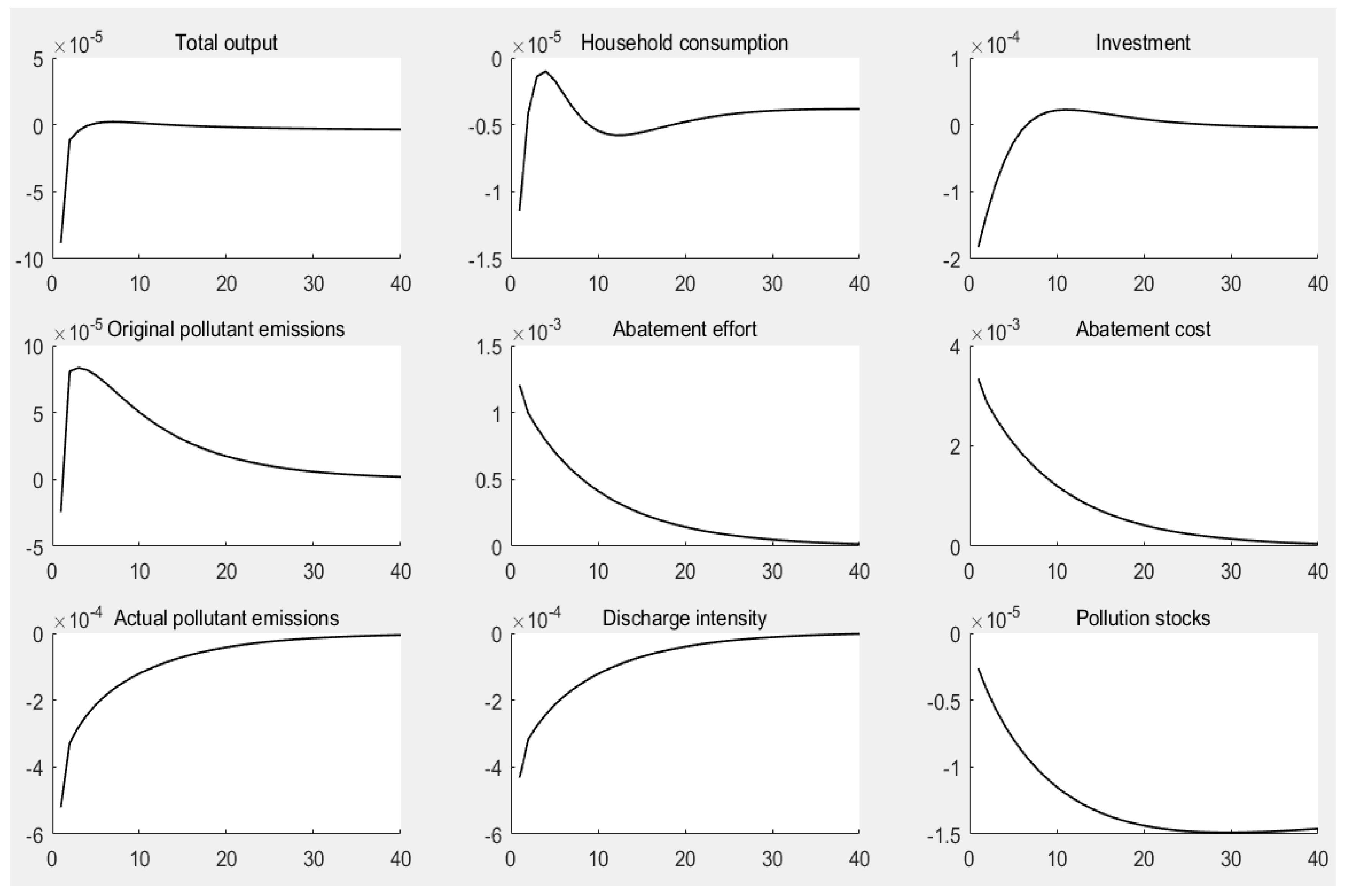
Figure 2 shows the results of a 1% environmental tax rate shock. Firstly, once implemented, the macroeconomic and environmental impacts of an environmental tax policy tend to be largely immediate. Secondly, we found that increasing the environmental tax rate decreased economic activity in terms of investment, household consumption, and overall output. Thirdly, raising the environmental tax rate had the potential to cut pollutant emissions immediately in terms of quantity and intensity, lowering the environmental pollution stock while ultimately having the desired effect of both emission and pollution reduction.

The transmission mechanism of an environmental tax policy on macroeconomic and environmental variables was as follows: (1) In terms of total output, increasing the environmental tax rate increased the pollution discharge cost and total cost to businesses while reducing their productivity. On one hand, this policy not only directly contributed to a decline in business output but also prevented investment and the expansion of business production, ultimately resulting in a decline in total output. On the other hand, the decline in profits caused by the increase in production costs led to a deterioration in the company’s balance sheet, rendering it difficult for the company to finance itself and ultimately leading to a further decline in output levels. (2) In terms of household consumption, when the overall economic output declined, so did the demand from businesses for inputs, which lowered the total household income and consumption levels. (3) In terms of reducing emissions and pollution, increasing the environmental tax rate can limit businesses’ polluting behavior. This will ultimately have a positive impact on the reduction of emissions and pollution. Figure 2 shows that although the original pollutant emissions of businesses increased, with improvements in abatement efforts, the actual pollutant emissions and emission intensity decreased. Finally, considering the ability of the environment to purify itself, the pollution stock decreased. Actually, as the intensity of environmental tax policies rises, the original emissions rise and then fall, while the actual emissions rise and fall. In the early days, the increase in environmental tax rates forced companies to increase their emission reduction efforts, increasing the cost of emissions reduction. However, in order to maximize profits, companies increased their original pollution emissions. Despite the fact that the original pollution emissions have increased, the actual pollution emissions have decreased as a result of increased emission reduction efforts. Afterwards, the original emissions and actual emissions gradually returned to steady-state levels.

5.1.2. Energy Tax Policy Uncertainty

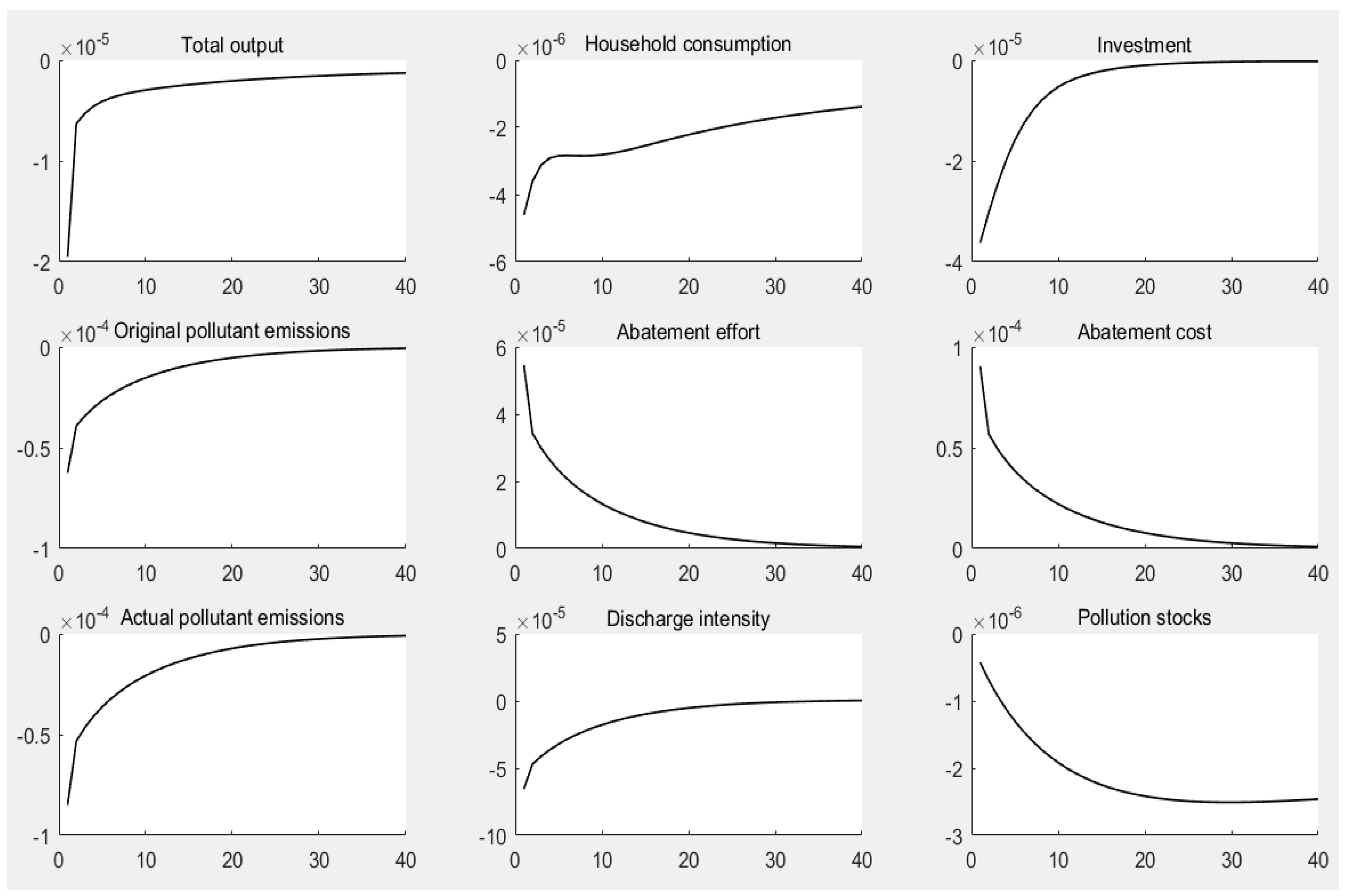
Figure 3 shows the results for a 1% energy tax rate shock. Firstly, the energy tax policy could have an immediate effect across a wide range of variables, but its impact was generally more moderate than that of the environmental tax. Secondly, similar to the environmental tax policy, increasing the energy tax rate also had a restraining effect on social investment, household consumption, and total output. Thirdly, an energy tax policy could reduce emissions and pollution.

The transmission mechanism of the energy tax policy on macroeconomic and environmental variables was as follows: (1) The energy tax policy had two impacts on total output. On one hand, an increase in the energy tax rate led to an increase in energy prices, which increased the cost of energy input and the total cost to businesses and inhibited business production. This restricted capital investment and the expansion of production for businesses at the social level, leading to a decline in total output. On the other hand, the decline in profits caused by the increase in production costs led to a deterioration in the company’s balance sheet, rendering it difficult for the company to finance itself, ultimately leading to a further decline in output levels. (2) In terms of household consumption, increasing the energy tax rate had a restraining effect on economic growth, leading to a decrease in the demand for factors in the household sector from businesses, which in turn resulted in a decrease in the total income of the household sector and, by extension, a decrease in household consumption. (3) In terms of the goal of cutting emissions and pollution, raising the energy tax rate could help to cut emissions and pollution. One way that a higher energy tax reduced emissions was by reducing the energy demand of businesses, which had a direct impact on both the initial and actual emissions of pollutants. However, raising the energy tax rate stimulated businesses to upgrade their manufacturing machinery to increase their ability to reduce emissions, leading to an overall reduction in the inventory of environmental pollutants. It can be seen that the energy tax policy and the environmental tax policy have similar effects. However, as the energy tax policy directly taxes energy consumption, the increase in the intensity of the energy tax policy directly leads to a decrease in output and original pollution emissions.

5.1.3. Emissions Reduction Subsidy Policy Uncertainty

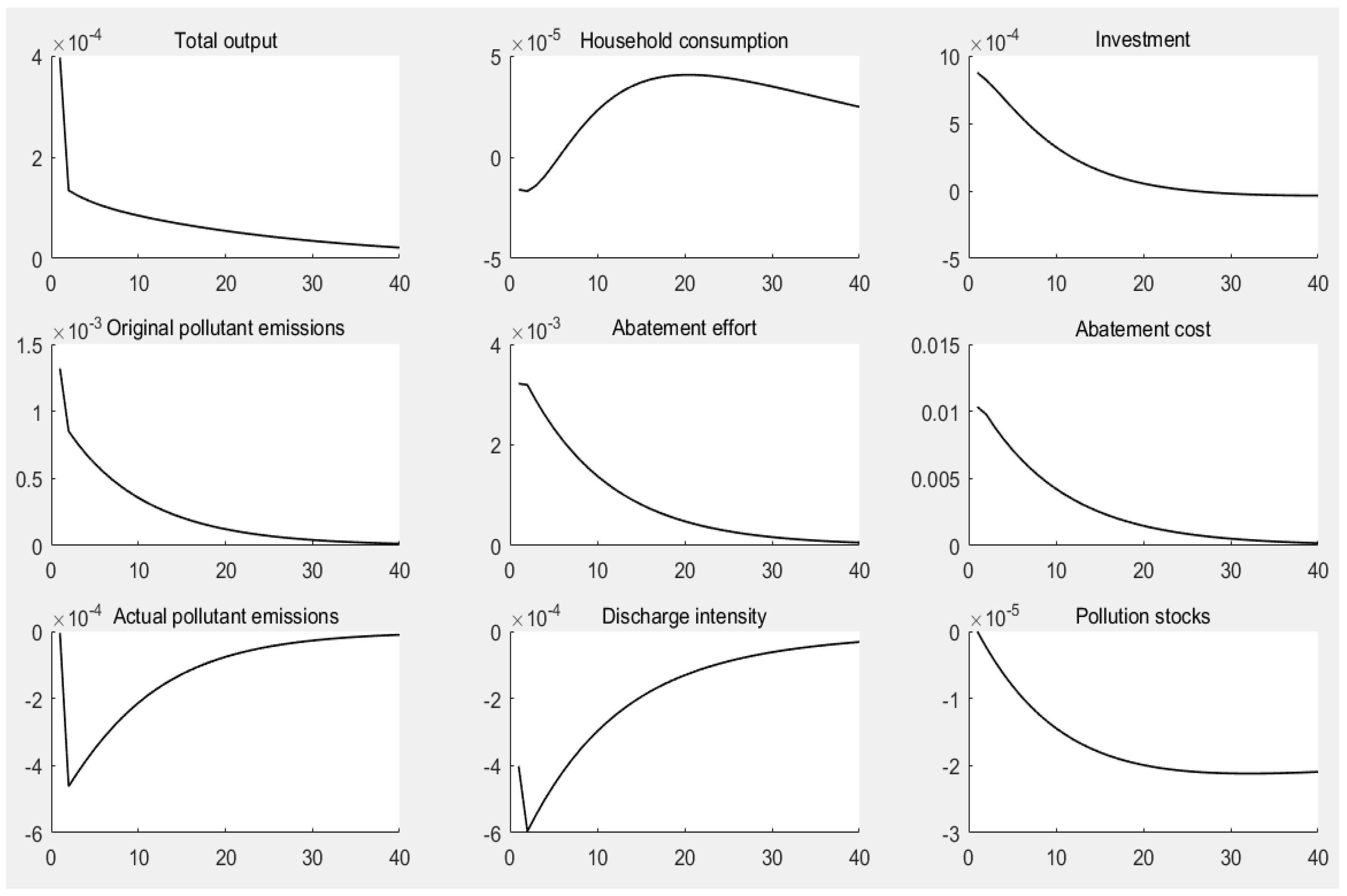
Figure 4 shows the results of a 1% emissions reduction subsidy rate shock. Firstly, increasing the subsidy rate had a significant positive effect on the total output. Secondly, the impact of increasing the subsidy rate for household consumption was initially negative before becoming positive, which had a restricting effect in the short term alongside a promoting effect in the long term. Thirdly, an increase in the subsidy rate reduced actual pollutant emissions, pollution stocks, and emission intensity, resulting in significant emission reduction effects.

The transmission mechanism of subsidy policies on macroeconomic and environmental variables was as follows: (1) The impact of a subsidy policy on total output had two paths. First, an increase in subsidies provided companies with more funds to expand their production scale, which boosted social investment and increased the output level for economic activities. Following the other path, the increase in net profit caused by the increase in subsidies led to an improvement in the company’s balance sheet, rendering it easier for the company to finance itself, leading to a further increase in output levels. (2) The early and late stages of subsidy policies had different effects on household consumption. Initially, an increase in emission reduction subsidies resulted in a relative reduction in household transfer payments and government spending on pollution treatment, whereas a decrease in transfer payments for households resulted in a reduction in total income and consumption. During the later stages, as the economy continued to expand, the demand for input factors from businesses increased. Consequently, both the factor and total income of the household sector increased, with household consumption following suit. (3) An increase in government subsidies for emission reduction helped to achieve the goals of reducing emissions and pollution while also indirectly improving businesses’ ability to raise capital. Businesses are motivated to improve their emission reduction capabilities by updating equipment and technology and improving their management techniques. Finally, even if the original pollutant emissions were increased, the actual pollutant emissions and intensity decreased, leading to a reduction in the pollution stock.

5.1.4. Uncertainty of Government Spending on Pollution Treatment

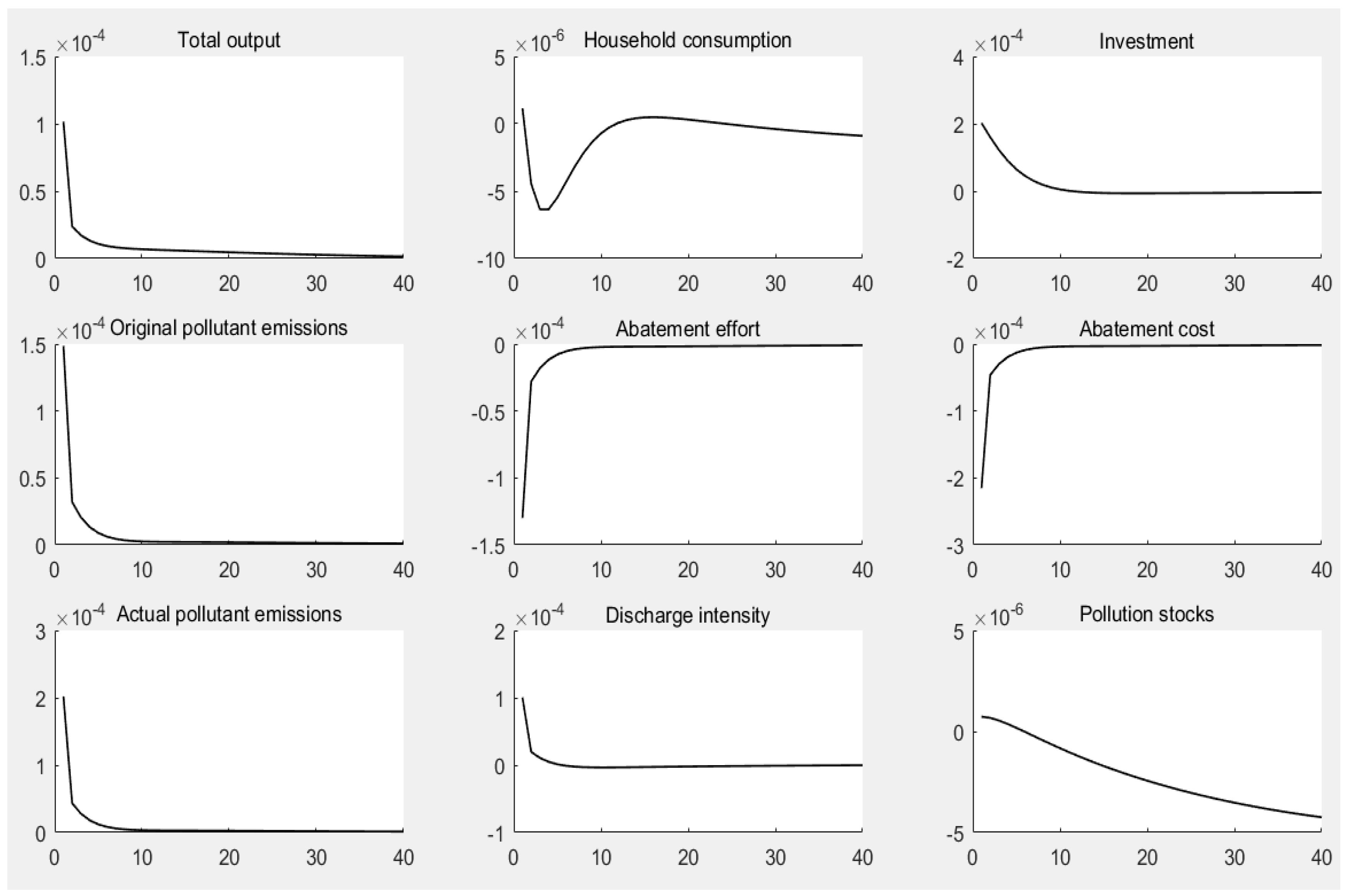
Figure 5 displays the results of 1% government spending on pollution treatment shocks. Firstly, increasing government spending on pollution treatment encouraged the expansion of investments and total output. Secondly, increasing government spending on pollution treatment also had a similar effect on household consumption to that of an emission reduction subsidy policy, which had both short-term deterrent and long-term motivating effects. Thirdly, increasing government spending on pollution treatment had a short-term “pollution reduction” effect rather than a long-term “emission reduction” effect, as it could lower the inventory of environmental pollution while increasing the actual pollutant emissions and intensity.

The mechanism by which government spending on pollution treatment affects macroeconomic and environmental factors operates as follows: (1) In terms of total output, government spending on pollution treatments had three impacts. Firstly, as a part of government purchasing expenditure, the increase in government spending on pollution treatment led to an increase in government purchasing expenditure, which directly drove economic growth from the demand side. Secondly, the increase in government spending on pollution treatment brought about an improvement in environmental quality, which enhanced the labor efficiency of workers and promoted output growth. Thirdly, the improvement in environmental quality reduced the environmental constraints on businesses, leading to a reduction in emission reduction costs, which, to some extent, also promoted output growth. (2) In terms of household consumption, the effect of government spending on pollution treatment was similar to that of subsidy policies; however, it works through different mechanisms. On one hand, the increase in government spending on pollution treatment led to an increase in the price of related products, thereby resulting in a crowding-out effect on private consumption. On the other hand, an increase in government spending on pollution treatment resulted in a relative decrease in transfer payments to the household sector when the size of the government’s welfare expenditure was determined. However, economic expansion increased businesses’ demand for production inputs, which increased households’ total income and consumption levels. (3) Government spending on pollution treatment could have both direct and indirect effects on emission reduction and pollution. Government spending on pollution treatment could reduce environmental pollution directly. However, a decrease in pollution stocks reduced the environmental responsibility of businesses, leading to a decrease in emission reduction efforts alongside an increase in actual pollutant emissions and intensity. In the short term, the indirect effect was greater than the direct effect, resulting in a slight increase in pollution stocks; however, in the long run, the direct effects outweighed the indirect effects, with the stock of environmental pollutants gradually decreasing. Therefore, government spending on pollution treatment only had a “pollution reduction” effect and no “emission reduction” effect.

5.2. Welfare Effects of Green Fiscal and Taxation Policies

Although different green fiscal and tax policies have different focal points, their aim should be to increase the level of social welfare. To give a specific definition, social welfare primarily refers to social support provided to disadvantaged groups with lower incomes, including material and service support. Broadly, this refers to all actions taken to enhance the material and cultural lives of a large number of social members, including good living conditions. Most researchers in economic theory use family objectives or loss functions to gauge the degree of social welfare. Since Ramsey proposed the classical economic man hypothesis, the family objective function has become one of the most widely used techniques and was also used in this study’s analysis of the welfare effects of various green fiscal and tax policies, as shown in Formula (33):

$$\mathit{Welf} = E_0{\sum }_{t=0}^{\infty }{\left(\beta \right)}^t\left\{ln{C}_t-{\mu }_L\frac{{\left(L_t\right)}^{1+\eta }}{1+\eta }-{\mu }_M\frac{{\left({Ea}_t\right)}^{1+\nu }}{1+\nu }\right\}$$

(33)

where $Welf$ represents the level of social welfare. This equation indicates that the level of social welfare is related to household consumption, labor input, and environmental pollutant emissions.

Green fiscal and tax policies have significant impacts on macroeconomic and environmental pollution, which will ultimately be reflected in the level of social welfare (see Figure 6). In addition to emission reduction subsidy policies, policies such as environmental protection taxes, energy taxes, and pollution control expenditures all adversely affect social welfare. The following is a more thorough analysis: (1) Two factors can show how environmental tax policy affects the level of social welfare. Increasing the environmental tax rate reduced pollutant emissions and enhanced social welfare. However, an increase in the environmental tax rate also resulted in lower output levels, household income, household consumption, and levels of social welfare. The level of social welfare ultimately decreased after the second phase, considering that the adverse effects of the environmental tax policy outweighed the favorable effects of the emission reduction policy. (2) The impact of the energy tax policy on the level of social welfare was similar to that of the environmental tax policy, resulting in decreased social welfare. (3) The subsidy policy improved social welfare in two ways. On one hand, the growth effect of the emissions reduction subsidy policy increased the demand for input factors from businesses, which increased the total income and consumption level of households while enhancing social welfare. On the other hand, an emission reduction subsidy policy motivated businesses to reduce pollutant emissions and improve environmental quality, ultimately improving social welfare. (4) There are two steps to explaining how government spending on pollution treatment affects social welfare. During the first stage, from the first to the tenth period, government spending on pollution treatments impacted social welfare through three channels. First, although pollution control spending was able to reduce the stock of environmental pollution, it was not conducive to the improvement of social welfare as it had no “emission reduction” effect. Government spending on pollution treatments led to higher prices for related products, crowding out household consumption and, to some extent, resulting in a loss of social welfare. In addition, an increase in government spending on pollution treatment reduced transfer payments to households in government welfare expenditure, reduced total household income and consumption levels, and, ultimately, resulted in a loss in social welfare. During the second stage, that is, after the 10th stage, with the prominent growth effect of government purchasing expenditure, household income and consumption levels rebounded, and the social welfare level increased again. Nevertheless, the level of social welfare continued to drop because the beneficial impact of government spending on pollution treatments was still lower than its negative impact.

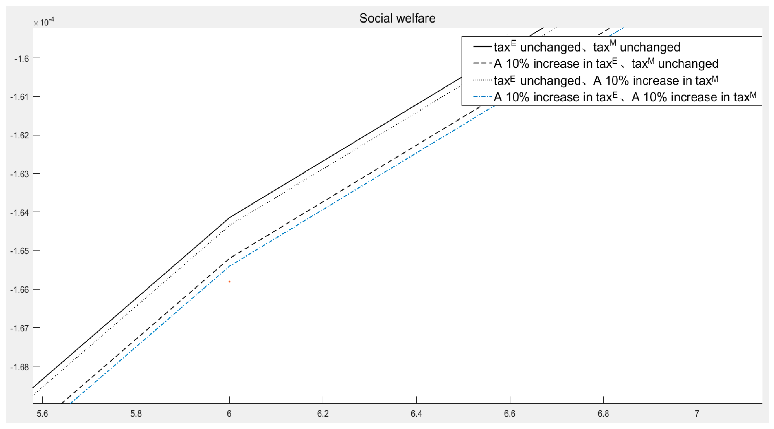
5.3. Further Discussion: Comparing Welfare Losses from Environmental Taxes and Energy Taxes

Evidently, both environmental and energy taxes may cause a loss in social welfare. To compare the impacts of environmental protection and energy taxes on social welfare losses, this study draws on the welfare effects of pollution control expenditures under the four policy combinations (see Figure 7). Case 1 is used as a comparison baseline and implies that the environmental and energy tax rates remained unchanged; in Case 2, the environmental tax rate was increased by 10% while the energy tax rate remained unchanged; in Case 3, the environmental tax rate remained unchanged while the energy tax rate was raised by 10%; and, in Case 4, the environmental and energy tax rates were both increased by 10% simultaneously. It can also be seen from Figure 7 that, compared with Case 1, the social welfare level in the latter three cases had declined to a certain extent, with the decline rate being in the order of Case 3 < Case 2 < Case 4; this indicates that the increase in the environmental tax rate and energy tax would lead to the loss of social welfare, with the policy impact of the environmental tax being greater than that of the energy tax. This is because the energy tax policy only taxed energy consumption, whereas the environmental tax taxed the entire production; thus, the latter had a greater impact. Therefore, increasing the environmental tax rate caused a greater loss to social welfare than that resulting from increasing the energy tax.

5.4. Sensitivity Analysis of the E-DSGE Model

This study examined the sensitivity of the model through the lens of four perspectives, namely, environmental tax, energy tax, emission reduction subsidy, and government spending on pollution treatments. The specific method involved fluctuating the value of each variable by 15% to determine its dynamic impact on total output, household consumption, and actual pollutant emissions to analyze the stability of the model.

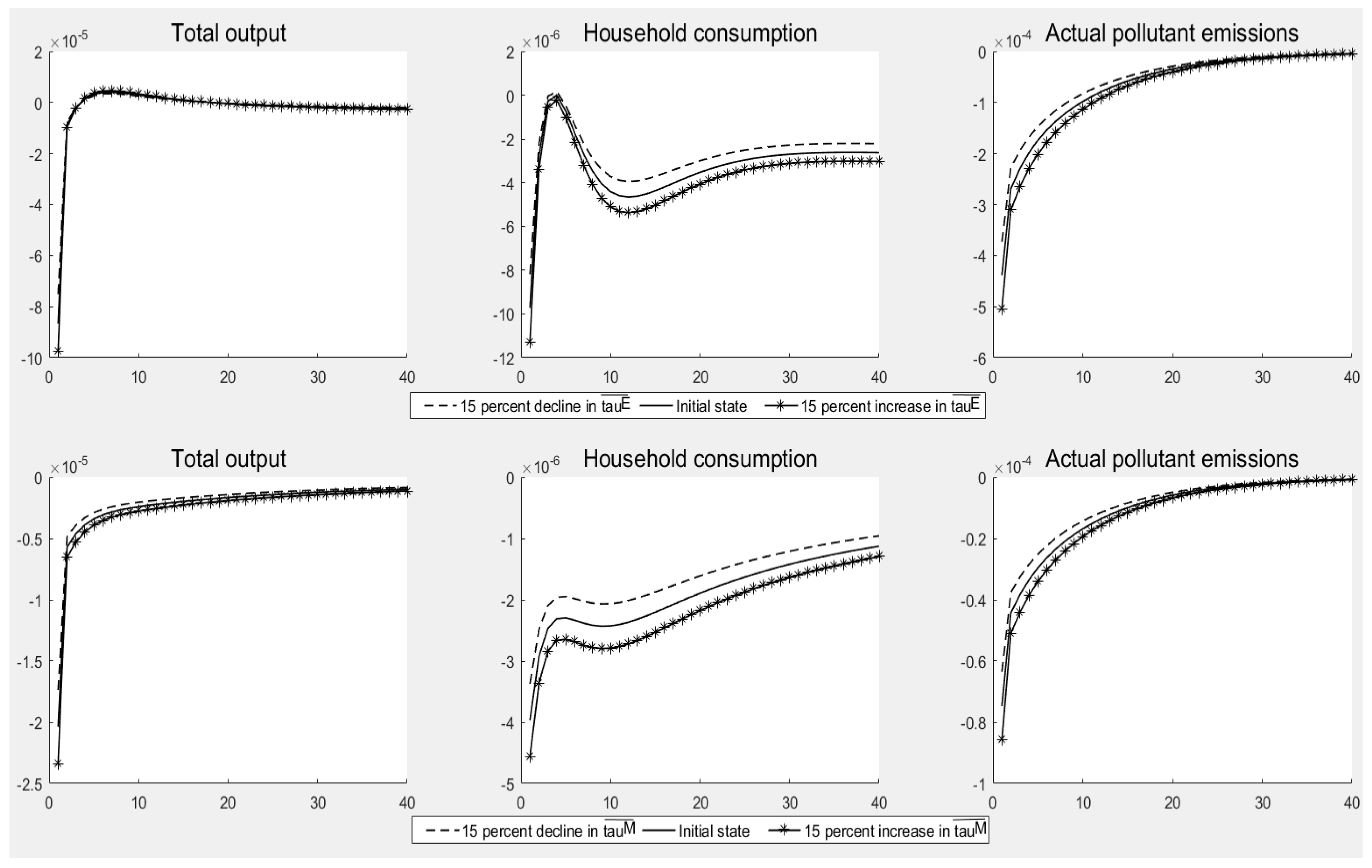
5.4.1. Sensitivity Analysis for Environmental and Energy Tax

Figure 8 shows the dynamic impact of a 15% fluctuation in the environmental tax rate $\overline{{tau}^M}$ and the energy tax rate $\overline{{tau}^E}$ on the major economic and environmental variables. The specific analysis is as follows: (1) Relevant variables may change as the environmental tax rate changes. For instance, a 15% increase in the environmental tax rate had a greater inhibitory effect on total output and household consumption, with the drop in actual pollutant emissions being more noticeable. (2) The result of a 15% fluctuation in the energy tax rate was similar to that of the environmental tax, which is yet to be elaborated upon in detail. (3) Although the pulse response curves for the key variables fluctuated when the values of the environmental and energy tax rates changed, the model remained stable.

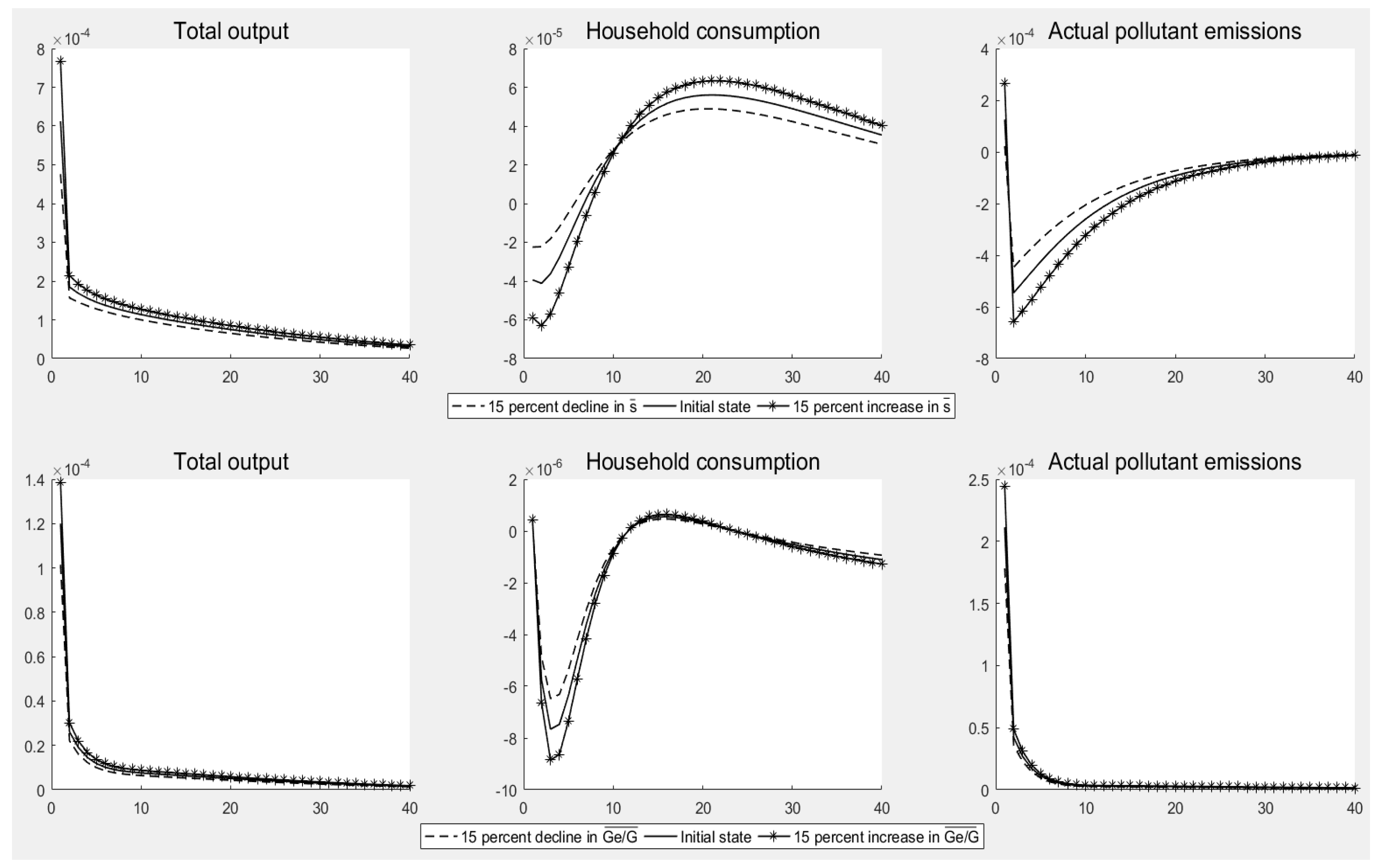
5.4.2. Sensitivity Analysis of an Emission Reduction Subsidy and Government Spending on Pollution Treatments

Figure 9 shows the dynamic impact of a 15% fluctuation in the subsidy rate $\overline{\mathrm{s}}$ and the proportion of government spending on pollution treatments $\overline{G_E/G}$ on the major variables; it provides three pieces of important information. (1) When the emission reduction subsidy rate fluctuated by 15%, the pulse response curve of the main variable also fluctuated. (2) Additionally, the result of a 15% fluctuation in the proportion of government spending on pollution treatment was similar to that for the emission reduction subsidy, although the fluctuation was smaller. (3) Despite the fact that the pulse response curves for the key variables fluctuated when the subsidy rate and the proportion of government spending on pollution treatment were altered, the model remained stable.

6. Conclusions

Green fiscal and tax policies play a key role in promoting sustainable development in China. To study green fiscal and tax policies, we developed an E-DSGE model that contained four major categories of green fiscal and tax policies and subsequently used this model to analyze the economic, environmental, and welfare effects of green fiscal and tax policies. Using this model, the following conclusions could be drawn: (1) Both environmental and energy tax policies could significantly increase businesses’ abatement efforts and reduce actual pollutant emissions, emission intensity, and environmental pollutant stock; however, they restricted the total output and negatively impacted social welfare. Moreover, the policy impact of environmental taxes was more severe than that of energy taxes. (2) The emission reduction subsidy policy not only improved the abatement efforts of businesses and reduced the actual pollutant emissions, emission intensity, and environmental pollutant stock, but also promoted economic growth and improved the level of social welfare, thus creating a “triple win” effect. (3) The emission reduction mechanisms of environmental tax policies, energy tax policies, and subsidy policies are different. Among them, the environmental tax policy and the energy tax policy both reduce pollution by forcing businesses to increase their emission reduction efforts, but the former is a tax on pollution emissions, while the latter is a tax on energy consumption. However, emission reduction subsidy policies incentivize companies to increase their emission reduction efforts and reduce pollution emissions by alleviating their financial burden. (4) Although government spending on pollution treatment could increase the total output while reducing the stock of environmental pollutants, it reduced businesses’ abatement efforts, leading to an overall increase in pollution emissions and intensity. This was because corporations could not be persuaded to reduce their emissions by investing in pollution control [48]. In terms of estimating the level of government environmental spending, the increase in pollution control spending resulted in a reduction in corporate sector subsidies. Therefore, this can be “treated” subsequently rather than “controlled” beforehand, while negatively impacting the improvement of social welfare. (5) An environmental tax would cause greater losses in welfare than an energy tax.

Based on these findings, we propose the following policy recommendations: (1) Although tax-related environmental policies caAn significantly reduce environmental pollution, they should be combined with other incentive-based green fiscal and tax policies, such as subsidies for emission reduction. Environmental tax policies showed a significantly negative impact on social welfare and economic growth. (2) The implementation of higher energy taxes should be prioritized because they have a smaller negative impact on economic growth and social welfare than higher environmental levies. For example, under the 1% energy tax impact, investment, household consumption, and output decreased by 4.16 × 10⁻⁵, 4.35 × 10⁻⁶, and 2.25 × 10⁻⁵, respectively, in the first phase; however, under the 1% environmental tax impact, investment, household consumption, and output decreased by 1.78 × 10⁻⁴, 9.21 × 10⁻⁶, and 8.73 × 10⁻⁵, respectively. In the long run, the impact of a 1% environmental tax policy resulted in a 3 × 10⁻⁴ decline in social welfare, which was greater than the impact of the energy tax policy. (3) Raising emission reduction subsidies could lead to a “triple-win” scenario whereby pollution and emission levels drop alongside improvements in economic growth and social welfare. Consequently, to encourage businesses to engage in green production, subsidies for green production firms and green projects should be enhanced under the current targets of emission reduction, pollution reduction, and “triple pressure”. (4) It is vital to combine incentive-based green fiscal and tax policies, as increasing pollution control expenditures does not encourage businesses to cut emissions or enhance social welfare. (5) Finally, it is essential to develop new pollution control strategies and investigate other types of pollution expenditure that can push businesses to reduce emissions.

Despite the fact that these studies revealed significant discoveries, there are also limitations. (1) Firstly, when building the model, we neglected to account for the differences between green production firms and polluting businesses. (2) Secondly, the model of this paper simplifies the government departments. In fact, the government is also the economic entity that maximizes benefits, and its objective functions may include pollution emissions, GDP growth rate, tax revenue, etc. It is more helpful to include the government utility maximization problem in the model to discuss the reform of green fiscal policy and taxation and the feasibility of tax rates. Unfortunately, we are unable to do it on a technical level. (3) Thirdly, it is worth noting that some important elements were not included, solely on the basis of their being beyond the scope of the study at hand. For example, the impact of conventional environmental regulation policies and green financial policies on green fiscal policies was not considered. (4) Finally, the above conclusions are based on the simulation results of this model, and it is still impossible to compare with the results of other macroeconomic models, such as the CGE model.

China is currently experimenting with various industrial, monetary, and fiscal policies to address environmental issues. The optimal environmental policy to address pressing environmental concerns remains under discussion. Overall, these analyses relate to the Chinese government’s choice of the best policy for reducing pollutant emissions. Future research should also consider the impacts of heterogeneous corporate sectors and different policy combinations on corporate behavior and pollution emissions.

References

- Orlov, A.; Grethe, H.; Mcdonald, S. Carbon taxation in Russia: Prospects for a double dividend and improved energy efficiency. Energy Econ. 2013, 37, 128–140. [Google Scholar] [CrossRef]
- Bovenberg, A.L.; Smulders, S. Environmental quality and pollution-augmenting technological change in a two-sector endogenous growth model. J. Public Econ. 1995, 57, 369–391. [Google Scholar] [CrossRef]
- Itaya, J. Can environmental taxation stimulate growth? The role of indeterminacy in endogenous growth models with environmental externalities. J. Econ. Dyn. Control 2008, 32, 1156–1180. [Google Scholar] [CrossRef]
- Ikefuji, M.; Ono, Y. Environmental policies in a stagnant economy. Econ. Model. 2021, 102, 105574. [Google Scholar] [CrossRef]
- Aydin, L. Potential Economic and Environmental Implications of Diesel Subsidy: A Computable General Equilibrium Analysis for Turkey. Int. J. Energy Econ. Policy 2016, 6, 771–781. [Google Scholar]
- Othman, J.; Yahoo, M. Carbon and energy taxation for CO2 mitigation: A CGE model of the Malaysia. Environ. Dev. Sustain. 2017, 19, 239–262. [Google Scholar]
- Freire-González, J.; Ho, M.S. Carbon Taxes and the Double Dividend Hypothesis in a Recursive-dynamic CGE Model for Spain. Econ. Syst. Res. 2019, 31, 267–284. [Google Scholar] [CrossRef]
- Withey, P.; Sharma, C.; Lantz, V.; McMonagle, G.; Ochuodho, T.O. Economy-wide and CO2 impacts of carbon taxes and output-based pricing in New Brunswick, Canada. Appl. Econ. 2022, 54, 2998–3015. [Google Scholar] [CrossRef]
- Gu, R.; Guo, J.; Huang, Y.; Wu, X. Impact of the EU carbon border adjustment mechanism on economic growth and resources supply in the BASIC countries. Resour. Policy 2023, 85, 104034. [Google Scholar] [CrossRef]
- Constantatos, C.; Pargianas, C.; Sartzetakis, E.S. Green consumers and environmental policy. J. Public Econ. Theory 2021, 23, 105–140. [Google Scholar] [CrossRef]
- He, P.; Qiao, Y.; Long, C.; Yuan, Y.; Chen, X. Nexus between Environmental Tax, Economic Growth, Energy Consumption, and Carbon Dioxide Emissions: Evidence from China, Finland, and Malaysia Based on a Panel-ARDL Approach. Emerg. Mark. Financ. Trade 2019, 57, 698–712. [Google Scholar] [CrossRef]
- Si, S.; Lyu, M.; Lawell, C.Y.C.L.; Chen, S. The effects of environmental policies in China on GDP, output, and profits. Energy Econ. 2021, 94, 105082. [Google Scholar] [CrossRef]
- Wissema, W.; Dellink, R. AGE analysis of the impact of a carbon energy tax on the Irish economy. Ecol. Econ. 2007, 61, 671–683. [Google Scholar] [CrossRef]
- Marinas, M.C.; Dinu, M.; Socol, A.G.; Socol, C. Renewable energy consumption and economic growth. Causality relationship in Central and Eastern European countries. PLoS ONE 2018, 13, e0202951. [Google Scholar]
- Patuelli, R.; Nijkamp, P.; Pels, E. Environmental tax reform and the double dividend: A meta-analytical performance assessment. Ecol. Econ. 2005, 55, 564–583. [Google Scholar] [CrossRef]
- Dechezleprêtre, A.; Sato, M. The impacts of environmental regulations on competitiveness. Rev. Environ. Econ. Policy 2017, 11, 183–206. [Google Scholar] [CrossRef]
- Fischer, C.; Springborn, M. Emissions targets and the real business cycle: Intensity targets versus caps or taxes. J. Environ. Econ. Manag. 2011, 62, 352–366. [Google Scholar] [CrossRef]
- Xiao, B.; Fan, Y.; Guo, X. Exploring the macroeconomic fluctuations under different environmental policies in China: A DSGE approach. Energy Econ. 2018, 76, 439–456. [Google Scholar] [CrossRef]
- Angelopoulos, K.; Economides, G.; Philippopoulos, A. What is the best environmental policy? Taxes, permits and rules under economic and environmental uncertainty. SSRN Electron. J. 2010. [Google Scholar] [CrossRef]
- Heutel, G. How should environmental policy respond to business cycles? Optimal policy under persistent productivity shocks. Rev. Econ. Dyn. 2012, 15, 244–264. [Google Scholar] [CrossRef]
- Annicchiarico, B.; Dio, F. Environmental policy and macroeconomic dynamics in a new Keynesian model. J. Environ. Econ. Manag. 2015, 69, 1–21. [Google Scholar] [CrossRef]
- Wang, R.; Hou, J.; Jiang, Z. Environmental policies with financing constraints in China. Energy Econ. 2021, 94, 105089. [Google Scholar] [CrossRef]
- Pan, X.; Xu, H.; Li, M.; Zong, T.; Lee, C.T.; Lu, Y. Environmental expenditure spillovers: Evidence from an estimated multi-area DSGE model. Energy Econ. 2020, 86, 104645. [Google Scholar] [CrossRef]
- Wu, X. On the dynamic effect of environment protection technology, energy saving and emissions reduction policy on ecological environment quality and transmission mechanism: Simulation analysis based on three-sector DSGE model. Chin. J. Manag. Sci. 2017, 25, 88–98. [Google Scholar] [CrossRef]
- Cai, D.; Yan, Y.; Cheng, S. Research on the impact of carbon emission subsidies and carbon taxes on environmental quality. China Popul. Resour. Environ. 2019, 29, 59–70. [Google Scholar]
- Punzi, M.T. Role of Bank Lending in Financing Green Projects: A Dynamic Stochastic General Equilibrium Approach; Working Papers; Asian Development Bank Institute: Tokyo, Japan, 2018. [Google Scholar]
- Wang, Y.; Pan, D.; Peng, Y.; Liang, X. China’s incentive policies for green loans: A DSGE approach. J. Financ. Res. 2019, 11, 1–18. [Google Scholar] [CrossRef]
- Liu, L.; He, L. Output and Welfare Effect of Green Credit in China: Evidence from an estimated DSGE model. J. Clean. Prod. 2021, 294, 126326. [Google Scholar] [CrossRef]
- Dixit, A.K.; Stiglitz, J.E. Monopolistic competition and optimum product diversity. Am. Econ. Rev. 1977, 67, 297–308. [Google Scholar]
- Calvo, G.A. Staggered prices in a utility-maximizing framework. J. Monet. Econ. 1983, 12, 383–398. [Google Scholar] [CrossRef]
- Frankenberg, E.; McKee, D.; Thomas, D. Health Consequences of forest fires in Indonesia. Demography 2005, 42, 109–129. [Google Scholar] [CrossRef]
- Pönkä, A. Absenteeism and respiratory disease among children and adults in Helsinki in relation to low-level air pollution and temperature. Environ. Res. 1990, 52, 34–46. [Google Scholar] [CrossRef] [PubMed]
- Zivin, J.G.; Neidell, M. The impact of pollution on worker productivity. Am. Econ. Rev. 2012, 102, 3652–3673. [Google Scholar] [CrossRef] [PubMed]
- Deng, K.; Zeng, H. The financial constraints in China. Econ. Res. J. 2014, 49, 47–60+140. [Google Scholar]
- Kiyotaki, N.; Moore, J. Credit cycles. J. Pol. Econ. 1997, 105, 211–248. [Google Scholar] [CrossRef]
- Iacoviello, M. House prices, borrowing constraints, and monetary policy in the business cycle. Am. Econ. Rev. 2005, 95, 739–764. [Google Scholar] [CrossRef]
- Li, X. Dynamic Stochastic General Equilibrium (DSGE) Model: Theory, Methodology, and Dynare Practice; Tsinghua University Press: Beijing, China, 2018; p. 34. [Google Scholar]
- Zhu, J. Advanced Public Finance 2: DSGE’s Perspective and Frontiers in Application: Model Decomposition and Programming; Shanghai University of Finance and Economics Press: Shanghai, China, 2019; p. 5. [Google Scholar]
- Wu, H.; Xu, Z.; Hu, Y.; Yan, P. Fiscal policy and its macro impact under the impact of news. Manag. World 2011, 12, 26–39. [Google Scholar]
- Bian, Z.; Yang, Y. Structural fiscal policy regulation and fiscal tools choice in the new normal. Econ. Res. J. 2016, 51, 66–80. [Google Scholar]
- Blanchard, O.; Galí, J. Labor markets and monetary policy: A new Keynesian model with unemployment. Am. Econ. J. Macroecon. 2010, 2, 1–30. [Google Scholar] [CrossRef]
- Nalban, V. Forecasting with DSGE models: What frictions are important? Econ. Modell. 2018, 68, 190–204. [Google Scholar] [CrossRef]
- Pop, R. A small-scale DSGE-VAR model for the Romanian economy. Econ. Modell. 2017, 67, 1–9. [Google Scholar] [CrossRef]
- Nordhaus, W.D. To slow or not to slow: The economics of the greenhouse effect. Econ. J. 1991, 101, 920–937. [Google Scholar] [CrossRef]
- Falk, I.; Mendelsohn, R. The economics of controlling stock pollutants: An efficient strategy for greenhouse gases. J. Environ. Econ. Manag. 1993, 25, 76–88. [Google Scholar] [CrossRef]
- Huang, Z.; Zhu, B. Real business cycles and taxation policy’s effects in China. Econ. Res. J. 2015, 50, 4–17+114. [Google Scholar]
- Ministry of Finance of the People’s Republic of China. Notice on Policies on Degenerate VAT Rates, 2017. Available online: https://www.chinatax.gov.cn/chinatax/n810341/n810765/n2511651/201704/c2712766/content.html (accessed on 8 January 2024).
- Han, C.; Wang, Z. Alternatives for emissions reduction other than regulation: Evidence for emissions reduction driven by opening up to foreign investment. Fin. Trade Econ. 2022, 43, 97–113. [Google Scholar]
Figure 1.
Basic framework of E-DSGE model.
Figure 2.
Pulse response to an environmental tax rate shock.
Figure 3.
Pulse response of an energy tax rate shock.
Figure 4.
Pulse response to an emission reduction subsidy rate shock.
Figure 5.
Pulse response to a shock from government spending on pollution treatments.
Figure 6.
Welfare effect of green fiscal and taxation policies.
Figure 7.
Welfare effects of a shock from government spending on pollution treatments under different green tax combinations.
Figure 8.
Sensitivity analysis of environmental taxes and energy taxes.