A Dimensionless Study Describing Heat Exchange through a Building’s Opaque Envelope

Abstract

The urban environment represents one of the main contexts in which natural resources are exploited to support intensive human activities, especially from an energy perspective. In this context, there is still a lack of general methodologies/tools which can be used to understand the behavior of buildings and to prove their sustainability under real operating conditions, depending on their location, construction characteristics and materials, plants, external conditions, and conduction. In this research, the Buckingham theorem is applied to the thermophysics of buildings, describing the heat transfer of opaque surfaces in a transient regime. The abstraction of dimensionless numbers merges the main phenomena of interest, such as thermal conduction, convection, and radiation, enhanced by consideration of the surface sun–air temperature and the external air temperature. The parameters themselves were mutually matched through a proper equation, whose coefficients were determined by a regression analysis of the measurements from an intensive experimental campaign investigating a building in Florence for 3 years. The resulting correlation shows a good agreement with the available dataset and a determination coefficient of over 70%. Therefore, the proposed approach, owing to the generalization of the dimensionless numbers, suggests the possibility of sustainability estimates, from an energy point of view, of envelope/plant/user systems, including assessments at a higher scale than that of a single building.

1. Introduction

Given the high energy consumption and greenhouse gas emissions resulting from the construction sector, buildings play a key role in achieving a sustainable, competitive, secure, and decarbonized energy system in the European Union [1]. A thorough understanding of the thermodynamics of buildings and their components is needed to provide energy-efficient buildings [2]. In particular, the accurate assessment of the real heat exchange in situ is fundamental for the characterization of the real dynamic behavior of building components [3].

Along these lines, heat flux measurement techniques have been advanced and integrated over the years [4,5,6]. Flanders [7] reviewed the use of heat flux transducers for in situ measurement of building performance. He provided key insights for the proper calibration, thermal matching, and accounting for lateral heat flow and thermal lags in in situ data. As regards calibration, Zarr et al. [8] compared different calibration processes for a thin heat flux sensor for building applications. They showed that the calibration using Test Methods C 177 [9] and C 518 [10] can be considered statistically equivalent for several applications. Alternatively, Pullins and Diller [11] developed a new wide-angle radiation calibration system needed for the calibration of high-temperature heat flux sensors (HTHFS), i.e., sensors capable of simultaneously measuring thermopile surface temperature and heat flux in extreme thermal environments (up to 1000 °C). HTHFS were designed, fabricated, and subsequently characterized by Zhang et al. [12]; in particular, thin film thermopile (TFTP) heat flux sensors by surface micromachining technology were described. When using silicon oxide as the thermal insulator, the TFTP could work at 1000 °C, while with spin coated polyimide, it could be used at temperatures of up to 400 °C. On the other hand, Langley et al. [13] developed a versatile, flat, surface-attached heat flux sensor using photoimageable dielectrics for patterning, as well as innovative polymer-based materials. Their applications included insulation testing, fire detection, etc. Similarly, a textile heat-flux sensor made using different woven fabric materials was produced and analyzed in [14]. All the developed textile heat flux sensors showed sensitivities equivalent to their existing commercial counterparts. However, the sensors made with a ratio of 70/30 of polyester and cotton, respectively, demonstrated the highest sensitivity, for both large and small sizes. On the contrary, other studies have studied alternative techniques for minimizing the influences of the measurement apparatus and the boundary conditions on the heat flow through the surface. For instance, Saidi and Kim [15] proposed a heat flux sensor that measures both heat transfer and temperature with minimal effect on the wall’s thermal boundary condition since the passive temperature sensor is very thin. Cucumo et al. [16] studied the degree to which the heat flux of external walls is deflected by heat flux sensors due to their different thermal conductivity. The results show that the error is lower for well-insulated walls but significant for a wall with high conductance. Biddulph et al. [17], instead, proposed a method to estimate the in situ thermal transmittance and thermal mass of a building wall which was less time-consuming and seasonally bounded than the standard steady-state method [18]. This method combines a simple physical model of the building element, based on electrical analogy, with Bayesian analysis. It has been demonstrated to provide the same results as the steady-state method, but while significantly reducing the length and limitations of the monitoring period needed since it uses dynamic temperature changes, rather than requiring a high temperature difference. Similarly, Rasooli and Itard [19] proposed modifications to the standard heat-flow meter method [18] using an additional heat flux sensor, placed opposite to the first one, which allows the observer to obtain the thermal transmittance with a higher precision in a shorter period of time.

These various approaches can be used to characterize the thermophysical properties of building components and materials, both in situ and in the lab. Distefano et al. [20] used thermophile sensors, combined with two heating/cooling plates, to define the thermal conductivity and thermal resistance of a panel made up of alveolar corrugated cardboard. Similarly, Baccilieri et al. [21] applied Test Method C 518 [10] to characterize the thermal conductivities of various structures fully made up of natural and biocompatible materials by a heat-flow meter apparatus that establishes a steady-state one-dimensional heat flux through a test specimen placed between two parallel plates at different constant temperatures. Cardinale et al. [22,23] utilized the same heat-flow meter apparatus to identify in the lab the thermal performance of cement mortar with reed and straw fibers or PVC compound additive. On the other hand, Cesaratto and De Carli [24] analyzed different methods to measure the in situ thermal conductance of building components under real conditions, but always following the standard heat-flow meter method [18]. The results highlighted that this method could give significantly different results for the same case, depending on various factors, namely the sensitivity to dynamic conditions in the input data, or the initial thermal field inside the measured element.

To understand the heat exchange mechanism through building components, experimental data, simulation results, and/or numerical analysis are required. However, empirical data on energy performance for constructive solutions and different climate boundary conditions are often not available. Therefore, a few studies have used dimensional analysis [25] to provide an alternative widely accepted as valid to describe the thermal-energy performance of building components. Indeed, this analytical technique allows the description of physical and thermodynamic processes by dimensionless variables [26]. For instance, Balocco [26] proposed a method for studying the energy performance of naturally ventilated double façades based on the definition of 14 non-dimensional numbers starting from the thermophysical characteristics of the façade. This method can support building designers by providing the heat flux through the wall as a function of simple parameters without the need for complex simulations. Wang et al. [27], instead, applied the dimensionless method to study the adaptive thermal control of positive temperature coefficient (PTC) material. They obtained a fitting equation to estimate the equilibrium temperature of a controlled device that can be applied to ceramic PTC materials with good accuracy. Trethowen [28] used a dimensionless parametric model to further different purposes by quantitatively predicting the magnitude of errors associated with measurements of building heat flows through surface-mounted sensors. The model, based on finite-difference computer predictions, allows for the characterization and comparison of the error levels of different heat flux sensors, depending on the operating conditions.

In this framework, the present research aims to provide a useful tool that allows the evaluation of the weight of the fundamental parameters within the temporary value of the heat flow at unsteady conditions and, prospectively, to compare the thermophysical performance of different opaque wall configurations. The objective is to find the link between the thermophysical behavior expressed through heat exchange and the real characteristics of any typology of a building wall, and the thermal stresses due to internal and external forcing at operative dynamic conditions.

In detail, the present study describes the heat exchange through the wall by extrapolating a dimensionless analysis based on the Buckingham π theorem [29]. Therefore, through the application of such a methodology, an effective correlation among the dimensionless numbers was found, as approximated with a set of experimental data.

These data were obtained by an intensive measurement campaign carried out on a pilot building in Florence. By means of this measurement campaign the thermal flux passing through a building’s opaque walls at real transient conditions was continuously monitored and measurements acquired during several years (this research was published in [30]), as summarized in the following (Section 2.2).

Then, the obtained correlation allows for the most correct and coherent interpretation possible of the heat exchange in real transient conditions. The results show how, thanks to the dimensional analysis and the correlation obtained, it is possible to study the behavior and thermophysical performance of any building wall, taking into account the variability of external and internal loads, to identify possible energy-efficiency solutions by starting with a simple tool of evaluation. In line with this purpose, Zhang et al. [31] suggested the development of genetic algorithms aiming at optimal solutions for energy consumption and thermal comfort. Proposed strategies on the Pareto frontier suggested significant energy savings. Especially, by incorporating occupant behavior, a potential energy reduction of up to about 20% could be achieved, emphasizing the importance of considering human factors in building energy efficiency designs. Natarajan et al. [32], instead, focused attention on the importance of using deep learning models for merging neural networks with long short-term memory data and IoT-enabled smart meter data, which offers significant potential for guiding tailored energy management strategies in both residential and commercial spaces.

2. Materials and Methods

2.1. The Analytical Model

The proposed research is based on the application of the Buckingham π theorem in the field of building thermophysics, aiming at the description of dynamic thermal loss through opaque walls depending on different boundary conditions and material properties.

The π theorem originates from the study of dimensional analysis in fluid-dynamics issues, proving to be an effective tool widely used for processing correlations among experimental data of highly complex phenomena. This theorem ensures the reduction of the number of variables appearing in the relationship describing a phenomenon thanks to the definition of an equivalent equation among a more limited number of dimensionless numbers [33]. A generic dimensional homogeneous relationship can be written in the following form:

$$f\left(x_1, x_2, x_3, \dots , x_{\mathrm{n}}\right)=0$$

(1)

where $x_1$ is the dependent variable and the remaining $x_{\mathrm{n}-1}$ parameters are independent variables, so that an equivalent relationship exists in the following form:

$$F\left({\mathsf{\Pi }}_1, {\mathsf{\Pi }}_2, \dots , {\mathsf{\Pi }}_{\mathrm{n}-\mathrm{j}}\right)=0$$

(2)

where 1, 2, …, n − j, are dimensionless values derived from a combination of independent and dependent variables. The variable j represents the total number of fundamental dimensions considered, each taken into account at most once. It then can be said that the following number of dimensionless parameters z results:

$$\mathrm{z}=\mathrm{n}-\mathrm{j}$$

(3)

In the present case, the method was developed and applied to the heat exchange phenomenon in the building envelope as a function of its material properties and the indoor/outdoor dynamic boundary conditions. The dimensionless analysis approach, which is a robust instrument widely used in physical and engineering sciences, provides the possibility of generalizing any physical phenomenon, avoiding the dependence on the specific components and/or parameters’ properties and local outdoor/indoor climatic constraints.

First of all, the proposed method introduces the process of matching the suitable information to be collected in a real context. Therefore, it shows how to combine them to derive the characteristic dimensionless numbers according to the Buckingham theorem application (also known as the Pi theorem). Finally, the method proposes a correlation, validated through an experimental campaign, which is used to find the expected heat flux occurring through an opaque wall, as connected to the envelope’s thermophysical characteristics and the indoor and outdoor climatic parameter variations. Accordingly, this approach allows one to describe the building’s performance and to address its sustainability.

Considering the heat exchange that affects a wall, 9 independent variables may be chosen to describe it and to obtain the dependent variable named real heat flux q [W/m²], which describes the heat flux passing through the wall itself in dynamic conditions:

• Wall thickness s_w [m];
• Wall thermal resistance R_w depending on its stratigraphy [m² °C)/W];
• Indoor air temperature T_in [°C];
• Wall outdoor surface temperature T_ew [°C];
• Solar radiation hitting the external surface of the wall I_⊥ [W/m²], perpendicularly;
• Air mass flow m_a [kg/s], blowing to the external surface of the wall because of the presence of wind, perpendicularly;
• Thermal conductivity of outdoor air k_a [W/m °C]
• Specific heat at constant pressure of air c_p [kJ/(kg °C)];
• Dynamic viscosity of air μ_a [kg/(m s)].

Then, with the overall 10 variables and the 4 fundamental unit dimensions [kg, m, s, and °C] the number of dimensionless numbers comes to 6 (N₁, N₂, N_n, …, N₆).

The dimensionless number N₁ represents the thermal flux passing through the wall in quasi-steady-state conditions (meaning that the thermophysical properties of the media and fluids do not change as the temperature varies) as a function of the external air conditions. Inside N₁ the thermal flux is expressed as a function of the total thermal transmittance of the wall and the difference between the internal and external surface temperature, and can be expressed as follows:

$$N_1=\frac{q_c · s_w}{k_a·\mathsf{\Delta }{T}_{ }}$$

(4)

where q_c is the thermal flux [W/m²] calculated as a function of the difference in temperature ΔT [°C] between the external wall temperature T_ew and the indoor temperature T_in [°C]. So q_c could be written by the following:

$$q_c=\frac{T_{ew}-T_{in}}{R_w+\frac{1}{h_{in}}}$$

(5)

with h_in the indoor surface coefficient for heat convective heat exchange [W/(m² °C)].

The external wall temperature is evaluated as the sun–air temperature, including the contribution of the solar radiation hitting the façade:

$$T_{ew}=T_{out}+\left(\frac{\alpha ·{ I}_{\perp }}{h_{out}}\right)$$

(6)

where I_⊥ is the solar radiation hitting the external surface of the wall perpendicularly, α is the average hemispherical coefficient of absorption of the wall due to the finishing and painting, and h_out is the outdoor surface coefficient for convective heat exchange [W/(m² °C)].

The second number according to the Buckingham theorem is related to the convective heat exchange contribution due to the external air hitting the wall perpendicularly:

$$N_2=\frac{m_a · c_p}{k_a · s_w}$$

(7)

where m_a is the air mass flow [kg/s] blowing to the external wall because of the presence of wind for the area of the tile sensor A_t (v_⊥ is the normal component of wind velocity):

$$m_a={\rho }_a{ · v}_{\perp }{ · A}_T$$

(8)

The remaining dimensionless numbers were set to match the other variables chosen for the analysis and are listed below:

• N₃ represents the inertial forces with respect to the friction-based ones for the fluid air (the same as Reynolds’ number):

$$N_3=\frac{m_a}{{\mu }_a · s_w}$$

(9)

• N₄ links the heat transfer due to the conduction of external air with the total thermal resistance of the wall:

$$N_4=\frac{k_a · R_w}{s_w}$$

(10)

• N₅ represents the heat transfer of the wall with respect to the incoming solar radiation:

$$N_5=\frac{k_a · \mathsf{\Delta }T}{s_w · I_{\perp }}$$

(11)

• N₆ synthetizes the specific differences of temperature, scaled with the temperature of the external wall surface:

$$N_6=\frac{\mathsf{\Delta }T}{T_{ew}}$$

(12)

The six dimensionless numbers were then finally combined together in an equation with the following general form:

$$N_1^{*}=a ·{ N}_1^b · N_2^c · N_3^d · N_4^e · N_5^f · N_6^g$$

(13)

where a, b, c, d, e, f, and g are the unknown coefficients that need to be determined and $N_1^{*}$ represents the real dynamic heat flux through the wall with respect to the heat transfer due to the flow field of the external air. It expresses the parameter to be found for evaluating the energy performance and sustainability of a building, and can be written as

$$N_1^{*}=\frac{q · s_w^2}{m_a · c_p· \Delta T}$$

(14)

Moreover, the correlation may be linearized through the properties of logarithms, simplifying the correlation algorithm, as

$$ln\left(N_1^{*}\right)=ln\left(a\right)+b · ln \left(N_1\right)+c · ln \left(N_2\right)+d · ln \left(N_3\right)+e · ln \left(N_4\right)+f · ln \left(N_5\right)+g · ln \left(N_6\right)$$

(15)

2.2. Validation of the Correlation through an Experimental Monitoring Campaign at a Real Site

To evaluate the correlations among the dimensionless numbers with the proper values of the coefficients, an experimental campaign based on environmental measurements of a real building in Florence was used. In this case study, the thermo–hygrometric parameters of the indoor and the corresponding external conditions were continuously monitored from 2017. The building complex, owned by Casa Spa (a subsidiary of the Florence municipality), complies with the Nearly Zero Energy Building (nZEB) requirements [34]. The structure is made of wood (XLAM) and thanks to proper insulation (glass/rock wool layers), a declared total energy consumption of 16 kWh/m² per year is reached.

The monitoring system, designed for a decade-long integration into living spaces, employed common commercial transducers for air temperature (T_in [°C]) and relative humidity (RH_in [%]) measurements on internal walls. Additionally, a dozen flux tiles developed at the University of Florence were installed on outer walls facing southwest [30]. These tiles directly measured transient heat flux (q_m [W/m²]), considering external parameter fluctuations and the thermophysical properties of building materials.

Tile sensors, fixed to the wall, rapidly responded to impulsive stresses, capturing indoor air temperature variations within minutes. The output signal of each tile sensor, proportional to the thermal flux passing through it, is linked to the temperature difference between opposing surfaces. The relative measurement error for this device is 3.5% and the thermal resistance R_t is 0.001 (m² °C)/W, with an active area of 0.45 × 0.45 m². The installation collected signals through shielded cables running within special ducts under the plaster, reaching the fifth floor, where a commercial analogue data logger is located [30].

The measuring campaign carried out for this existing building in Florence lasted 3 years, and the post-processing approach of all the data has been described in [30]. Considering the building’s thermophysics and the scale of investigation, the hourly variation of any parameter makes sufficient physical sense. Consequently, the experimental data were aggregated with this time step, aiming at quantifying the physical variables and parameters of interest and the derived dimensionless numbers. The data were controlled and filtered by a Virtual Basic (VB) script within Excel™ 2021 to ensure the physical and mathematical significance of the values of the dimensionless numbers obtained and the correlations among them. The experimental conditions that provided null values and indeterminacy of the related dimensionless number were not considered. Similarly, the negative results were not taken into account, since the function is linearized through the use of the natural logarithm (the domain considers only positive values in the arguments). According to these assumptions, the correlation function was obtained with a dataset of 64 valid samples that were considered statistically representative for the evaluation of the 7 coefficients.

In the left side of Equation (13), the thermal flux measured during the experimental campaign q_m was used in substitution of q to obtain the vectors of the real values for the number $N_1^{*}$:

$$N_1^{*}=\frac{q_m · s_w^2}{m_a · c_p· \mathsf{\Delta }T}$$

(16)

Also, N₁ was updated to consider the presence of the tile sensor, adding the contribution of its thermal resistance R_t inside the thermal flux q_c (Equation (5)), and achieving $q_c^{\prime }$:

$$q_c^{\prime }=\frac{T_{ew}-T_{in}}{R_w+\frac{1}{h_{in}}+R_t} .$$

(17)

Beyond the thermal flux passing through the investigated walls, other known parameters were considered in describing the overall heat exchange phenomena and in the calculation of the dimensionless numbers of the previous section. Some of the variables, including those related to the geometry and material properties, were assumed to be constant in time (with the temperature variation), such as the following:

• Wall thickness s_w equal to 0.325 m;
• Wall thermal resistance R_w equal to 6.25 (m² °C)/W;
• Main surface of the tile sensor A_t of 0.2025 m² (reference area for the thermal flux);
• Thermal resistance of the tile sensor R_t equal to 0.001 (m² °C)/W;
• Internal heat transfer coefficient for indoor natural convection h_in equal to 8 W/(m² °C) [35];
• External heat transfer coefficient for outdoor natural convection h_out equal to 23 W/(m² °C) [35];
• Average hemispherical coefficient of absorption α of the wall fixed at 0.5 [-] (reliable value for the investigated building).

It is important to notice that, in the described case, the thermal resistance of the tile sensor could be neglected in Equation (17) because of the high thermal insulation of the studied wall (R_t << R_w). However, the technical–constructive features of the tile sensor produce a disturbing effect on the heat flux that passes through and is distributed in the different layers of wall materials. This fact is also proven by other research works, i.e., [28,36,37].

Other variables, those related to the external environment, were determined by weather stations and are available in the territory from LaMMA (Laboratory for Meteorology and Environmental Modelling [38]) and the University of Florence:

• Outdoor temperature T_out [°C];
• Outdoor relative humidity RH_out [%];
• Wind velocity w_v [m/s];
• Wind direction w_dir, clockwise from North [°];
• Atmospheric pressure p_a [Pa];
• Direct DNI and global G solar radiation [W/m²].

The outdoor temperature was then used to derive some variables referred to the external air, thanks to the software EES™ 10.836, which is based on the equations provided by ASHRAE [39]:

• Thermal conductivity k_a [W/(m °C)];
• Specific heat at constant pressure c_p [kJ/(kg °C)];
• Dynamic viscosity μ_a [kg/(m s)];
• Density ρ_a [kg/m³].

Instead, the measured solar radiation was elaborated to find the solar radiation load hitting the wall I [W/m²] and the surface sun–air temperature T_ew [°C], while the wind direction and velocity were used to estimate the air mass flow m_a impacting it. In the case study, the wall is oriented with an angle of 39° to the south toward the west direction, determining the definition of the hourly perpendicular component of solar radiation I_⊥ and wind velocity v_⊥ through the effect of the incident angle cosine.

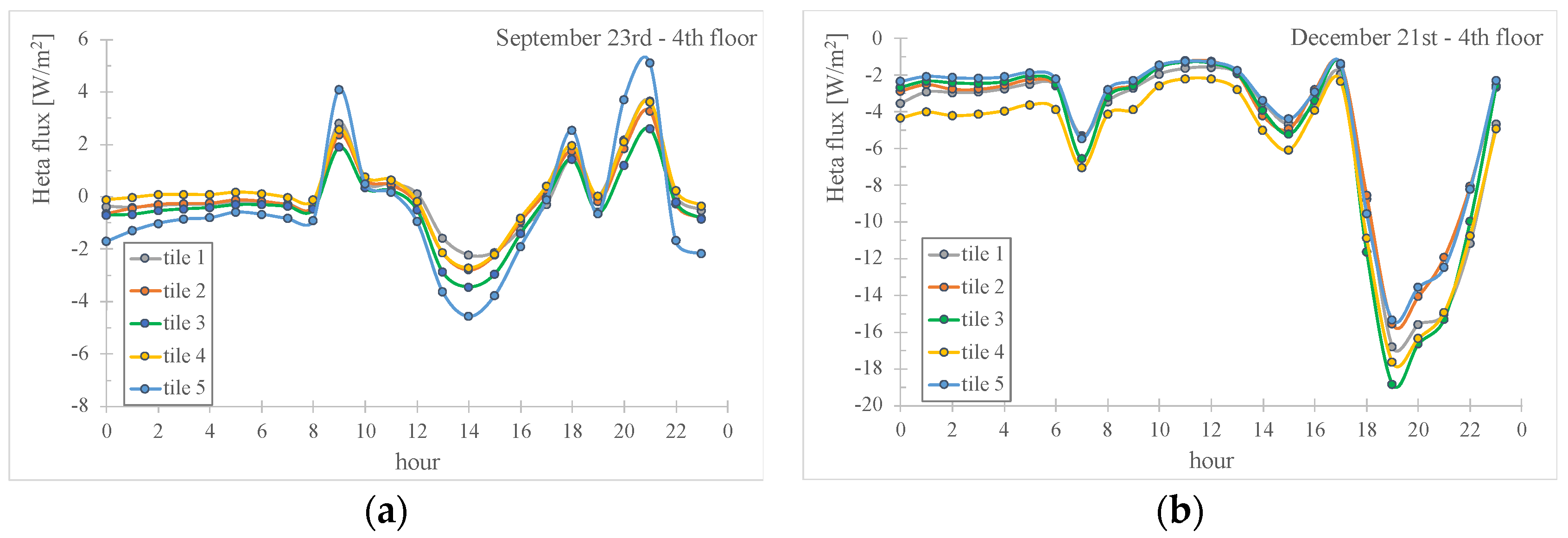
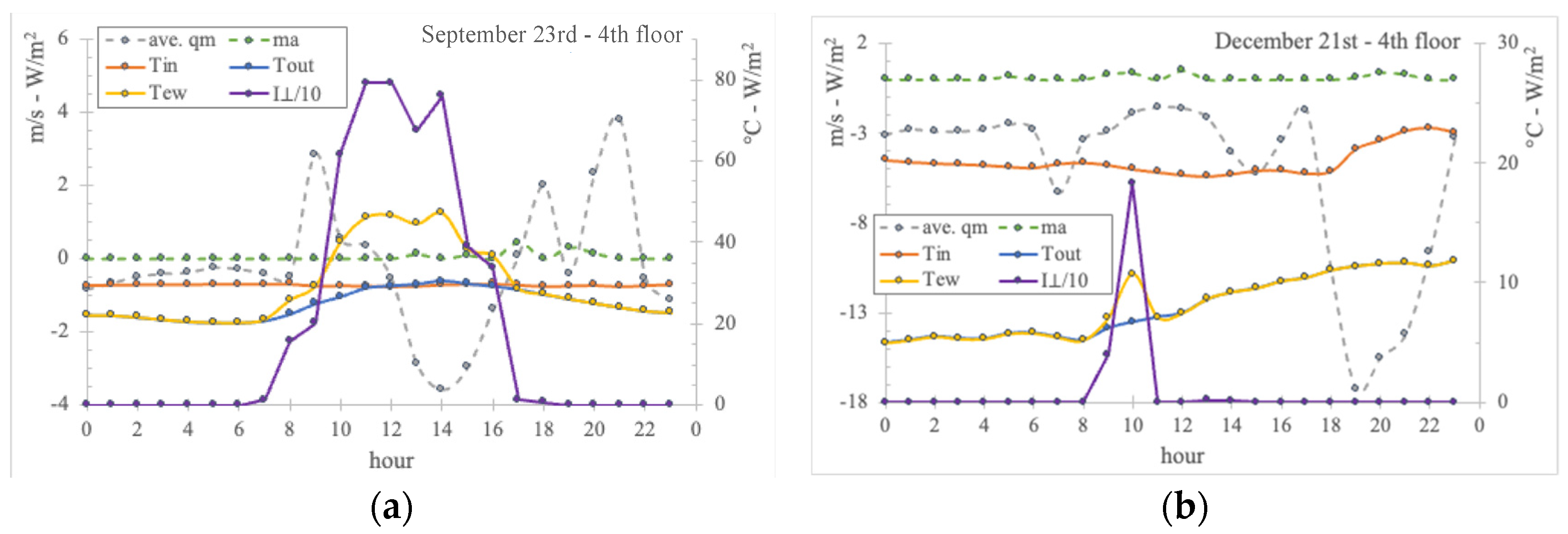
As an example, Figure 1 reports the measured thermal flux hourly for two reference days in the 4th-floor apartment: the differences among the sensors’ outputs are attributed to a possible local non-uniform behavior of the wall, the local installation process of the tiles, and the overall error of the measuring devices, especially for the close-to-null values where the heat transfer changes direction. According to Equation (17), positive values for the heat flux mean thermal gains through the building’s envelope while negative values correspond to thermal losses towards the external environment. Coherently, in Figure 2, the other main indoor and outdoor parameters are shown for the same days (“ave. q_m” is the mean value of thermal flux).

For greater clarity, the graph does not display bands related to the accuracy of the parameters, but these values were considered in the definition of N_i. Based on the instrumentation set-up, relative errors are fixed at around 4% for N₁; 2% for N₂; 2% for N₃; null for N₄, which is related to the assumption of geometry and material properties; 4% for N₅; 2% for N₆; and 5.5% for $N_1^{*}$. In

Table 1. Values of the numbers derived by the π theorem.

${\mathit{N}}_{\mathbf{1}}^{\mathbf{*}}$	${\mathit{N}}_{\mathbf{1}}$	${\mathit{N}}_{\mathbf{2}}$	${\mathit{N}}_{\mathbf{3}}$	${\mathit{N}}_{\mathbf{4}}$	${\mathit{N}}_{\mathbf{5}}$	${\mathit{N}}_{\mathbf{6}}$	${\mathit{N}}_{\mathbf{1}}^{\mathbf{*}}$	${\mathit{N}}_{\mathbf{1}}$	${\mathit{N}}_{\mathbf{2}}$	${\mathit{N}}_{\mathbf{3}}$	${\mathit{N}}_{\mathbf{4}}$	${\mathit{N}}_{\mathbf{5}}$	${\mathit{N}}_{\mathbf{6}}$
5.9 × 10−5	2.0	8.4 × 102	4.2 × 104	0.48	1.39 × 10−1	1.5	9.9 × 10−5	2.0	8.4 × 102	4.2 × 104	0.47	1.39 × 10−1	1.2
1.5 × 10−4	2.1	5.8 × 102	2.8 × 104	0.47	7.70 × 10−1	1.5	1.5 × 10−4	2.1	5.7 × 102	2.8 × 104	0.47	7.70 × 10−1	1.3
3.5 × 10−4	2.1	2.0 × 102	1.1 × 104	0.47	3.35	2.0	5.6 × 10−4	2.1	2.0 × 102	1.1 × 104	0.47	3.35	1.7
1.3 × 10−4	2.1	6.8 × 102	3.8 × 104	0.47	3.85	2.1	1.6 × 10−4	2.1	6.8 × 102	3.8 × 104	0.47	3.85	1.9
2.0 × 10−4	0.1	4.5 × 102	2.2 × 104	0.47	1.59 × 10−3	0.6	2.1 × 10−4	0.4	4.5 × 102	2.2 × 104	0.47	1.59 × 10−3	0.5
8.6 × 10−5	0.4	8.6 × 102	4.8 × 104	0.47	2.08 × 10−3	0.8	5.6 × 10−5	0.2	8.6 × 102	4.8 × 104	0.47	2.08 × 10−3	0.7
8.6 × 10−5	2.1	8.2 × 102	4.8 × 104	0.47	3.84	2.8	7.1 × 10−5	2.1	8.2 × 102	4.8 × 104	0.47	3.84	2.4
5.1 × 10−4	2.0	2.9 × 102	1.0 × 104	0.48	2.68	0.7	1.8 × 10−4	2.1	2.9 × 102	1.0 × 104	0.48	2.68	0.5
7.8 × 10−4	2.0	2.1 × 102	6.9 × 103	0.48	2.32	0.6	1.7 × 10−4	2.1	2.1 × 102	6.9 × 103	0.48	2.32	0.4
3.7 × 10−4	1.9	1.4 × 104	7.2 × 104	0.48	2.64 × 10−2	0.1	8.3 × 10−5	2.3	1.4 × 104	7.2 × 104	0.48	2.64 × 10−2	0.0
4.7 × 10−4	2.0	1.3 × 103	2.3 × 104	0.48	8.59 × 10−1	0.3	1.1 × 10−4	2.0	1.3 × 103	2.3 × 104	0.48	8.59 × 10−1	0.2
7.8 × 10−5	1.6	9.6 × 103	1.7 × 105	0.48	8.20 × 10−3	0.2	7.2 × 10−6	1.0	9.5 × 103	1.7 × 105	0.48	8.20 × 10−3	0.1
4.0 × 10−4	1.8	3.4 × 103	5.3 × 104	0.48	1.90 × 10−2	0.2	2.0 × 10−4	1.3	3.4 × 103	5.3 × 104	0.48	1.90 × 10−2	0.1
1.3 × 10−4	0.4	2.0 × 104	2.1 × 105	0.48	2.05 × 10−3	0.1	7.7 × 10−4	87.7	2.0 × 104	2.1 × 105	0.48	2.05 × 10−3	0.0
1.8 × 10−4	8.9	2.5 × 104	2.1 × 105	0.48	3.13 × 10−4	0.1	3.7 × 10−5	33.7	2.5 × 104	2.1 × 105	0.48	3.13 × 10−4	0.0
2.3 × 10−4	7.3	2.2 × 104	1.7 × 105	0.48	3.65 × 10−4	0.1	1.1 × 10−4	24.7	2.2 × 104	1.7 × 105	0.48	3.65 × 10−4	0.0
2.2 × 10−4	3.5	1.6 × 104	1.3 × 105	0.48	6.15 × 10−4	0.1	4.0 × 10−4	22.6	1.6 × 104	1.3 × 105	0.48	6.15 × 10−4	0.0
7.8 × 10−4	0.0	6.9 × 103	4.1 × 104	0.49	1.71 × 10−3	0.1	1.2 × 10−3	5.5	6.9 × 103	4.1 × 104	0.48	1.71 × 10−3	0.0
6.8 × 10−4	1.5	9.5 × 103	4.8 × 104	0.49	6.82 × 10−3	0.1	1.0 × 10−3	2.8	9.5 × 103	4.8 × 104	0.48	6.82 × 10−3	0.0
7.5 × 10−4	0.1	3.7 × 103	3.5 × 104	0.48	1.59 × 10−3	0.1	1.2 × 10−2	61.5	3.7 × 103	3.5 × 104	0.48	1.59 × 10−3	0.0
2.9 × 10−4	1.4	3.0 × 103	4.4 × 104	0.48	5.79 × 10−3	0.2	4.0 × 10−4	0.7	3.0 × 103	4.4 × 104	0.48	5.79 × 10−3	0.1
1.2 × 10−4	13.6	1.2 × 104	1.0 × 105	0.50	2.94 × 10−4	0.0	4.2 × 10−5	6.4	1.2 × 104	1.0 × 105	0.50	2.94 × 10−4	0.1
1.5 × 10−4	18.6	1.3 × 104	1.1 × 105	0.50	2.05 × 10−4	0.0	3.7 × 10−5	7.9	1.3 × 104	1.1 × 105	0.50	2.05 × 10−4	0.1
2.7 × 10−5	21.4	1.7 × 104	1.2 × 105	0.50	1.75 × 10−4	0.0	3.6 × 10−5	8.4	1.7 × 104	1.2 × 105	0.50	1.75 × 10−4	0.1
9.2 × 10−5	105.0	1.3 × 105	1.3 × 105	0.50	3.31 × 10−5	0.0	5.4 × 10−5	9.1	1.3 × 105	1.3 × 105	0.50	3.31 × 10−5	0.1
6.6 × 10−5	7.0	1.2 × 104	9.2 × 104	0.50	3.78 × 10−4	0.1	2.5 × 10−4	12.8	1.2 × 104	9.3 × 104	0.49	3.78 × 10−4	0.0
4.5 × 10−5	4.9	3.7 × 103	4.4 × 104	0.50	4.95 × 10−4	0.1	3.2 × 10−3	67.3	3.7 × 103	4.4 × 104	0.49	4.95 × 10−4	0.0
5.1 × 10−3	56.9	8.4 × 103	1.8 × 104	0.50	6.21 × 10−5	0.0	2.4 × 10−3	16.8	8.4 × 103	1.8 × 104	0.50	6.21 × 10−5	0.0
2.8 × 10−1	1311.4	2.7 × 105	1.4 × 104	0.50	2.60 × 10−6	0.0	4.7 × 10−3	18.5	2.7 × 105	1.4 × 104	0.50	2.60 × 10−6	0.0
2.0 × 10−5	1.5	1.5 × 104	7.0 × 104	0.50	7.30 × 10−3	0.0	6.8 × 10−4	0.2	1.5 × 104	7.0 × 104	0.50	7.30 × 10−3	0.0
7.3 × 10−5	1.9	9.1 × 102	5.2 × 104	0.47	2.60 × 10−2	1.9	9.0 × 10−5	1.9	9.1 × 102	5.2 × 104	0.47	2.60 × 10−2	1.5
4.2 × 10−5	1.4	1.1 × 103	6.1 × 104	0.47	5.28 × 10−3	1.2	7.7 × 10−5	1.2	1.1 × 103	6.1 × 104	0.47	5.28 × 10−3	0.9

the full matrix is displayed with the complete dataset from the 3rd and the 4th floor.

2.3. Regression Analysis

The values of the matrix already mentioned have been systematized through VB coding within Excel™ 2021 in order to approximate the 7 missing coefficients of the equation derived from the π theorem (a, b, c, d, e, f, and g). Matlab™ 2021a has also been utilized as a verification tool for the same results.

In general, the overall quality of a regression can be assessed by examining the coefficient of determination R² (in the simple and adjusted form) and the standard error (SE). The first one represents the correlation between the parameters obtained from measurement data and the values predicted by the model function; hence, its value will always fall within 0 and 1. In

Table 2. The main regression parameters.

	Degrees of Freedom (DF)	Sum of Squares (SS)	Mean Square (MS)
Regression	$DFM=p$	$SSM=\sum {\left(\widehat{y_i}-\overline{y}\right)}^2$	SSM/DFM = MSM
Residual (Error)	$DFE=n-p-1$	$SSE=\sum {\left(y_i-\widehat{y_i}\right)}^2$	SSE/DFE = MSE
Total	$DFT=n-1$	$SST=\sum {\left( y_i-\overline{y}\right)}^2$	SST/DFT

With: p number of variables; n number of equations; $\widehat{y_i}$ predicted value from the model; $\overline{y}$ mean value of the observations; and $y_i$ i-th observed value.

, the equations and reference nomenclature are provided.

Consequently, the determination coefficient results:

$$R^2=\frac{SSM}{SST}$$

(18)

The need to correct the standard R² arises because it tends to become higher as the number of variables considered for the model increases, even if such variables have a weak influence on the predicted function. The adjusted form $R_{adj}^2$ is thus defined as follows, taking into account the number of variables in the model (it will be always minor than R²):

$$R_{adj}^2=1-\left[\left(1-R^2\right) \left(\frac{n-1}{n-p-1}\right)\right]=1-\left[\left(1-R^2\right)\left(\frac{DFT}{DFE}\right)\right]$$

(19)

3. Results

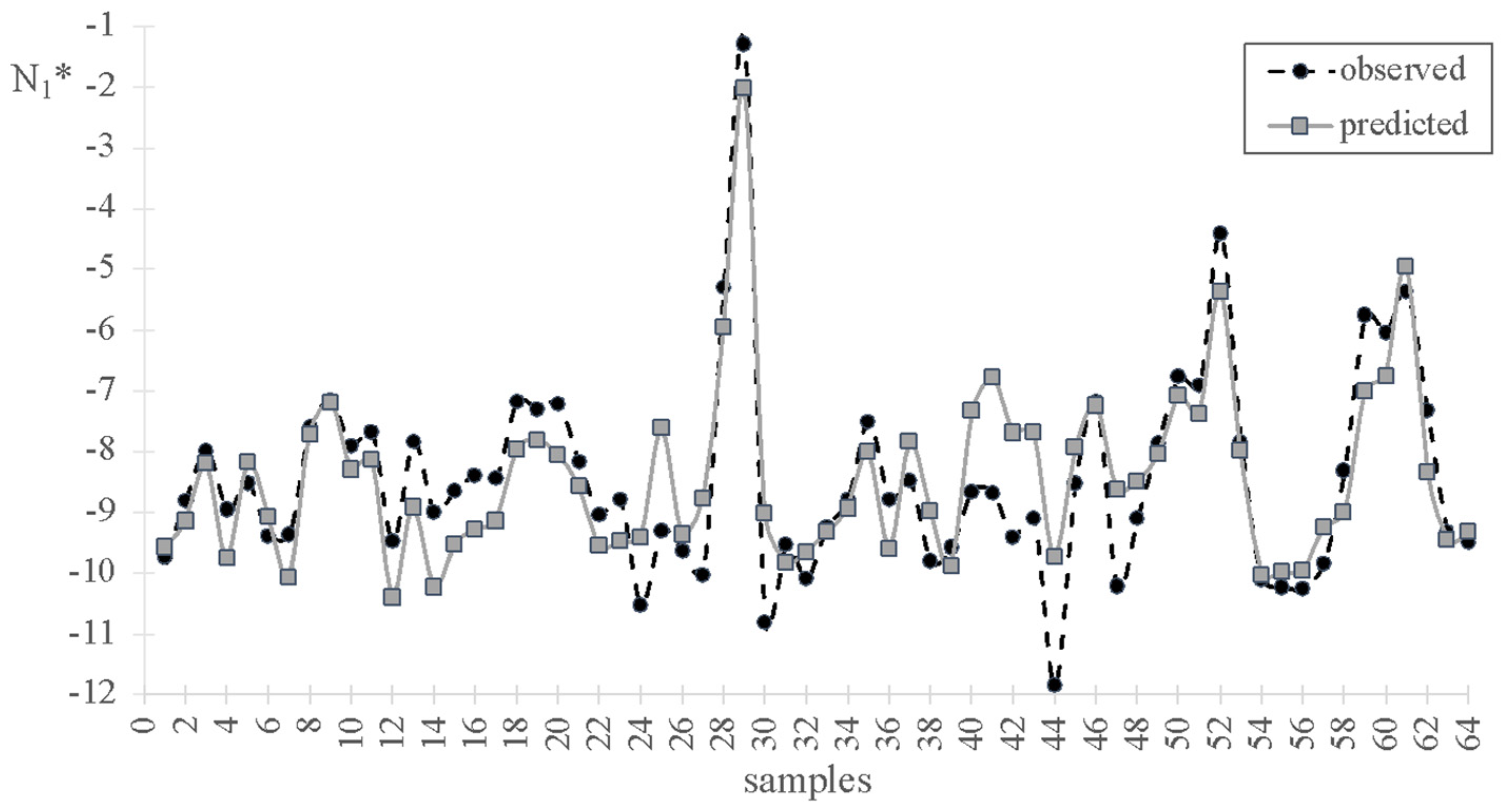
The correlation algorithm has led to the extrapolation of the coefficients of the requested equation, which are presented in

Table 3. Coefficients for the obtained correlation and statistical parameters.

Coefficients		Regression Statistics
a	8.4 × 10−12	$R^2$	0.74
b	0.081	$R_{adj}^2$	0.71
c	0.28	RSE	0.89
d	−1.52	observations	64
e	−40.7
f	−0.052
g	−0.6

. The regression statistics indicate a good relationship among the parameters identified through the analysis of the Buckingham theorem, with a coefficient of determination greater than 70%, even in the adjusted form and absolute standard error equal to 0.89. A qualitative comparison between the parameter derived from experimental data and predicted by regression is shown in Figure 3. The relative mean residual value for the 64 samples achieves 8.1%.

In other words, it can be asserted that the equation and the parameters derived from the Buckingham theorem, together with the coefficients obtained from the approximation of the available experimental dataset, describe satisfactorily the relation among the energy performance of an opaque wall (in the form of thermal loss) and the internal (due to users) and external loads (weather conditions and radiation).

4. Conclusions

The Buckingham π theorem has been used in the context of building physics to consider the main parameters responsible for heat transfer and thermal loss, deriving the behavior of a separation wall set between the internal and external environment.

Some proper dimensionless coefficients summarized the main occurrent phenomena such as the variable presence of wind, solar radiation, and the daily natural oscillation of temperatures, linking them to each other. The method is robust in its physical/mathematical formulation, and the correlation was validated thanks to the presence of numerous experimental data obtained within a real context. The results of the regression statistics show an effectual correlation among the numbers identified through the Buckingham theorem, with a coefficient of determination greater than 70%.

There are many interesting aspects of the test campaign, upstream of this research, that give strength to the extrapolation of the dimensional analysis. First, the two flats are inhabited, and they are distinct (the one on the 3rd floor and the other one on the 4th, so the habits of different users are observed), but the walls under investigation are similar and completely homogeneous in the stratigraphy of the materials (no windows or cross-section cut). They are also exposed to the same orientation and external conditions during the year (air temperature and solar radiation). The thermal flux is not derived from other parameters (design-based values for thermal transmittance of walls and temperatures are indeed not suitable in very dynamic operative conditions without strong post-processing algorithms), but it is directly monitored through the specific tile sensor [3]. Therefore, the output voltage is linear with the specific power [W/m²] in the range of interest. Accordingly, the thermal power in real time and the integrated energy during the whole season [kWh/m²] reflect the actual interactions among the building envelope, the energy systems operation, and the behavior of occupants, with respect to the external boundary conditions identifying the energy performance of the wall.

Once the correlation is validated and the coefficients found, the approach of dimensionless analysis is flexible and can be extended to different contexts to compile estimates of energy performance and then the sustainability of other structures such as blocks, mapping their positions, orientations, and main materials without resorting to complex, invasive, and time-consuming experimental campaigns.

References

- Official Journal of the European Union. European Union Directive (EU) 2018/844 of the European Parliament and of the Council of 30 May 2018 Amending Directive 2010/31/EU on the Energy Performance of Buildings and Directive 2012/27/EU on Energy Efficiency; Official Journal of the European Union: Luxembourg, 2018. [Google Scholar]
- Tarpani, E.; Piselli, C.; Fabiani, C.; Pigliautile, I.; Kingma, E.J.; Pioppi, B.; Pisello, A.L. Energy Communities Implementation in the European Union: Case Studies from Pioneer and Laggard Countries. Sustainability 2022, 14, 12528. [Google Scholar] [CrossRef]
- Pierucci, G.; Balocco, C.; de Lucia, M. Development of a New Heat Flux Sensor for Building Applications. Int. J. Heat Technol. 2020, 38, 794–800. [Google Scholar] [CrossRef]
- Diller, T.E. Advances in Heat Flux Measurements. In Advances in Heat Transfer; Elsevier: Amsterdam, The Netherlands, 1993; Volume 23, ISBN 0120200236. [Google Scholar]
- Childs, P.R.N.; Greenwood, J.R.; Long, C.A. Heat Flux Measurement Techniques. Proc. Inst. Mech. Eng. Part C J. Mech. Eng. Sci. 1999, 213, 655–677. [Google Scholar] [CrossRef]
- Yüksel, N. Methods and Techniques for Measuring the Thermal Conductivity of Insulation Materials. In Insulation Materials in Context of Sustainability; Almusaed, A., Almssad, A., Eds.; Intech Open Science: London, UK, 2016; pp. 115–123. [Google Scholar]
- Flanders, S.N. Heat Flux Transducers Measure In-Situ Building Thermal Performance. J. Therm. Insul. Build. Envel. 1994, 18, 28–52. [Google Scholar] [CrossRef]
- Zarr, R.R.; Martínez-Fuentes, V.; Filliben, J.J.; Dougherty, B.P. Calibration of Thin Heat Flux Sensors for Building Applications Using ASTM C 1130. J. Test. Eval. 2011, 29, 293–300. [Google Scholar] [CrossRef]
- ASTM International C177-97; Standard Test Method for Steady-State Heat Flux Measurements and Thermal Transmission Properties by Means of the Guarded-Hot-Plate Apparatus. ASTM International: West Conshohocken, PA, USA, 2004.
- ASTM International C518-15; Standard Test Method for Steady-State Thermal Transmission Properties by Means of the Heat Flow Meter Apparatus. ASTM International: West Conshohocken, PA, USA, 2015.
- Pullins, C.A.; Diller, T.E. In Situ High Temperature Heat Flux Sensor Calibration. Int. J. Heat Mass Transf. 2010, 53, 3429–3438. [Google Scholar] [CrossRef]
- Zhang, C.; Huang, J.; Li, J.; Yang, S.; Ding, G.; Dong, W. Design, Fabrication and Characterization of High Temperature Thin Film Heat Flux Sensors. Microelectron. Eng. 2019, 217, 111128. [Google Scholar] [CrossRef]
- Langley, L.W.; Barnes, A.; Matijasevic, G.; Gandhi, P. High-Sensitivity, Surface-Attached Heat Flux Sensors. Microelectron. J. 1999, 30, 1163–1168. [Google Scholar] [CrossRef]
- Gidik, H.; Bedek, G.; Dupont, D.; Codau, C. Impact of the Textile Substrate on the Heat Transfer of a Textile Heat Flux Sensor. Sens. Actuators A Phys. 2015, 230, 25–32. [Google Scholar] [CrossRef]
- Saidi, A.; Kim, J. Heat Flux Sensor with Minimal Impact on Boundary Conditions. Exp. Therm. Fluid Sci. 2004, 28, 903–908. [Google Scholar] [CrossRef]
- Cucumo, M.; Ferraro, V.; Kaliakatsos, D.; Mele, M. On the Distortion of Thermal Flux and of Surface Temperature Induced by Heat Flux Sensors Positioned on the Inner Surface of Buildings. Energy Build. 2018, 158, 677–683. [Google Scholar] [CrossRef]
- Biddulph, P.; Gori, V.; Elwell, C.A.; Scott, C.; Rye, C.; Lowe, R.; Oreszczyn, T. Inferring the Thermal Resistance and Effective Thermal Mass of a Wall Using Frequent Temperature and Heat Flux Measurements. Energy Build. 2014, 78, 10–16. [Google Scholar] [CrossRef]
- ISO 9869-1:2014; Thermal Insulation—Building Elements—In-Situ Measurement of Thermal Resistance and Thermal Transmittance—Part 1: Heat Flow Meter Method. ISO: Geneva, Switzerland, 2014.
- Rasooli, A.; Itard, L. In-Situ Characterization of Walls’ Thermal Resistance: An Extension to the ISO 9869 Standard Method. Energy Build. 2018, 179, 374–383. [Google Scholar] [CrossRef]
- Distefano, D.L.; Gagliano, A.; Naboni, E.; Sapienza, V.; Timpanaro, N. Thermophysical Characterization of a Cardboard Emergency Kit-House. Math. Model. Eng. Probl. 2018, 5, 168–174. [Google Scholar] [CrossRef]
- Baccilieri, F.; Bornino, R.; Fotia, A.; Marino, C.; Nucara, A.; Pietrafesa, M. Experimental Measurements of the Thermal Conductivity of Insulant Elements Made of Natural Materials: Preliminary Results. Int. J. Heat Technol. 2016, 34, S413–S419. [Google Scholar] [CrossRef]
- Cardinale, T.; Arleo, G.; Bernardo, F.; Feo, A.; De Fazio, P. Investigations on Thermal and Mechanical Properties of Cement Mortar with Reed and Straw Fibers. Int. J. Heat Technol. 2017, 35, S375–S382. [Google Scholar] [CrossRef]
- Cardinale, T.; Sposato, C.; Alba, M.; Feo, A.; Grandizio, F.; Lista, G.; Montesano, G.; Fazio, P. Energy and Mechanical Characterization of Composite Materials for Building with Recycled PVC. Tec. Ital. J. Eng. Sci. 2019, 63, 129–135. [Google Scholar] [CrossRef]
- Cesaratto, P.G.; De Carli, M. A Measuring Campaign of Thermal Conductance in Situ and Possible Impacts on Net Energy Demand in Buildings. Energy Build. 2013, 59, 29–36. [Google Scholar] [CrossRef]
- Langhaar, H.L. Dimensional Analysis and Theory of Models; Wiley: New York, NY, USA, 1951. [Google Scholar]
- Balocco, C. A Non-Dimensional Analysis of a Ventilated Double Façade Energy Performance. Energy Build. 2004, 36, 35–40. [Google Scholar] [CrossRef]
- Wang, R.J.; Pan, Y.H.; Cheng, W.L. A Dimensionless Study on Thermal Control of Positive Temperature Coefficient (PTC) Materials. Int. Commun. Heat Mass Transf. 2021, 120, 104987. [Google Scholar] [CrossRef]
- Trethowen, H. Measurement Errors with Surface-Mounted Heat Flux Sensors. Build. Environ. 1986, 21, 41–56. [Google Scholar] [CrossRef]
- Curtis, W.D.; Logan, J.D.; Parker, W.A. Dimensional Analysis and the Pi Theorem. Linear Algebra Appl. 1982, 47, 117–126. [Google Scholar] [CrossRef]
- Balocco, C.; Pierucci, G.; De Lucia, M. An Experimental Method for Building Energy Need Evaluation at Real Operative Conditions. A Case Study Validation. Energy Build. 2022, 266, 112114. [Google Scholar] [CrossRef]
- Zhang, Z.; Yao, J.; Zheng, R.; Berardi, U.; Santos, P.; Zhang, Z.; Yao, J.; Zheng, R. Multi-Objective Optimization of Building Energy Saving Based on the Randomness of Energy-Related Occupant Behavior. Sustainability 2024, 16, 1935. [Google Scholar] [CrossRef]
- Natarajan, Y.; K. R., S.P.; Wadhwa, G.; Choi, Y.; Chen, Z.; Lee, D.-E.; Mi, Y. Enhancing Building Energy Efficiency with IoT-Driven Hybrid Deep Learning Models for Accurate Energy Consumption Prediction. Sustainability 2024, 16, 1925. [Google Scholar] [CrossRef]
- Buckingham, E. On Physically Similar Systems; Illustrations of the Use of Dimensional Equations. Phys. Rev. 1914, 4, 345–376. [Google Scholar] [CrossRef]
- Comune di Firenze EX LONGINOTTI—Edificio Sperimentale in Legno per 40 Alloggi e.r.P. Available online: https://www.casaspa.it/data/archive/informazioni/stendardi_exlonginotti.pdf (accessed on 1 March 2024).
- UNI/TS 11300-1:2014; Prestazioni Energetiche Degli Edifici—Parte 1: Determinazione del Fabbisogno di Energia Termica Dell’edificio per la Climatizzazione Estiva ed Invernale. UNI: Milano, Italy, 2014.
- Singh, S.; Yadav, M.; Khandekar, S. Measurement issues associated with surface mounting of thermopile heat flux sensors. Appl. Therm. Eng. 2017, 114, 1105–1113. [Google Scholar] [CrossRef]
- Wright, R.E.; Kantsios, A.G.; Henley, W.C. Effect of Mounting on the Performance of Surface Heat Flow Meters Used to Evaluate Building Heat Losses. In Thermal Insulation, Materials, and Systems for Energy Conservation in the’80s; ASTM International: West Conshohocken, PA, USA, 1983; Volume 789, pp. 293–317. [Google Scholar] [CrossRef]
- Consorzio LaMMA. Available online: https://www.lamma.toscana.it/ (accessed on 1 March 2024).
- Gatley, D.P. Understanding Psychrometrics; EBSCO ebook academic collection; ASHRAE: Atlanta, GA, USA, 2013; ISBN 9781936504312. [Google Scholar]
Figure 1.
Hourly trend for the heat flux passing through the measured wall on the 4th floor (a) on September 23rd and (b) on December 21st.
Figure 2.
Hourly trend curve for some of the main indoor and outdoor monitored parameters (a) on September 23rd and (b) on December 21st.
Figure 3.
Values of according to experimental data and predicted by regression.