

Prediction of Losses Due to Dust in PV Using Hybrid LSTM-KNN Algorithm: The Case of Saruhanlı

Department of Electronic and Automation, Vocational School, Batman University, Batman 72100, Turkey
Sustainability 2024, 16(9), 3581; https://doi.org/10.3390/su16093581
Submission received: 22 December 2023
/
Revised: 1 April 2024
/
Accepted: 16 April 2024
/
Published: 24 April 2024
Abstract
:Sustainable and renewable energy sources are of great importance in today’s world. In this respect, renewable energy sources are used in many fields of technology. In order to minimize dust on PV panels and ensure their sustainability, power losses due to dust must be estimated accurately. In this way, the efficiency of a sustainable energy source will increase and serious economic savings can be achieved. In this study, a hybrid deep learning model was designed to predict losses caused by dust in PV panels installed in the Manisa Saruhanlı district. The hybrid deep learning model consists of Long Short-Term Memory (LSTM) and K-Nearest-Neighbors (KNN) algorithms. The performance of the proposed hybrid deep learning model was compared with LSTM and KNN algorithms. Sensitivity analysis was performed to statistically evaluate the prediction results. The input variables of the models were time, sunshine duration, humidity, ambient temperature and solar radiation. The output variable was the losses caused by dust in the PV panels. Hybrid LSTM-KNN, LSTM and KNN models predicted losses caused by dust in PV panels with 98.22%, 95.51% and 61.49% accuracy. The hybrid LSTM-KNN model predicted losses caused by dust in PV panels with higher accuracy than other models. Using LSTM and KNN algorithms together improved the performance of the hybrid deep learning model. With sensitivity analysis, it was found that solar radiation is the most important variable affecting the losses caused by dust in PV panels.
1. Introduction
With technological and economic advancements, humankind’s need for energy has increased. Due to many negative reasons, such as air pollution, the depletion of fossil fuels, global warming, climate change and acid rain, renewable energy is preferred instead of traditional energy. Solar energy is a promising type of energy in the field of renewable energy [1]. Solar energy converts the energy coming from the sun directly into electrical energy. Solar energy is widely used in many areas such as cooking, vehicle charging, and home heating [2]. Photovoltaic (PV) panels are widely used all over the world due to their advantages such as low operating costs, zero emissions, minimum maintenance and high power density. The efficiency of PV modules depends on climatic parameters such as accumulated dust, relative humidity, temperature, wind speed and solar radiation [3]. Uneven dust accumulation on PV panels leads to losses in transmission. In addition, it shortens the lifetime of PV panels and the lifetime of the equipment [4]. Dust particles accumulated on the surface of the PV modules cause scattering and reflection of the incoming solar radiation and thus impair the solar energy production efficiency [5]. The shape and size of the dust particles affecting the light transmittance of PV panels are important. Particles with a diameter of 0.05 mm are considered small particles, particles with a diameter between 0.05 and 2 mm are considered medium particles and particles with a diameter between 2 and 57 mm are considered large particles. Small particles accumulated on the PV cause loss of radiation. Small particles have a greater impact on performance compared to large particles. Dust particles in agricultural areas consist of soil, organic pollen and bird droppings. In urban areas, dust particles come from exhaust gases. In coastal areas, on the other hand, it is the result of the accumulation of salt [6]. Air pollution causes a 6.4% reduction in the efficiency of PV panels. On the other hand, dust causes a 40% reduction in the efficiency of PV panels [7]. Examining the effects of dust losses on photovoltaic modules is important in calculating the efficiency of PV panels. In addition, an accurate estimation of dust losses of PV panels is important for maintenance and repair [8].
Kouz et al. [9] used artificial neural network (ANN) and extreme learning machine (ELM) algorithms to estimate energy losses due to dust and ambient temperatures. The prediction accuracies of the ELM model and ANN model are 91.42% and 90.69%, respectively. Hammad et al. [10] used Multivariate Linear Regression (MLR) and ANN models to calculate the energy losses and economic losses of PV panels due to dust. The MLR and ANN models predicted the energy and cost losses due to dust at 87.7% and 90%, respectively. Adıgüzel et al. [11] used an Adaptive Neuro-Fuzzy Inference System (ANFIS) to forecast the performance of photovoltaic modules exposed to dust. The ANFIS Algorithm Root mean square error (RMSE) = 0.18719 and the coefficient of determination for monocrystalline silicon PV modules and the RMSE = 0.87098 and for polycrystalline PV modules. Javed et al. [12] used the ANN and MLR models to forecast the performance loss of PV panels in Qatar due to dust. While the ANN model is and the mean squared error (MSE) = 0.0038, the MLR model is and MSE = 0.0082. The ANN model showed better performance compared to the MLR model. Perez et al. [13] used ANN to estimate losses resulting from dust. With new technology, ANN is successful in predicting losses and its performance metrics are normalized root mean square errors (NRMSE) = 6.79 and R = 0.91. Zitouni et al. [14] used the MLR, Interactive Multivariate Linear Regression Model (MLRWI), Response Surface Methodology (RSM) and the ANN to predict the loss due to dust in PV panels. The ANN produced better prediction results than the other models. and RMSE are 0.813 and 0.026, respectively. Jamil et al. [15] used the ANN, recurrent neural network (RNN) and hybrid convolutional neural network (CNN)-LSTM algorithm to estimate performance ratio and soiling loss in PV panels. The performance error values of the hybrid CNN-LSTM algorithm are RMSE, mean absolute error (MAE), mean absolute percentage error (MAPE) and mean bias error (MBE) at 0.00385, 0.04358, 0.28478 and 0.00217, respectively. The hybrid CNN-LSTM algorithm predicted better than other algorithms. Pavan et al. [16] developed four Bayesian Neural Networks (BNN) to predict losses due to dust. The performance indexes of the proposed BNN model are R, RMSE, MAE and MAPE, at 99.96%, 0.22, 0.08 and 2.3, respectively. Valasquez and Ezcurra [17] used a random forest model to estimate production loss due to dust. The MAE, mean square error (MSE) and of the proposed algorithm are 0.22, 0.07 and 0.88, respectively.
We can list this study’s contributions to the world of science in terms of contextualization as follows:
- -
- The hybrid LSTM-KNN algorithm has not been used in the literature to estimate losses due to dust in PV panels.
- -
- The hybrid LSTM-KNN algorithm was used to improve the performance of LSTM and KNN algorithms. A better prediction was achieved with the hybrid LSTM-KNN algorithm than with the LSTM and KNN algorithm. However, the prediction time of the hybrid LSTM-KNN algorithm was longer than that of the LSTM and KNN algorithms.
- -
- Hybrid LSTM-KNN, LSTM and KNN algorithms were implemented in the same simulation and with the same data. Since algorithms use random values in the different simulations, different data sets may occur. This may cause comparison results to be inaccurate.
- -
- Dust loss in PV panels is affected by meteorological data. In this context, the most important factor affecting dust loss in PV panels was determined to be solar radiation. This is a factor that increases the efficiency of the solar panel during the installation phase.
- -
- The power losses of PV panels due to dust were calculated using different algorithms in the literature. In this context, Pavan et. al. predicted 99.92% of the power loss due to dust using the BNN model. This estimate is the best performance in the literature. In this study, the Hybrid LSTM-KNN algorithm predicted 98.22% of the loss due to dust in PV panels. In this respect, a better result was obtained in this study than many other studies in the literature.
- -
- In our previous studies, the dust loss of PV panels was estimated with hybrid LSTM-SVM, hybrid LSTM-tree, and hybrid LSTM-ensemble. However, the results obtained from other hybrid algorithms were below the values obtained from the hybrid algorithm used in this study.
- -
- Among the algorithms that estimate the power losses of PV panels due to dust, the hybrid algorithm has not been used much in the literature. Therefore, a hybrid algorithm was used in this study.
2. Materials and Methods
2.1. Data
The Saruhanlı district of Manisa is situated in the Aegean Region in Turkey and is a flat and fertile land in the Gediz Lowland. With a surface area of 842 km2, this district is 43 m above sea level. In the south of the district, there are Turgutlu and Ahmetli; in the northeast and east, Akhisar and Gölmarmara; in the southwest, Manisa and in the northwest, Kırık [18]. In Saruhanlı, it is cold and rainy in winter and hot and dry in summer. The highest rainfall in the Saruhanlı District is 86 millimetres on average, while the lowest rainfall is 3 millimetres. The highest temperature is 35 °C in July and the lowest temperature is 2 °C in January [19]. In Figure 1, you can see a satellite view of the Saruhanlı District.
In this study, production data from PV panels were taken from the switchgear facility established in the Saruhanlı district of Manisa. In this region, solar panels are organized according to different solar angles. As shown in Figure 2, solar power plants are installed in two different regions in this facility. The solar power plant in the 1st region is called GES1, while the solar power plant in the 2nd region is called GES2; a total of 13,716 kWp of electrical energy is generated. The solar panels in the GES1 region are identified as SEM1, SEM3, SEM4, SEM5, SEM6, SEM7 and SEM8 and the solar panels in the GES2 region are identified as SEM1, SEM3, SEM4, SEM5 and SEM6. The data in this study were taken from the SEM4 solar power plant in the GES1 region.
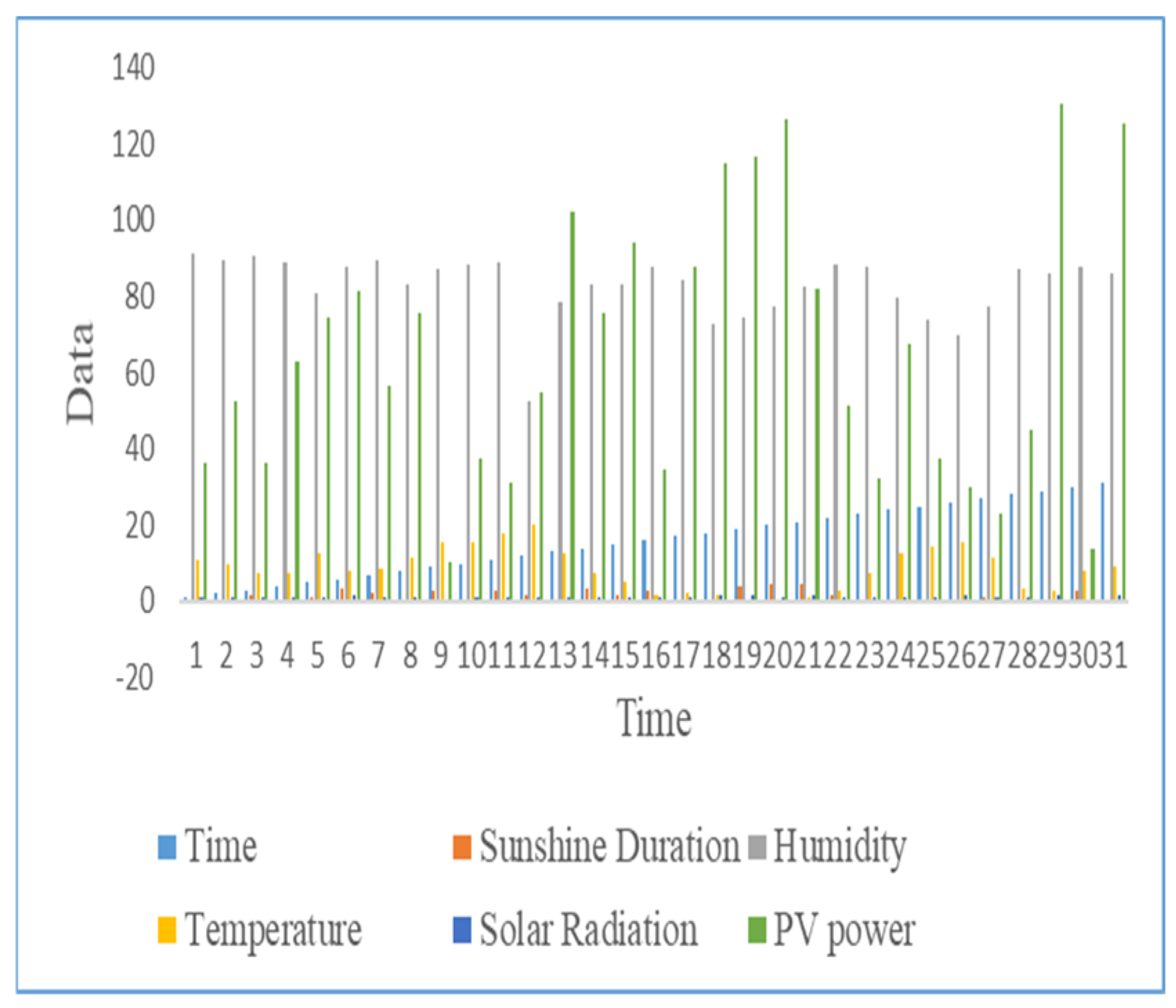
In this study, one year of daily data from the PV power plant was used. However, Table 1 presents the daily data of the PV power plant for January. Figure 3 shows the input and output data of the solar power plant for January. This plant consists of 33 inverters and 6 strings. The SEM4 power plant consists of 4356 solar panels and generates 1176. 12 kWp DC electrical energy. Input data and output data for January are presented in Figure 3. Sunshine duration, humidity, wind speed, temperature and solar radiation data were taken from the General Directorate of Meteorology, Ministry of Environment, Urbanization and Climate Change of the Republic of Turkey.
2.2. Sensitivity Analysis
In this study, the cosine amplitude method (CAM) was used to analyze the relationship between the input and output data of the Hybrid LSTM-KNN algorithm. A data series was created by collecting data samples as shown in Equation (1) [23].
The data array is a vector consisting of data. m represents the length of the vector.
The data represent a point in m-dimensional space. A coordinate is required to describe these points. represents the relationship between data sample and data sample .
Equation (3) shows that the cosine function is related to the dot product. If two vectors are at right angles, their inner product is zero, while if they are collinear, their product is unity [24].
2.3. K-Nearest Neighbor Algorithm
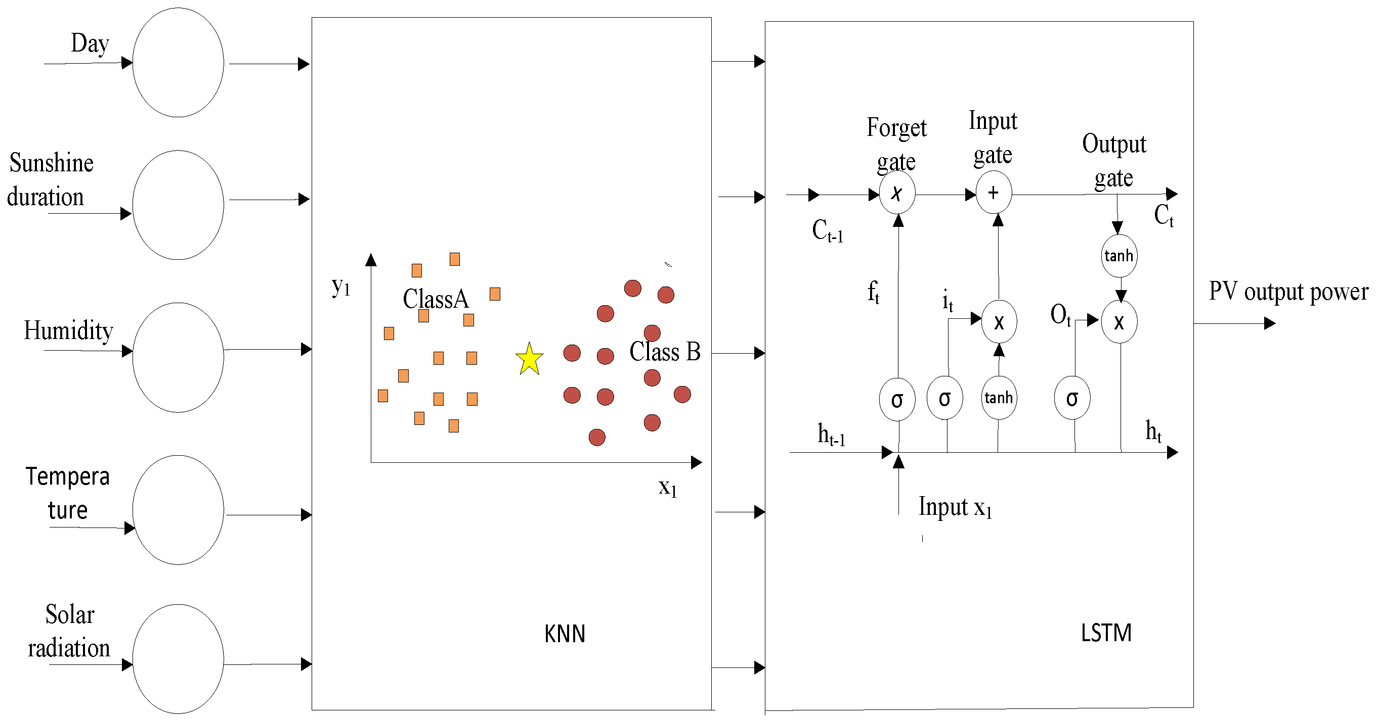
KNN is a method used to predict parametric data that are difficult to predict. KNN can be divided into regression and classification methods. The architecture of the KNN algorithm is presented in Figure 4. When KNN is used as a classifier, it classifies the data by grouping them according to their characteristics. The classification model is used to predict created situations and to predict pre-processed data. The KNN classification method is one of the simplest classification techniques as it consumes less information in data distribution compared to other classification methods. Classification is defined by K selection and Euclidean distance metrics. When KNN is used as a regression, it is used to predict processed data [25]. The KNN algorithm is widely used in many problems such as data mining, fault detection and pattern recognition [26]. KNN selects the most representative and historical datasets instead of all datasets. It allows the estimation of representative samples in problem-solving; therefore, historical data sets can be used effectively. The key features of KNN are as follows:
- Feature Vector: This refers to the current model state and past information. To create a feature vector under the KNN procedure, a trade-off between accuracy and runtime is required.
- Distance Metric: This refers to the Euclidean distance used to measure the distance between a feature vector and a subset of it.
- The number of Nearest Neighbors (K): The datasets are arranged according to their Euclidean distances and K-nearest neighbors are selected. If a higher K value is picked, this leads to data redundancy in prediction, whereas if a lower value is chosen, this leads to a loss of information in historical datasets [27].
In this formula, i refers to the index number and d refers to the Euclidean distance whereas x, y refer to the data points consisting of N dimensions. In the KNN algorithm, when the training data set is huge, it may take a long time to calculate the distance of each training sample. Moreover, it is unclear which distance should be used to obtain the best result [28].
2.4. Long Short-Term Memory
RNN demonstrates the ability to sequentially place multi-layered data. It creates a loop by transferring the data from the input layer to the hidden layer at the very next time step. This cycle improves the ability to learn and abstract by retaining information from the previous cycle. However, in long-term studies, there is a gradient loss when calculating backpropagation. The LSTM is proposed to improve the RNN [29]. The LSTM network can remember previous information for a long time because it uses a non-linear activation function in each layer while addressing large-sized parameters. Therefore, it is widely used in time series problems. The LSTM network architecture is given in Figure 5. The LSTM consists of three gates: forget, input and output. The first layer of the memory gate is the forgotten layer, which ensures that unnecessary information will be forgotten and necessary information will be stored.
is the forgetting threshold at time t, σ is the sigmoid activation function, is the weight, is the input value, is the weight, is the output value and is the bias. The gateway is the second layer and this decides what information should be stored.
While ,, and refer to the weights, and refer to the bias. Equation (8) is used to update the state of a cell at time T.
The output layer is the third layer and is given in Equation (9).
is the output threshold at time t, is the weights, is the input value, is the weight and is the bias term.
is the output value at time t, tanh is the activation function and is the state of the cell at time t.
2.5. Hybrid LSTM-KNN Algorithm
In this study, a hybrid LSTM-KNN algorithm is proposed to estimate losses caused by dust in PV panels. The flow diagram of this algorithm is shown in Figure 6. The inputs of these algorithms include time, sunshine duration, humidity, ambient temperature and solar radiation. The output is the power losses caused by dust in the PV panels. The KNN part of hybrid deep learning pre-processes input data. The iteration is repeated until the optimization process is completed. Then, the data taken from the output of KNN are given to the input of LSTM. The LSTM algorithm splits the optimized data into 90% training data and 10% testing data. The training and testing procedure continues until the end of the iteration. The iteration continues until the training and testing procedure is completed. The error metrics and prediction results of the hybrid LSTM-KNN algorithm are obtained. After the completion of the hybrid algorithm, the KNN algorithm and the LSTM algorithm are run. Right after the hybrid algorithm stops running, the KNN algorithm starts to run. The results of the KNN algorithm are obtained. Once the KNN algorithm is completed, the LSTM algorithm starts to run. The performance indicators of the LSTM algorithm and the prediction results are obtained. A schematic representation of the hybrid deep learning model used in this study is shown in Figure 7.
2.6. Performance Metrics
The performance metrics of the algorithms are , the mean squared error (MSE) RMSE, NRMSE, MAPE MAE and peak signal-to-noise ratio (PSNR). The performance metrics reveal the accuracy of the forecasts made. is shown in Equation (11). The metric shows the relationship between the actual data and predicted data. The value ranges between 1 and 0. The closer the obtained result is to 1, the better the prediction [32,33].
The MSE is shown in Equation (12). The MSE is advantageous when major errors need to be minimized. It is the basis of many statistical methods due to its being differentiable. However, in outliers, the MSE may incorrectly affect the performance of the model. The MAE metric is given in Equation (13). The MAE is less sensitive to outliers. It provides better performance on outliers by attaching the same emphasis to all faults. The RMSE is shown in Equation (14). The RMSE metric is given in Equation (14). The RMSE shows the standard deviation of the errors. If the RMSE is within a limited range with regard to the test and training samples, the model does not overfit [34].
The MAPE metric is given in Equation (15). The MAPE error metric is of particular importance for regression models. It has an intuitive interpretation in terms of relative error. It is used for absolute variances sensitive to relative changes. However, there are some drawbacks to this. Since it is restricted to positive data by definition, this indicates that it is intended for low predictions. It is not suitable for major faults [35].
The NRMSE is shown in Equation (16). The NRMSE is used for a clear reading of the error. It is the ratio of the root mean square of the error to the observed variable. When the NRMSE = 0, this indicates perfect prediction, while NRMSE = 1 indicates statistical prediction. The peak signal-to-noise ratio (PSNR) is given in Equation (17) [36,37].
3. Results and Discussions
3.1. The Sensitivity Analysis of Results
In this study, sensitivity analysis was used to determine the relationship between losses caused by dust in PV panels and experimental variables. Sunbathing, humidity, temperature and solar radiation were used as experimental variables. The sensitivity analysis results are shown in Figure 8. As seen in Figure 8, the most important variable affecting the result of losses due to dust in PV panels is solar radiation, followed by insolation and then temperature. Humidity is the parameter that least affects losses caused by dust in PV panels. In this study, it was found that the parameter that most affects the losses caused by dust in PV panels is solar radiation.
3.2. K-Nearest Neighbors of Results
In this section, the KNN algorithm was used to estimate the losses caused by dust in PV panels. The choice of K value is very important for the success of the KNN algorithm. If the K value is selected as a minimum, overfitting may be observed. If the K value is selected to be large, the prediction success will decrease. In this study, data were prepared and pre-processed before the simulation. The data were given to the hybrid LSTM-KNN algorithm, to the KNN algorithm and then to the LSTM algorithm. This simulation was run many times. The simulation was stopped when the best predictive value was achieved. The KNN algorithm was not run alone. This is why the K value was not chosen. The best K value obtained in the simulation was taken. In this study, the KNN algorithm was not intended to be the best estimator for the loss caused by dust in PV panels. Our aim in this study was to find the advantages and weaknesses of hybrid LSTM-KNN, LSTM and KNN algorithms when they are run in the same simulation with the same data.
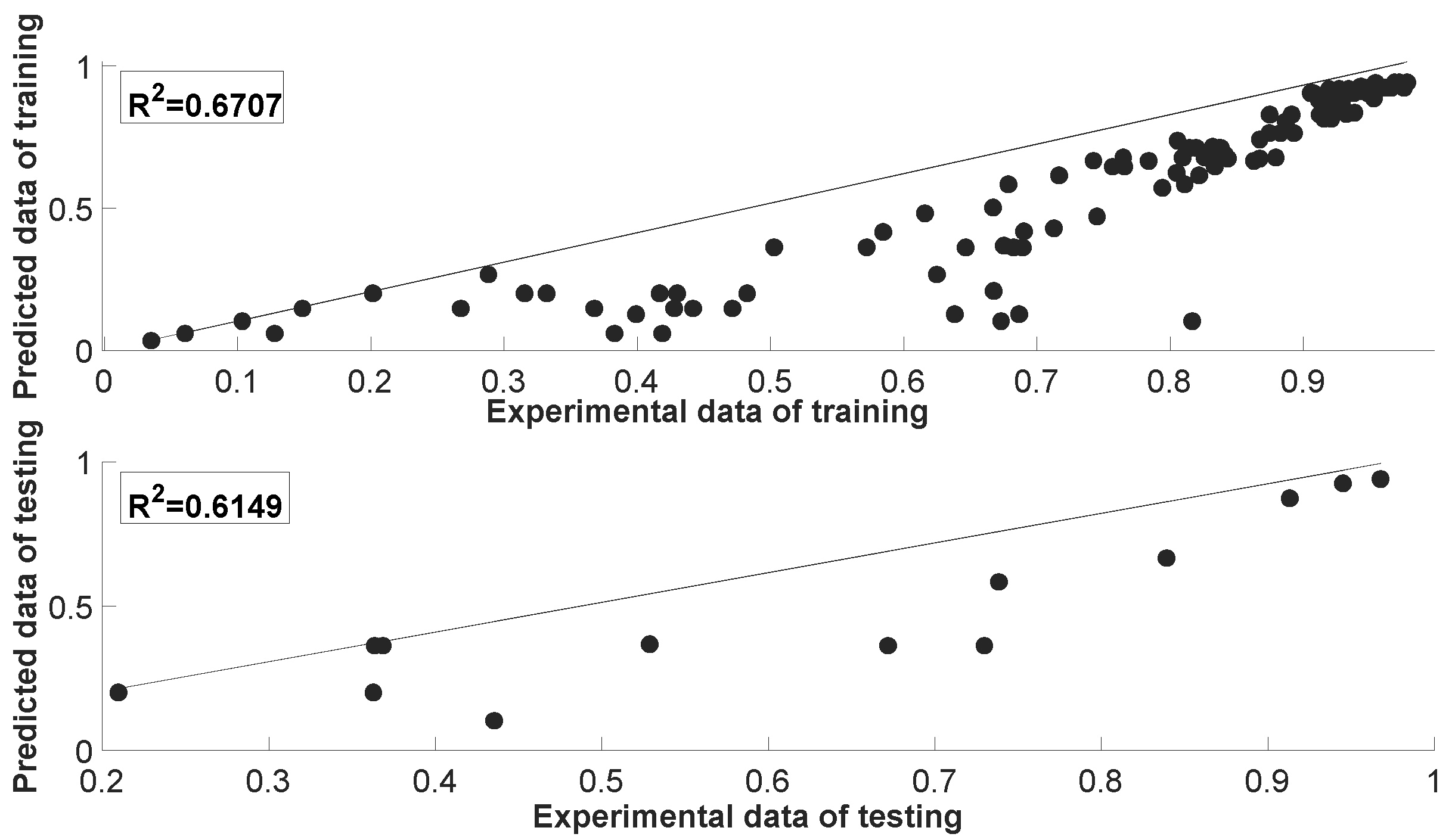
The input and output data used in the KNN algorithm are given in Section 2.5. The performance metrics of MSE, PSNR, RMSE, NRMSE and MAPE were used to evaluate the performance of the KNN algorithm. The data used in the KNN algorithm were determined as 90% training data and 10% test data. With the KNN algorithm, the best prediction results were made according to distances and neighborhoods. The neighborhoods and distances of the KNN algorithm are given in Figure 9. The best neighbor and distance obtained in this study are given in Table 2. While the KNN algorithm estimated the losses caused by dust in PV panels, the neighborhood and distance were obtained as 10 and seuclide, respectively. The performance metrics of the KNN algorithm are given in Table 3. Figure 10 presents the predicted results and experimental results for the training and testing phases of KNN. The KNN algorithm predicted the losses due to dust of PV panels as 67.07% and 61.49% for the training and testing phases.
As seen in Figure 10, when the values between the dependent variable and the independent variable are taken into account, the deviation of the KNN algorithm is higher than the LSTM algorithm. As a result, it was observed that the performance of the KNN algorithm was lower than other algorithms in predicting power losses due to dust in PV panels.
When we compare the KNN algorithm and the LSTM algorithm in this study, the LSTM model has higher PSNR and , while it has lower MSE, RMSE, NRMSE and MAPE. The KNN model predicted the loss due to dust in PV panels with low accuracy.
3.3. Long Short-Term Memory of Results
The LSTM model estimated losses due to dust in PV panels. The input and output variables given in Section 2.5 were used in the LSTM model. Data from 365 samples were used in this study. In the LSTM model, 90% of the data were selected as training data and 10% as test data. The performance metrics of the LSTM model are the MSE, PSNR, RMSE, NRMSE and MAPE.
The performance metrics of the LSTM algorithm for testing and training are given in Table 4. The RMSE and loss of the LSTM model are given in Figure 11. The test and training results of the LSTM model for losses caused by dust in PV panels are presented in Figure 12. As seen in Table 4, the PSNR is higher in the training phase than in the testing phase. In the LSTM algorithm, the PSNR for training and testing is greater than other performance metrics. A large PSNR is evidence of good prediction performance. As seen in Figure 11, the losses and RMSE metric of the LSTM model for training and testing are minimum. While the RMSE value of the LSTM model was 0.0325 in training, the RMSE value was 0.0388 in the testing phase. As can be seen from the results, the RMSE value is close to 0 and the predicted value is close to the real value. As seen in Figure 12, the metric of the LSTM model in training and testing for losses caused by dust of PV panels were 0.9639 and 0.9551, respectively. The LSTM algorithm has shown a good performance in estimating the losses of PV panels due to dust.
As seen in the regression curve in Figure 12, the deviations between the dependent variable and the independent variable in the testing and training phases of the LSTM model are at a level close to the minimum. This shows that the estimated value is close to the real value.
3.4. Hybrid LSTM-KNN of Results
The hybrid deep LSTM-KNN model was used to predict losses due to dust in PV panels. The hybrid deep learning model was designed using long short-term memory and the Knearest neighbour algorithm. The hybrid deep learning architecture is given in Figure 7. In this section, the data set used in the LSTM and KNN model is used. Similar to other models, the input variables of the hybrid deep learning model are meteorological data, while the output variable is the losses caused by dust in PV panels. The parameters of the hybrid LSTM-KNN model are given in Table 5. The MSE, PSNR, RMSE, NRMSE and MAPE were used to evaluate the performance of the hybrid deep learning model. The performance metrics of the hybrid deep learning model are given in Table 6. As seen in Table 6, the PSNR in the testing and training of the hybrid LSTM-KNN model is higher than that of the LSTM and KNN models. In addition, the MSE, RMSE, NRMSE and MAPE of the hybrid deep LSTM-KNN model in testing and training are smaller than the LSTM and KNN models.
Figure 13 presents the predicted results and experimental results for the training and testing phases of the hybrid LSTM-KNN model. As seen in Figure 13, deviations between the dependent variable and the independent variable are minimal. The hybrid LSTM-KNN algorithm proved to have good prediction success in power losses due to dust in PV panels.The RMSE and loss of the hybrid deep LSTM-KNN model are given in Figure 14. As seen in Figure 14, the RMSE is minimum and the prediction data are very close to the real data. The hybrid LSTM-KNN model achieved RMSE values of 0.0134 and 0.0237 for testing and training, respectively. Losses and RMSE values were close to zero. These results showed that the hybrid LSTM-KNN model had good prediction success. The performance metrics of all models are given in Figure 15. In Figure 15a, the hybrid LSTM-KNN model in the training phase has a larger PSNR and R-value than other models. In addition, the MSE, RMSE, NRMSE and MAPE values of the hybrid LSTM-KNN model are smaller than other prediction models. In Figure 15b, the performance of the model in the hybrid LSTM-KNN test phase was similar to the training phase. As a result, the deep hybrid LSTM-KNN model has a better prediction performance than LSTM and KNN models.
A Taylor diagram is a method that statistically measures the degree of similarity between pairs of interests. The first area of interest is the reference area, while the second is the test area. It measures the similarity between the reference area and the test area. However, it shows the root mean square (RMS) difference, correlation coefficient and standard deviation between these two areas [38].
Figure 16 shows the Taylor diagram for the LSTM, KNN and hybrid LSTM-KNN models. As can be seen in Figure 16, in both the test and training phases, the hybrid LSTM-KNN model was closest to the actual value, while the KNN model was far from the real value.
In the literature, the following studies were available to estimate the power loss due to dust of PV panels. The algorithms used were ELM, ANN, ANFIS, hybrid CNN-LSTM, BNN, Random forest and MLR. The performance metrics for these algorithms were , MSE, RMSE, R, NRMSE and MAPE. Adıgüzel et al. [11] and Pavan et al. [16] estimated that the dust-related losses of PV panels were 99.803% and 99.92%, respectively. In the current study, the power loss due to dust was estimated at 98.22%. As seen in the literature, there were not many hybrid algorithms that predicted the power losses of PV panels due to dust. Jamil et al. [15] used a hybrid CNN-LSTM algorithm to estimate the power losses of PV panels due to dust and obtained a RMSE and MAPE of 0.00385 and 0.28474. In the current study, the RMSE and MAPE were 0.0237 and 4.3873, respectively. Jamil et al. [15]’s hybrid study was better than the current study. However, the performance of the current study was better than all other studies in the literature (Table 7).
4. Conclusions
In this study, we aimed to compare the performance of the LSTM, KNN and hybrid deep learning models used to predict losses caused by dust in PV panels. The hybrid deep learning model was created from the LSTM and KNN algorithms. Sensitivity analysis was performed to evaluate losses caused by dust in PV panels. The MSE, RMSE, NRMSE, MAPE, PSNR and were used to evaluate the performance of the models. The input variables of the model were selected as time, sunshine duration, humidity, ambient temperature and solar radiation. The output variable of the model is the losses of PV panels due to dust. Hybrid LSTM-KNN, LSTM and KNN models predicted the loss due to dust in PV panels at 98.22%, 95.51% and 61.49%, respectively. Among the variables affecting the loss due to dust in PV panels, the most important variable is solar radiation. It affected the loss due to dust in PV panels by 96.32%.
As a result of this study, it has been proven that power losses of PV panels due to dust can be predicted with the hybrid LSTM-KNN algorithm. The better performance of the hybrid LSTM-KNN algorithm over the LSTM and KNN algorithms increased the prediction value. Estimating the power losses of PV panels due to dust can contribute to the calculation of energy costs produced by PV power plants. In addition, the finding that solar radiation is one of the most important pieces of meteorological data affecting the power losses of PV panels due to dust can aid the manufacturer in terms of location estimation during the installation phase of PV panels. The hybrid LSTM-KNN algorithm can be used to estimate the amount of dust accumulated in PV panels and to predict the short- and long-term power of these panels. However, we could not shorten the running time of the hybrid LSTM-KNN algorithm and we saw that this time was relatively longer compared to other hybrid algorithms.
Funding
This research received no external funding.
Institutional Review Board Statement
Not applicable.
Informed Consent Statement
Not applicable.
Data Availability Statement
Data are contained within the article.
Conflicts of Interest
The author declares that they have no known competing financial interests or personal relationships that could have appeared to influence the work reported in this paper.
References
- Sampaio, P.G.V.; González, M.O.A. Photovoltaic solar energy: Conceptual framework. Renew. Sustain. Energy Rev. 2017, 74, 590–601. [Google Scholar] [CrossRef]
- Ganti, P.K.; Naik, H.; Barada, M.K. Environmental impact analysis and enhancement of factors affecting the photovoltaic (PV) energy utilization in mining industry by sparrow search optimization based gradient boosting decision tree approach. Energy 2022, 244, 122561. [Google Scholar] [CrossRef]
- Siecker, J.; Kusakana, K.; Numbi, E.B. A review of solar photovoltaic systems cooling technologies. Renew. Sustain. Energy Rev. 2017, 79, 192–203. [Google Scholar] [CrossRef]
- Fan, S.; Wang, Y.; Cao, S.; Zhao, B.; Sun, T.; Liu, P. A deep residual neural network identification method for uneven dust accumulation on photovoltaic (PV) panels. Energy 2022, 239, 122302. [Google Scholar] [CrossRef]
- Sayyah, A.; Horenstein, M.N.; Mazumder, M.K. Energy yield loss caused by dust deposition on photovoltaic panels. Solar Energy 2014, 107, 576–604. [Google Scholar] [CrossRef]
- Fan, S.; Wang, Y.; Cao, S.; Sun, T.; Liu, P. A novel method for analyzing the effect of dust accumulation on energy efficiency loss in photovoltaic (PV) system. Energy 2021, 234, 121112. [Google Scholar] [CrossRef]
- Hussain, A.; Batra, A.; Pachauri, R. An experimental study on effect of dust on power loss in solar photovoltaic module. Renew. Wind. Water Sol. 2017, 4, 9. [Google Scholar] [CrossRef]
- Chen, J.; Pan, G.; Ouyang, J.; Ma, J.; Fu, L.; Zhang, L. Study on impacts of dust accumulation and rainfall on PV power reduction in East China. Energy 2020, 194, 116915. [Google Scholar] [CrossRef]
- Al-Kouz, W.; Al-Dahidi, S.; Hammad, B.; Al-Abed, M. Modeling and analysis framework for investigating the impact of dust and temperature on PV systems’ performance and optimum cleaning frequency. Appl. Sci. 2019, 9, 1397. [Google Scholar] [CrossRef]
- Hammad, B.; Al-Abed, M.; Al-Ghandoor, A.; Al-Sardeah, A.; Al-Bashir, A. Modeling and analysis of dust and temperature effects on photovoltaic systems’ performance and optimal cleaning frequency: Jordan case study. Renew. Sustain. Energy Rev. 2018, 82, 2218–2234. [Google Scholar] [CrossRef]
- Adıgüzel, E.; Özer, E.; Akgündoğdu, A.; Yılmaz, A.E. Prediction of dust particle size effect on efficiency of photovoltaic modules with ANFIS: An experimental study in Aegean region, Turkey. Solar Energy 2019, 177, 690–702. [Google Scholar] [CrossRef]
- Javed, W.; Guo, B.; Figgis, B. Modeling of photovoltaic soiling loss as a function of environmental variables. Solar Energy 2017, 157, 397–407. [Google Scholar] [CrossRef]
- Simal Pérez, N.; Alonso-Montesinos, J.; Batlles, F.J. Estimation of soiling losses from an experimental photovoltaic plant using artificial intelligence techniques. Appl. Sci. 2021, 11, 1516. [Google Scholar] [CrossRef]
- Zitouni, H.; Azouzoute, A.; Hajjaj, C.; El Ydrissi, M.; Regragui, M.; Polo, J.; Oufadel, A.; Bouaichi, A.; Ghennioui, A. Experimental investigation and modeling of photovoltaic soiling loss as a function of environmental variables: A case study of semi-arid climate. Solar Energy Mater. Sol. Cells 2021, 221, 110874. [Google Scholar] [CrossRef]
- Jamil, I.; Lucheng, H.; Iqbal, S.; Aurangzaib, M.; Jamil, R.; Kotb, H.; Alkuhayli, A.; AboRas, K.M. Predictive evaluation of solar energy variables for a large-scale solar power plant based on triple deep learning forecast models. Alex. Eng. J. 2023, 76, 51–73. [Google Scholar] [CrossRef]
- Pavan, A.M.; Mellit, A.; De Pieri, D.; Kalogirou, S.A. A comparison between BNN and regression polynomial methods for the evaluation of the effect of soiling in large scale photovoltaic plants. Appl. Energy 2013, 108, 392–401. [Google Scholar] [CrossRef]
- Velásquez, R.M.A.; Ezcurra, T.T.P. Dust analysis in photo-voltaic solar plants with satellite data. Ain Shams Eng. J. 2023, 15, 102314. [Google Scholar] [CrossRef]
- Available online: https://www.saruhanli.bel.tr/saruhanli-icerik.php?icerik_id=52 (accessed on 15 September 2023).
- Available online: https://tr.weatherspark.com/y/94309/Saruhanl%C4%B1-T%C3%BCrkiye-Ortalama-Hava-Durumu-Y%C4%B1l-Boyunca (accessed on 25 September 2023).
- Available online: https://saruhanli.bel.tr/senar/production/upload/752276338.pdf (accessed on 25 September 2023).
- Available online: https://www.mgm.gov.tr/kurumsal/istasyonlarimiz.aspx (accessed on 1 October 2023).
- Available online: https://csb.gov.tr/sss/hava-yonetimi (accessed on 14 October 2023).
- Moeinossadat, S.R.; Ahangari, K.; Shahriar, K. Calculation of maximum surface settlement induced by EPB shield tunnelling and introducing most effective parameter. J. Cent. South Univ. 2016, 23, 3273–3283. [Google Scholar] [CrossRef]
- Moeinossadat, S.R.; Ahangari, K.; Shahriar, K. Control of ground settlements caused by EPBS tunneling using an intelligent predictive model. Indian Geotech. J. 2018, 48, 420–429. [Google Scholar] [CrossRef]
- Adithiyaa, T.; Chandramohan, D.; Sathish, T. Optimal prediction of process parameters by GWO-KNN in stirring-squeeze casting of AA2219 reinforced metal matrix composites. Mater. Today Proc. 2020, 21, 1000–1007. [Google Scholar] [CrossRef]
- Zhang, Z.; Jiang, T.; Li, S.; Yang, Y. Automated feature learning for nonlinear process monitoring–An approach using stacked denoising autoencoder and k-nearest neighbor rule. J. Process Control 2018, 64, 49–61. [Google Scholar] [CrossRef]
- Liu, K.; Li, Z.; Yao, C.; Chen, J.; Zhang, K.; Saifullah, M. Coupling the k-nearest neighbor procedure with the Kalman filter for real-time updating of the hydraulic model in flood forecasting. Int. J. Sediment Res. 2016, 31, 149–158. [Google Scholar] [CrossRef]
- Yamaç, S.S.; Todorovic, M. Estimation of daily potato crop evapotranspiration using three different machine learning algorithms and four scenarios of available meteorological data. Agric. Water Manag. 2020, 228, 105875. [Google Scholar] [CrossRef]
- Song, X.; Liu, Y.; Xue, L.; Wang, J.; Zhang, J.; Wang, J.; Jiang, L.; Cheng, Z. Time-series well performance prediction based on Long Short-Term Memory (LSTM) neural network model. J. Pet. Sci. Eng. 2020, 186, 106682. [Google Scholar] [CrossRef]
- Fan, D.; Sun, H.; Yao, J.; Zhang, K.; Yan, X.; Sun, Z. Well production forecasting based on ARIMA-LSTM model considering manual operations. Energy 2021, 220, 119708. [Google Scholar] [CrossRef]
- Nguyen, H.D.; Tran, K.P.; Thomassey, S.; Hamad, M. Forecasting and Anomaly Detection approaches using LSTM and LSTM Autoencoder techniques with the applications in supply chain management. Int. J. Inf. Manag. 2021, 57, 102282. [Google Scholar] [CrossRef]
- Liang, X.; Xie, Y.; Day, R.; Meng, X.; Wu, H. A data driven deep neural network model for predicting boiling heat transfer in helical coils under high gravity. Int. J. Heat Mass Transf. 2021, 166, 120743. [Google Scholar] [CrossRef]
- Karaman, Ö.A.; Ağır, T.T.; Arsel, İ. Estimation of solar radiation using modern methods. Alex. Eng. J. 2021, 60, 2447–2455. [Google Scholar] [CrossRef]
- Karaman, Ö.A. Prediction of Wind Power with Machine Learning Models. Appl. Sci. 2023, 13, 11455. [Google Scholar] [CrossRef]
- Chicco, D.; Warrens, M.J.; Jurman, G. The coefficient of determination R-squared is more informative than SMAPE, MAE, MAPE, MSE and RMSE in regression analysis evaluation. PeerJ Comput. Sci. 2021, 7, e623. [Google Scholar] [CrossRef]
- Niu, X.; Ma, J.; Wang, Y.; Zhang, J.; Chen, H.; Tang, H. A novel decomposition-ensemble learning model based on ensemble empirical mode decomposition and recurrent neural network for landslide displacement prediction. Appl. Sci. 2021, 11, 4684. [Google Scholar] [CrossRef]
- Tanyildizi, H. Prediction of compressive strength of nano-silica modified engineering cementitious composites exposed to high temperatures using hybrid deep learning models. Expert Syst. Appl. 2023, 241, 122474. [Google Scholar] [CrossRef]
- Simão, M.L.; Videiro, P.M.; Silva PB, A.; de Freitas Assad, L.P.; Sagrilo, L.V.S. Application of Taylor diagram in the evaluation of joint environmental distributions’ performances. Mar. Syst. Ocean. Technol. 2020, 15, 151–159. [Google Scholar] [CrossRef]
- Sharma, S.; Joshua Thomas, J.; Vasant, P. Performance Analysis and Effects of Dust & Temperature on Solar PV Module System by Using Multivariate Linear Regression Model. In Artificial Intelligence for Renewable Energy and Climate Change; Wiley: Hoboken, NJ, USA, 2022; pp. 217–275. [Google Scholar] [CrossRef]
Figure 1.
Google earth view of Saruhanlı district [20].
Figure 1.
Google earth view of Saruhanlı district [20].

Figure 2.
Location plan.

Figure 3.
Powers of inverters in SEM4.

Figure 4.
K-nearest neighbor network architecture.

Figure 5.
LSTM network architecture.

Figure 6.
Flow diagram of the algorithm.

Figure 7.
Network structure of hybrid deep learning model.

Figure 8.
The sensitivity analysis of the results.

Figure 9.
KNN neighborhoods and distances.

Figure 10.
The predicted results for the training and testing stages of KNN and the experimental results.
Figure 10.
The predicted results for the training and testing stages of KNN and the experimental results.

Figure 11.
RMSE and losses for testing and training of the LSTM model.

Figure 12.
The predicted results for the training and testing stages of LSTM and the experimental results.
Figure 12.
The predicted results for the training and testing stages of LSTM and the experimental results.

Figure 13.
The predicted results for the training and testing stages of hybrid LSTM-KNN and the experimental results.
Figure 13.
The predicted results for the training and testing stages of hybrid LSTM-KNN and the experimental results.

Figure 14.
RMSE and loss of the hybrid LSTM-KNN model.

Figure 15.
Radar chart of performance metrics of LSTM, KNN and hybrid LSTM-KNN models. (a) Training; (b) Testing.
Figure 15.
Radar chart of performance metrics of LSTM, KNN and hybrid LSTM-KNN models. (a) Training; (b) Testing.

Figure 16.
Taylor diagram.


| Days | Sunshine Duration (Hours) | Humidity | Temperature (°C) | Solar Radiation | P(kW) |
|---|---|---|---|---|---|
| 1 | 0.3 | 91.3 | 11.2 | 0.9 | 51.28 |
| 2 | 0.6 | 89.3 | 9.7 | 1.3 | 72.22 |
| 3 | 1.7 | 90.6 | 7.2 | 1 | 43.16 |
| 4 | 0 | 89.1 | 7.5 | 1.3 | 102.4 |
| 5 | 1.3 | 80.7 | 12.5 | 1.1 | 123.95 |
| 6 | 3.2 | 88 | 8.3 | 1.4 | 118.6 |
| 7 | 2.1 | 89.5 | 8.4 | 1.3 | 79.65 |
| 8 | 0.6 | 83 | 11.7 | 1.3 | 115,55 |
| 9 | 3 | 77 | 15.7 | 0.6 | 11.13 |
| 10 | 0.6 | 83.8 | 15.7 | 1.3 | 41.17 |
| 11 | 3 | 71.3 | 18 | 1.2 | 19.36 |
| 12 | 1.5 | 52.8 | 20.2 | 1.1 | 69.23 |
| 13 | 0 | 78.8 | 12.8 | 1.2 | 144.93 |
| 14 | 3.2 | 82.9 | 7.6 | 1.2 | 101.27 |
| 15 | 1.9 | 83.1 | 5.1 | 1.3 | 124.53 |
| 16 | 3.1 | 87.5 | 1.4 | 0.9 | 45.43 |
| 17 | 0.3 | 84.2 | 2 | 1.3 | 124.59 |
| 18 | 0.6 | 72.7 | 1.6 | 1.4 | 153.84 |
| 19 | 4.2 | 74.2 | −0.3 | 1.5 | 163.03 |
| 20 | 4.5 | 77.6 | −0.6 | 1.3 | 176.26 |
| 21 | 4.6 | 82.3 | 1 | 1.5 | 109,5 |
| 22 | 1.7 | 88.2 | 3 | 1 | 63.15 |
| 23 | 0 | 87.7 | 7.3 | 1.2 | 40.82 |
| 24 | 0 | 79.9 | 12.9 | 1.3 | 82.9 |
| 25 | 0 | 73.8 | 14.5 | 0.9 | 44.07 |
| 26 | 0 | 69.8 | 15.5 | 1.8 | 37.77 |
| 27 | 1 | 77.4 | 11.5 | 0.9 | 27.04 |
| 28 | 0.4 | 87 | 3.4 | 1.3 | 56.56 |
| 29 | 0.2 | 86.1 | 2.6 | 1.4 | 145.34 |
| 30 | 2.8 | 87.9 | 8.1 | 0.8 | 9.07 |
| 31 | 0.3 | 86.2 | 9.4 | 1.6 | 128.87 |
Table 2.
The distances and neighboring relations of the KNN algorithm.
| NumNeighbors(K) | Distance |
|---|---|
| 10 | Seuclidean |
Table 3.
Performance metrics of the KNN algorithm.
| Performance Metrics | Training | Testing |
|---|---|---|
| MSE | 0.0344 | 0.0344 |
| PSNR | 14.6327 | 14.6394 |
| RMSE | 0.1855 | 0.1854 |
| NRMSE | 0.1968 | 0.2446 |
| MAPE | 20.6954 | 23.2731 |
| 0.6707 | 0.6149 |
Table 4.
Performance metrics of the LSTM algorithm.
| Performance Metrics | Training | Testing |
|---|---|---|
| MSE | 0.0011 | 0.0015 |
| PSNR | 29.7727 | 28.2251 |
| RMSE | 0.0325 | 0.0388 |
| NRMSE | 0.0344 | 0.0512 |
| MAPE | 6.4598 | 6.9112 |
| 0.9639 | 0.9551 |
Table 5.
Hybrid LSTM-KNN parameters.
| Elapsed Time | Epoch | Iteration | Frequency | Hardware Resource | Learning Rate Schedule | Learning Rate |
|---|---|---|---|---|---|---|
| 28 Sec | 2000 | 2000 | 50 Iterations | Single GPU | Piecewise | 2 × 10⁻⁶ |
Table 6.
Performance metrics of the hybrid LSTM-KNN algorithm.
| Performance Metrics | Training | Testing |
|---|---|---|
| MSE | 1.7915 × 10⁻⁴ | 5.6199 × 10⁻⁴ |
| PSNR | 37.4679 | 32.5027 |
| RMSE | 0.0134 | 0.0237 |
| NRMSE | 0.0142 | 0.0313 |
| MAPE | 2.7509 | 4.3873 |
| 0.9963 | 0.9822 |
Table 7.
Literature comparison.
| Reference | Model | MSE | RMSE | R | NRMSE | MAPE | |
|---|---|---|---|---|---|---|---|
| Kouz et al. [9] | ELM | 91.42% | 0.0462 | - | - | - | |
| Hammad et al. [10] | ANN | 90.0% | 5.7 | - | - | - | |
| Adıgüzel et al. [11] | ANFIS | 99.803% | - | 0.87098 | - | - | |
| Javed et al. [12] | ANN | 53.7% | 0.0038 | - | - | - | |
| Perez et al. [13] | ANN | - | - | - | 91% | 6.79 | |
| Zitouni et al. [14] | ANN | 81.3% | - | 0.026 | - | - | |
| Jamil et al. [15] | Hybrid CNN-LSTM | - | - | 0.00385 | - | - | 0.28478 |
| Pavan et al. [16] | BNN | 99.92% | - | 0.22 | 99.96% | - | 2.3 |
| Valasquezand Ezcurra [17] | Random forest | 0.88% | 0.07 | - | - | - | - |
| Sharma et al. [39] | MLR | 91% | - | - | - | - | - |
| Presend study | Hybrid LSTM-KNN | 98.22% | 5.6199 × 10⁻⁴ | 0.0237 | 99.10% | 0.0313 | 4.3873 |
Disclaimer/Publisher’s Note: The statements, opinions and data contained in all publications are solely those of the individual author(s) and contributor(s) and not of MDPI and/or the editor(s). MDPI and/or the editor(s) disclaim responsibility for any injury to people or property resulting from any ideas, methods, instructions or products referred to in the content. |
© 2024 by the author. Licensee MDPI, Basel, Switzerland. This article is an open access article distributed under the terms and conditions of the Creative Commons Attribution (CC BY) license (https://creativecommons.org/licenses/by/4.0/).
Share and Cite
MDPI and ACS Style
Tanyıldızı Ağır, T. Prediction of Losses Due to Dust in PV Using Hybrid LSTM-KNN Algorithm: The Case of Saruhanlı. Sustainability 2024, 16, 3581. https://doi.org/10.3390/su16093581
AMA Style
Tanyıldızı Ağır T. Prediction of Losses Due to Dust in PV Using Hybrid LSTM-KNN Algorithm: The Case of Saruhanlı. Sustainability. 2024; 16(9):3581. https://doi.org/10.3390/su16093581
Chicago/Turabian StyleTanyıldızı Ağır, Tuba. 2024. "Prediction of Losses Due to Dust in PV Using Hybrid LSTM-KNN Algorithm: The Case of Saruhanlı" Sustainability 16, no. 9: 3581. https://doi.org/10.3390/su16093581
Note that from the first issue of 2016, this journal uses article numbers instead of page numbers. See further details here.