Understanding the Role of Built Environment in Reducing Vehicle Miles Traveled Accounting for Spatial Heterogeneity

Abstract

In recent years, increasing concerns over climate change and transportation energy consumption have sparked research into the influences of urban form and land use patterns on motorized travel, notably vehicle miles traveled (VMT). However, empirical studies provide mixed evidence of the influence of the built environment on travel. In particular, the role of density after controlling for the confounding factors (e.g., land use mix, average block size, and distance from CBD) still remains unclear. The object of this study is twofold. First, this research provides additional insights into the effects of built environment factors on the work-related VMT, considering urban form measurements at both the home location and workplace simultaneously. Second, a cross-classified multilevel model using Bayesian approach is applied to account for the spatial heterogeneity across spatial units. Using Washington DC as our study area, the home-based work tour in the AM peak hours is used as the analysis unit. Estimation results confirmed the important role that the built environment at both home and workplace plays in affecting work-related VMT. In particular, the results reveal that densities at the workplace have more important roles than that at home location. These findings confirm that urban planning and city design should be part of the solution in stabilizing global climate and energy consumption.

1. Introduction

With the growth in automobile use and increase in daily vehicle miles traveled (VMT), transportation energy consumption and air pollution are significantly increasing. The average annual VMT per household increased by 50 percent between the year 1970 and 2005 in United States [1]. Urban transportation is responsible for about 30 percent of the total greenhouse gases nation-wide [2]. There are two potential solutions that have been proposed to deal with the burning issues of the growth of energy consumption and emissions. One potential solution can achieve the greenhouse gas reduction targets through sustainable mobility (e.g., introduction of low-carbon fuels and new technologies that increase fuel efficiency). Another way to alleviate greenhouse gas emission is through sustainable urbanism (redesigning our cities so there is less need to drive). Promoting the compact, high-density, mixed-use, pedestrian-friendly, and transit-oriented development are widely considered as effective planning strategies to reduce the dependence on automobiles. Adapting from Mui et al. [3] and Cervero et al. [4], greenhouse emission reductions could come from the combination of the two potential solutions as shown in Equation (1).

(1)

In Growing Cooler, Ewing et al. [5] found that the transportation sector cannot achieve 2050 emission targets in U.S. merely through improvements in vehicle and fuel technology. It is necessary to find a way to sharply reduce the growth in vehicle miles driven across the nation’s sprawling urban areas. Many previous studies have focused on the impact of selected built environment (e.g., land use density, land use mix, street network density, block sizes, et al.) on selected travel dimensions (e.g., car ownership, number of trips, mode choice, et al.). In recent years, a substantial body of literature examines the connection between the built environment and VMT to address the importance of land use policies in VMT and travel related energy consumption reduction [4,6,7]. Cervero and Murakami [4] revealed that higher population densities are strongly associated with reduced VMT, on the basis of data from 370 U.S. urbanized areas using structural equation modeling. Ewing and Cervero [6] found VMT to be more strongly influenced by regional accessibility than density based on a meta-analysis. Chen et al. [8] analyzed the impact of the built environment on commuter mode choice decision using home-based work tour as the analysis unit. Employment density at work ends is found to be more important than densities at home ends.

The aforementioned studies have found significant relationships between density and automobile use. However, a small number of studies found the impact of density on travel to be negligible [7]. The role of density on reducing automobile use still remains unclear [8]: can density by itself be a useful policy tool or do other factors that go along with the density matter? Different methodologies, data, and geographic scales lead to mixed evidence of the influence of the built environment on travel behavior. In contrast to the policy measures such as congestion pricing and gasoline tax, land use planning is widely considered as a fundamental and long-term strategy to reduce the dependence on automobiles because it determines the basic spatial settings for various activities [5,9].

Studies on the relationship between land use and travel behavior are often conducted at aggregate geographic units such as the census tract, traffic analysis zone (TAZ) or the zip code level, probably due to land use data availability. Information about individual interactions can be found in many existing datasets that also contain other unobserved contextual behavior [10]. For example, individuals travel in certain neighborhoods (e.g., living in the same area) might have similar travel behavior. In this spatial clustering context, it is important to recognize and address the between-place heterogeneity [11]. Ignoring the spatial heterogeneity in travel behavior studies generally results in inconsistent parameter estimation. To accommodate the spatial context, the multilevel/hierarchical modeling framework has been recently applied [9,12,13,14,15,16]. Hong et al. [9] and Zhang et al. [14] examined the effects of built environment factors at home location on VMT by employing Bayesian multilevel model. Antipova et al. [16] used a multilevel modeling approach to examine the effects of neighborhood land use types at TAZ level and socio-demographic attributes on commuting distance and time. These applications to travel behavior suggest that ignoring the spatial issue can lead to an inferior data fit and generate erroneous conclusions. A body of literature shows that land use factors at the workplace may also have significant effects on work related travel behavior [6]. However, the dimension of built environment at the workplace was neglected in the current multilevel modeling literature, probably due to its complex estimation simultaneously handling more than one dimension within a multilevel framework. In addition, most existing studies still used single trip as the analysis unit [14,16,17]. However, trips are conceived as isolated travel patterns, which can not reflect the real travel behavior. In fact, it is very likely for people to make a series of trips (chained trips) between their origins and final destinations, which makes travel more complicated. The housewife, for example, may pick up children from school on her way to go grocery shopping [18].

This aim of this study is to provide additional insights into the linkages between built environment and the work-related VMT, using a cross-classified multilevel model with built environment factors measured at both home location and workplace to account for the spatial heterogeneity across spatial units. Meanwhile, the role of three core dimensions of built environment (density, diversity, and design) on reducing the work-related VMT in Washington DC can be investigated. Due to lack of attitude data, the residential self-selection issue is addressed indirectly by controlling for the socioeconomic and demographics information of individuals [19,20]. The remainder of this paper is organized as follows. The next section presents the data source and built environment measures. The third section presents the modeling approach used for the analysis. The model results are explained in the fourth section. Finally, the conclusions are provided and the future directions of this paper are proposed.

2. Data Source and Built Environment Measures

The travel data used in this study is drawn from the Maryland and Washington DC Regional Household Travel Survey (HTS), which was conducted by the Baltimore Metropolitan Council (BMC) and Transportation Planning Board (TPB) at the Metropolitan Washington Council of Governments (MWCOG) during 2007–2008. Data for the survey was collected from randomly selected households. Each household completed a travel diary that documented the activities of all household members on an assigned day. As with most household travel survey, detailed socio-demographic and trip information for each person were collected.

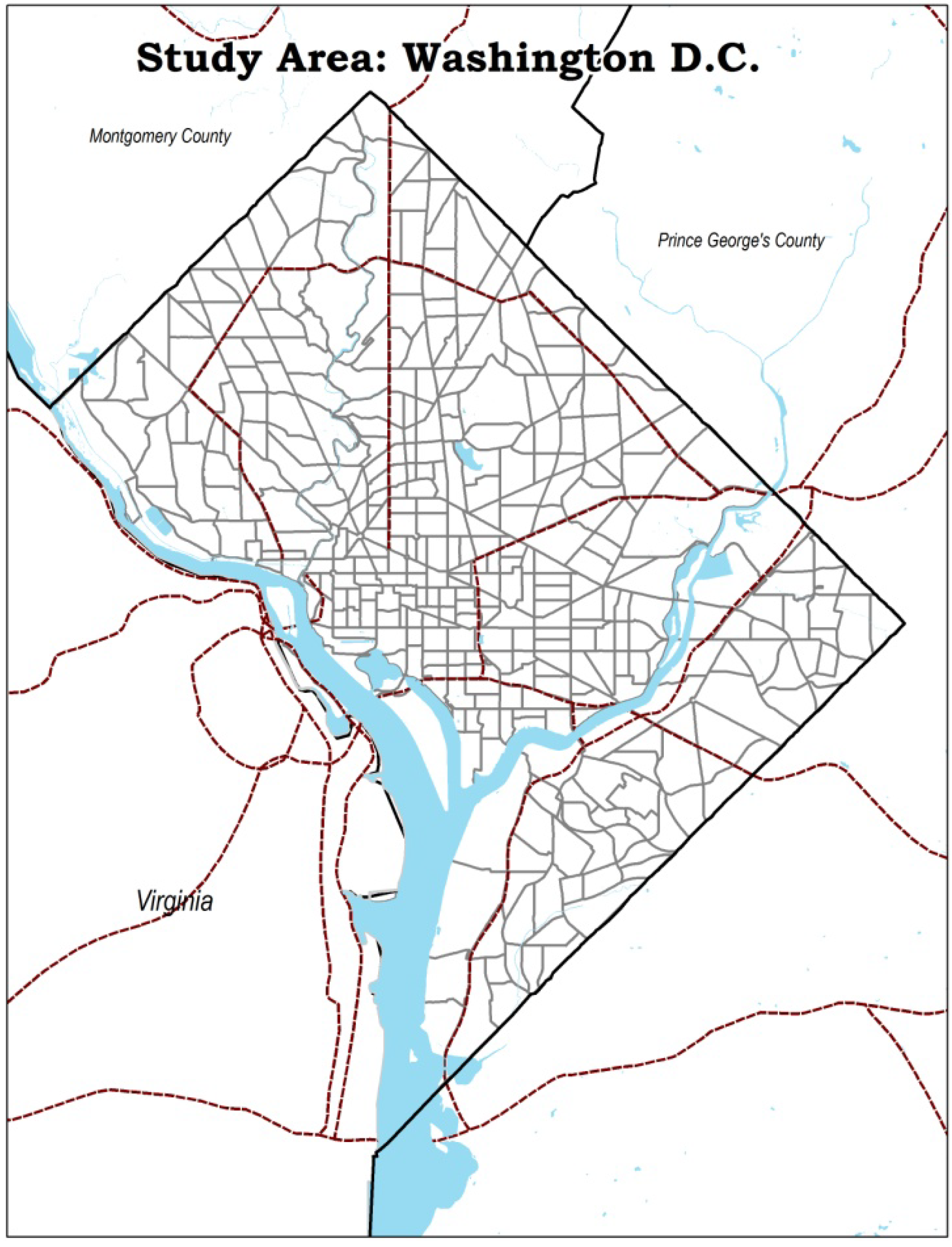
Washington DC is the study area as it is one of the densest metropolitan areas in the United States, as shown in Figure 1. Its built environment and transportation services are relatively friendly for non-motorized travel. In fact, the Washington DC region is a national leader in promoting transit-oriented development (TOD) whose transit system consists of a variety of modes, mainly subway, commuter rail, regular bus, and taxi. The system provides the residents with sufficient mobility and accessibility. In this way, it becomes important to model and find the effects of land use pattern on travel behavior. Urban form data were collected from two major sources: the MWCOG and the US Census. These datasets include population, employment information, different land use types and acreage in each TAZ. We calculated residential density, employment density, land use mix, average block size, and distance from CBD in ArcGIS 10.0 to represent the built environment measurements at the TAZ level. All the built environment factors used in this study are summarized in Table 1. Entropy measure that indicates the extent of mixed land development (e.g., houses, shops, restaurants, offices) is widely used in travel studies. In this paper, the entropy index was computed based on four different land use categories at the TAZ level, as shown in Equation (2).

(2)

where P_i is the proportion of land use type i in each TAZ, and n is the number of different land use types (residential, service, retail, and others). The value of land use mix index ranges from 0–1 and captures how evenly the residential, service, retail and other areas are distributed within the TAZ. Higher values of land use mix indicate a more balanced land use pattern.

Figure 1. Study area of Washington DC.

Figure 1. Study area of Washington DC.

Table 1. Built environment factors.

Measure	Definition at TAZ level
Residential density	Population/Area size (persons/acre)
Employment density	Employment/Area size (jobs/acre)
Land use mix (entropy)	Mixture of residential, service, retail, and other employment land use types
Average block size	Average block size within TAZ (sq. mi.)
Distance from CBD	Straight line distance from CBD (mile)

Table 1. Built environment factors.

Measure	Definition at TAZ level
Residential density	Population/Area size (persons/acre)
Employment density	Employment/Area size (jobs/acre)
Land use mix (entropy)	Mixture of residential, service, retail, and other employment land use types
Average block size	Average block size within TAZ (sq. mi.)
Distance from CBD	Straight line distance from CBD (mile)

In this study, we examine the travel behavior of two motorized travel modes including automobile (drive-alone or shared-ride) and transit (subway, commuter rail, or local bus) for the commuters who made a tour from home to workplace in the AM peak hours (5 a.m.–10 a.m.) on the survey day. A tour is defined as a sequence of trips that starts at home and ends at the workplace. In this study, the tour-based VMT is calculated as the total VMT for each person over the whole work tour by summing up the travel distances of all trips of the work tour. As for auto trips, the VMT of each trip is weighted by the number of people sharing the vehicle. For travelers who are taking transit, it is hard to obtain the number of passengers. In this study, we divided the trip distance by the national average passenger load in a conventional bus in 2006, which is 9.2 [9,14,21]. Tours made entirely by non-motorized modes (e.g., walking or bicycling) and respondents who are less than 16 years old are excluded. The final sample comprises 980 observations from 817 households and 980 commuters. These tours originate at 202 home zones and end at 346 work zones. Fifty-two percent of the tours have at least one stop between the staring home location and the ending workplace. The average commuting distance is 6.37 miles with the standard deviation of 5.969. The average household size is 2.02 with a maximum of 6 and almost 34% of the respondents in the region live alone. The average sample age is about 43 years old. Over 70% of the respondents have no students in their households. Nearly 50% of the household have two workers. Sixteen and a half percent of samples have no vehicles and 32.7% of the households own two or more vehicles. The mean household income is between $75,000 and $100,000. It can be seen that the sample consists of a high percentage of wealthy people. The mode choice shares in the sample are as follows: automobile (52.1%) and transit (47.9%). Table 2 shows descriptive statistics of the sample data used in this study.

Table 2. Descriptive statistics of the sample data for the tours from home to work (N = 980).

Variable Name	Variable Description	Mean	St. Dev.
Household size	Number of persons in household	2.02	1.013
Household students	Number of students in household	0.41	0.731
Household workers	Number of workers in household	1.56	0.568
Number of vehicles	Number of household vehicles available	1.25	0.860
Household income	Income1: household income is less than $40,000 (1 = yes)	0.10	0.302
	Income2: household income is between $40,000 and $150,000 (1 = yes)	0.65	0.477
	Income3: household income is equal to or more than $150,000 (1 = yes)	0.25	0.431
Age	Age of respondents in years	42.69	13.018
Gender	Male (1 = yes)	0.46	0.498

Note: 980 tours, 817 households, 980 persons, 202 residential zones, 346 workplace zones.

Table 2. Descriptive statistics of the sample data for the tours from home to work (N = 980).

Variable Name	Variable Description	Mean	St. Dev.
Household size	Number of persons in household	2.02	1.013
Household students	Number of students in household	0.41	0.731
Household workers	Number of workers in household	1.56	0.568
Number of vehicles	Number of household vehicles available	1.25	0.860
Household income	Income1: household income is less than $40,000 (1 = yes)	0.10	0.302
	Income2: household income is between $40,000 and $150,000 (1 = yes)	0.65	0.477
	Income3: household income is equal to or more than $150,000 (1 = yes)	0.25	0.431
Age	Age of respondents in years	42.69	13.018
Gender	Male (1 = yes)	0.46	0.498

Note: 980 tours, 817 households, 980 persons, 202 residential zones, 346 workplace zones.

3. Model Specification

The multilevel modeling approach is used to account for the hierarchical structure of the data in this study. Since individuals are nested within TAZs, people who reside in the same TAZ have more similar behavior than those living in other TAZs. By specifying individual commuters nested within TAZs, the multilevel model can separate the effects of built environment on commuter travel behavior from individual attributes [15,16]. The built environment measures from home location and the workplace are both included in our study. However, commuters are cross-classified by home location and workplace at the TAZ level. For example, level origin is the home location that the individual lives in and level destination is the workplace that an individual goes to. The structure of the origin and destination dataset is not nested. Therefore, to capture both the impacts of built environment at origin and destination on travel behavior, the cross-classified multilevel model by allowing for varying intercepts is used in this study. Varying intercepts are estimated by using both individual and group information. The dependent variable VMT_qhw that an individual q (q = 1, 2, …, Q) in residence zone h (h = 1, 2, …, H) and workplace zone w (w = 1, 2, …, W) associates with the work-related VMT can be written as below:

VMT_qhw = α_hw + β^TX_qhw + ε_qhw

(3)

And:

α_hw = φ + μ^TY_hw + γ^TZ_hw + ξ_h + δ_w

(4)

where X_qhwi, Y_hwi, Z_hwi represent the individual-associated attributes (household and individual factors), built environment measures at home location TAZs and workplace TAZs, respectively. α_hw is a varying intercept associated with the residence zone h and workplace zone w of an individual. β, φ, μ, and γ are fixed effect coefficients on the different levels. ε_qhw is an unobserved random term that represents idiosyncratic individual differences after allowing for differences due to observed individual characteristics and zone-level differences. ξ_h and δ_w are random terms that capture unobserved variations across home location zones and workplace zones, respectively. Here, ε_qhw, ξ_h, and δ_w are assumed to be normally and identically distributed:

(5)

Then, the final model with built environment factors measured at home location and workplace at TAZ level can be specified as below:

(6)

where varying intercept α_hwi is assumed to be normally and independently distributed with the expected value φ + μ^TY_hwi + γ^TZ_hwi and variance . Y_hw and Z_hw refer to group predictors measured at home-zone level and work-zone level.

A conventional varying intercept model can accommodate the spatial context in which individuals make travel decisions: spatial autocorrelation (correlation among individuals in the same home/work zones) and spatial heterogeneity (variations in impedance measures across zonal pairs). The correlation between two individuals in the same home location zone and workplace zone can be expressed by intra-class correlation coefficient (ICC) calculated by . For two individuals in the same home location zone, but in different workplace zones, the correlation between them can be calculated by . For two individuals in the same workplace zone, but in different home location zones, the correlation between them can be calculated by . The value of intra-class correlation ranges from 0–1. This index describes the spatial heterogeneity across TAZs in the relationship between travel behavior and its determinants. It also captures spatial autocorrelation among individuals residing within the same zone and recognizes the spatial heteroscedasticity [11]. In general, if the value of intra-class correlation combines the range of 0.10–0.25 or higher, there is a need to perform a multilevel analysis to account for the spatial heterogeneity.

The Bayesian estimation approach is employed for the cross-classified multilevel model because it has several advantages over other methods. First, it considers uncertainty in estimating parameters by simulating posterior distributions. Second, in contrast to the asymptotic maximum likelihood method, it is valid in small samples. In maximum likelihood estimation and hypothesis testing, the true value of the model parameters are viewed as fixed but unknown. It maximizes the likelihood of an unknown parameter θ when given the observed data y through the relationship L(θ|y) ∝ p(y|θ). Whereas Bayesian estimation approximates the posterior density of y, p(θ|y) ∝ p(θ)L(θ|y), where p(θ) is the prior distribution of θ, and p(θ|y) is the posterior density of θ given y. Conceptually, the posterior density of y given θ is the product of the prior distribution of θ and the likelihood of the observed data based on Bayes theorem below [22]:

(7)

In this study, non-information priori with a relatively flat distribution is employed because prior information does not exist. Using a new class of simulation techniques called Markov Chain Monte Carlo (MCMC), the joint posterior distributions can be computed [23]. Unlike a conventional interval, the Bayesian credible interval (C.I.) is interpreted as a probability statement about the parameter itself: a 95% Bayesian credible interval contains the true parameter value with approximately 95% certainty. If the 95% Bayesian credible interval of the posterior mean does not include zero, then it indicates that this effect is statistically significant at the 95% level.

4. Results

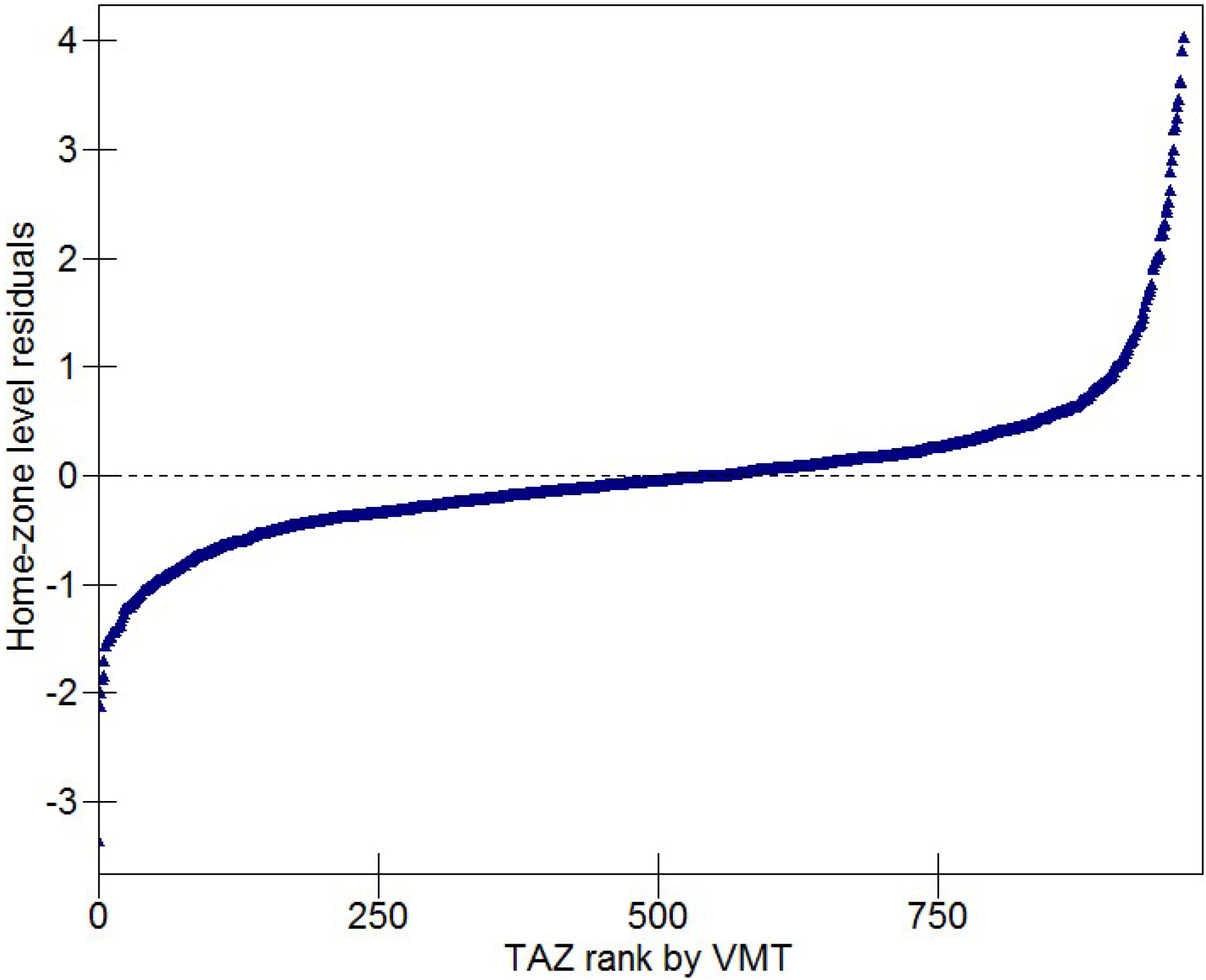
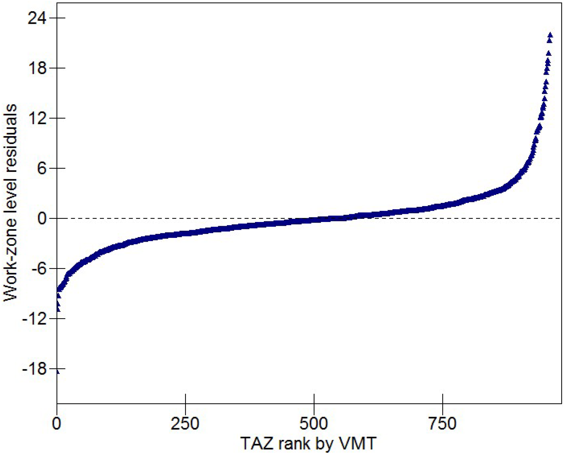
The residuals for ordered mean VMT by TAZs at the home-zone level and work-zone level are shown in Figure 2 and Figure 3, respectively. From the two figures, we can see the heterogeneous residuals of travelers living or working in different areas, indicating a possible spatial autocorrelation within the same group. Therefore, it is necessary to accommodate the spatial contexts to analyze the influences of built environment factors. The results of the cross-classified multilevel model are shown in Table 3. This presents empirical evidence of the impact of built environment on VMT per person. The 95% C.I. and 90% C.I. for each coefficient are displayed as the reference for significant level. As mentioned previously, if zero does not fall in the 95% C.I. for a parameter, the coefficient is statistically significant at the 95% level. With the Bayesian multilevel model method, the explained variance (R²) at the different levels is measured as a familiar summary of the fit of the model [9,14,24]. As shown in Table 3, the R² at the individual level, home-zone level, and work-zone level is 0.463, 0.504, and 0.874, respectively. This implies a good fit of the model. Meanwhile, some socio-demographic variables are found to be significant, and the signs of the coefficients are reasonable.

Figure 2. Home-zone level residuals for the vehicle miles traveled (VMT).

Figure 2. Home-zone level residuals for the vehicle miles traveled (VMT).

Figure 3. Work-zone level residuals for the VMT.

Figure 3. Work-zone level residuals for the VMT.

After controlling for the socio-demographic factors, only one built environment variable (i.e., Distance to CBD) at home location is significantly associated with work-related VMT at the 95% level. This result suggests that people tend to drive further if they live further away from the CBD area. This finding is intuitive since most of the employment concentrates in the CBD area that attracts people travel from different areas of the region. Average block size at home location attained a statistical significance at the 90% level. In general, a smaller block size indicates better street connectivity and that is friendly for non-motorized travel. However, somewhat surprisingly, increasing average block size at the residence zone is associated with more transit travel. This can be explained by the fact that most commuters living in suburbs trade off housing prices and transportation costs. Average block size acts as the proxy indicator of suburban neighborhoods. The subway and commuter rail system covers most of the case area and suburban commuters tend to take transit to work in the region.

Table 3. Model results of the cross-classified multilevel model using Bayesian approach (N = 980).

Variable	Bayesian Cross-Classified Multilevel Model
	Mean	Posterior S.D.	95% C.I.		90% C.I.
			Lower 2.5%	Upper 2.5%	Lower 5%	Upper 5%
Socio-demographic and control factors at individual level
Intercept	1.939	0.918	0.202	3.680	0.450	3.449
Household size	0.285	0.184	−0.054	0.658	0.003	0.612
Household students	−0.226	0.220	−0.655	0.192	−0.583	0.137
Household workers	−0.558	0.232	−1.028	−0.129	−0.950	−0.186
Number of vehicles	0.938	0.139	0.660	1.208	0.713	1.172
Income1	−0.178	0.360	−0.874	0.482	−0.786	0.392
Income3	0.931	0.251	0.430	1.417	0.518	1.344
Age	−0.003	0.008	−0.021	0.012	−0.017	0.009
Gender	0.200	0.200	−0.182	0.585	−0.128	0.527
Home location built environment at TAZ level
Residential density	−0.007	0.006	−0.019	0.006	−0.017	0.003
Employment density	0.003	0.003	−0.004	0.009	−0.003	0.008
Land use mix	−0.646	0.546	−1.761	0.392	−1.581	0.219
Average block size	−10.674	5.900	−21.952	0.638	−20.312	−1.200
Distance from CBD	0.442	0.162	0.143	0.752	0.182	0.709
Workplace built environment at TAZ level
Residential density	−0.055	0.017	−0.090	−0.021	−0.084	−0.027
Employment density	−0.006	0.003	−0.011	−0.001	−0.011	−0.002
Land use mix	−0.153	1.130	−2.534	1.893	−2.142	1.561
Average block size	19.996	4.353	11.408	28.645	12.932	27.254
Distance from CBD	0.481	0.047	0.389	0.576	0.404	0.558
Spatial heterogeneity parameters
	6.034	0.357	5.333	6.758	5.474	6.654
	0.360	0.172	0.091	0.767	0.120	0.687
	31.507	2.891	26.248	37.366	26.986	36.282
R2 individual level	0.463
R2 home-zone level	0.504
R2 work-zone level	0.874

Note: 980 tours, 817 households, 980 persons, 202 residential zones, 346 workplace zones.

Table 3. Model results of the cross-classified multilevel model using Bayesian approach (N = 980).

Variable	Bayesian Cross-Classified Multilevel Model
	Mean	Posterior S.D.	95% C.I.		90% C.I.
			Lower 2.5%	Upper 2.5%	Lower 5%	Upper 5%
Socio-demographic and control factors at individual level
Intercept	1.939	0.918	0.202	3.680	0.450	3.449
Household size	0.285	0.184	−0.054	0.658	0.003	0.612
Household students	−0.226	0.220	−0.655	0.192	−0.583	0.137
Household workers	−0.558	0.232	−1.028	−0.129	−0.950	−0.186
Number of vehicles	0.938	0.139	0.660	1.208	0.713	1.172
Income1	−0.178	0.360	−0.874	0.482	−0.786	0.392
Income3	0.931	0.251	0.430	1.417	0.518	1.344
Age	−0.003	0.008	−0.021	0.012	−0.017	0.009
Gender	0.200	0.200	−0.182	0.585	−0.128	0.527
Home location built environment at TAZ level
Residential density	−0.007	0.006	−0.019	0.006	−0.017	0.003
Employment density	0.003	0.003	−0.004	0.009	−0.003	0.008
Land use mix	−0.646	0.546	−1.761	0.392	−1.581	0.219
Average block size	−10.674	5.900	−21.952	0.638	−20.312	−1.200
Distance from CBD	0.442	0.162	0.143	0.752	0.182	0.709
Workplace built environment at TAZ level
Residential density	−0.055	0.017	−0.090	−0.021	−0.084	−0.027
Employment density	−0.006	0.003	−0.011	−0.001	−0.011	−0.002
Land use mix	−0.153	1.130	−2.534	1.893	−2.142	1.561
Average block size	19.996	4.353	11.408	28.645	12.932	27.254
Distance from CBD	0.481	0.047	0.389	0.576	0.404	0.558
Spatial heterogeneity parameters
	6.034	0.357	5.333	6.758	5.474	6.654
	0.360	0.172	0.091	0.767	0.120	0.687
	31.507	2.891	26.248	37.366	26.986	36.282
R2 individual level	0.463
R2 home-zone level	0.504
R2 work-zone level	0.874

Note: 980 tours, 817 households, 980 persons, 202 residential zones, 346 workplace zones.

In terms of the built environment at workplace, residential density, employment density, average block size, and distance from CBD are significantly associated with VMT at the 95% level. High residential and employment density at the workplace are associated with lower VMT. However, densities at home location did not show statistical relevance to VMT. Among the four density variables at home location and workplace, the results reveal that densities at workplace have more important roles than that at home location. This finding is somewhat consistent with the results from Chen et al. [8] and Zhang [25]. The results from them showed that employment density at the workplace had a more important role than population density at the home location. In fact, areas with the higher employment densities (CBD areas) often have concentrated transit hubs, which attract more people to live in the transit surrounding areas due to the high transit accessibility. Therefore, higher densities at the workplace increased the likelihood of taking transit modes and reducing travel distance. Average block size at the workplace has a significantly positive relationship with VMT. Reducing average block size at the workplace tends to make the drive shorter. Distance from CBD of workplace is another significant factor related to VMT. The positive sign shows that the distance from CBD is positively associated with VMT, indicating that people working further away from the CBD tend to drive longer to work. Living in a highly mixed land use area, people tend to drive less. Although it shows an expected sign, it is not a strong significant factor. This is likely due to the fact that land use is relatively mixed in downtown Washington DC Land use mix at the workplace also has no significant influence on the work-related VMT. This is consistent with our intuition, whether or not there is a balance of residential, service, and retail land use near the workplace is irrelevant to people’s choice of commuting mode and thereby irrelevant to the VMT [25].

Among the socio-demographic variables, number of workers, number of vehicles and household income turn out to be the dominant factors in affecting the work-related VMT, with a statistical significance at the 95% level. Families with more workers tend to drive less. This may be due to the fact that parking is relatively difficult and expensive in Washington DC Meanwhile, workers can use the efficient transit system or receive a ride to park-and-ride facilities and then take transit to their workplace in inner Washington DC As expected, more vehicles in a household clearly increase the probability of driving to work. People with a high household income tend to drive more, probably because they are generally less sensitive to travel costs. Individuals from larger households tend to drive more, with a statistical significance at the 90% level. This may be due to the fact that the different needs from household members increase the number of trips or travel distance. Households with more students decrease the VMT per capita. This might due to the fact that parents usually drop children on the way to/off work and that students can take school bus/shuttle to go to school. Individuals from low income households and older people tend to drive less. In terms of gender effect, males tend to travel more than females. However, these three factors do not show significant impacts on work-related VMT per capita.

With respect to the spatial heterogeneity parameters, the unobserved variations across home location zones and workplace zones are both statistically significant in the model results. The calculated intra-home/work-zone correlation is 0.8408, indicating that the correlation between two individuals at the same home location and workplace for the VMT per capita is 84.08%. Similarly, the intra-home-zone correlation and intra-work-zone correlation for the VMT per capita are 0.0095 and 0.8313, respectively. The calculated correlation shows that for any two individuals in the same home zone, but different work zones, the correlation between them is 0.95%. For any two individuals in the same work zone, but in different home zones, the correlation between them for the VMT per capita is 83.13%. This finding indicates that there is a relatively smaller correlation among commuters living in the same TAZ than working in the same TAZ for the work-related VMT. The application of the cross-classified multilevel model suggests that it is necessary to accommodate the spatial issues in analysis of the impact of built environment on the work-related VMT.

5. Conclusions

With the growth in automobile use and increase in daily VMT, transportation energy consumption and air pollution is significantly increasing. Understanding VMT and its relationship to urban form is vital for the planning aimed at transportation energy use and air pollution reduction. Many studies examined the connection between urban form and travel behavior. This research provides additional insights into the linkage between built environment and tour-based work-related VMT by applying multilevel approach that accounts for the spatial heterogeneity across spatial units in the Washington DC area. Considering that land use factors at the home location and workplace may both have a significant effect on the work-related VMT, a cross-classified multilevel model was employed to accommodate the two dimensions. The model was estimated using the Bayesian approach. The results suggest that the application of the cross-classified multilevel model obtained good model fit and it is necessary to accommodate the spatial context in which individuals make travel decisions.

Our results confirmed the important role that the built environment at the home location and workplace plays in affecting the work-related VMT when controlling for the socio-demographic factors. The findings show that creating more residential and employment land use near the CBD, higher densities and more compact city blocks at the workplace through various planning and policy tools can be effective in reducing work-related VMT. Densities at the workplace are found to be more important than that at the residential location. In planning, these findings indicate that policies aiming to reduce commuter work-related VMT by creating dense neighborhoods at the residential location are not effective enough. A greater level of success may be realized by paying more attention to the attributes at the workplace. From a planning policy perspective, it is important to steer planning strategies towards a denser, compact, and well-designed built environment at the regional activity centers. As indicated in the report of The Greater Washington 2050 Coalition, the Coalition seeks out the enhancement of existing neighborhoods of densifying areas with compact, walkable infill development that will attract travel into these neighborhoods to minimize the reliance on the automobile [26].

Our findings can help urban planners and policy makers develop a more thorough understanding of how the built environment can influence the work-related VMT. Given the increasing debate concerning the capacity of alternative land use planning to change VMT, it is important for both planners and policy makers to recognize that land use can play a pivotal role in reducing automobile use and energy consumption.

Several limitations are needed to be addressed in future work. First, people who prefer to use transit may selectively live in more compact, more connected, mixed land use neighborhoods and thus use transit more. In this case, urban form does not have a direct relationship with travel behavior. Residential location choice determines the travel behavior. In order to address this issue directly, more attitude data or other techniques (e.g., panel data) are needed to control the self-selection bias. Second, it would be desirable to model the impact of built environment on car ownership simultaneously. By doing so, the indirect effects of built environment on VMT through car ownership can be captured.