Evaluating Emergency Response Solutions for Sustainable Community Development by Using Fuzzy Multi-Criteria Group Decision Making Approaches: IVDHF-TOPSIS and IVDHF-VIKOR

Abstract

Emergency management is vital in implementing sustainable community development, for which community planning must include emergency response solutions to potential natural and manmade hazards. To help maintain such solution repository, we investigate effective fuzzy multi-criteria group decision making (FMCGDM) approaches for the complex problems of evaluating alternative emergency response solutions, where weights for decision makers and criteria are unknown due to problem complexity. We employ interval-valued dual hesitant fuzzy (IVDHF) set to address decision hesitancy more effectively. Based on IVDHF assessments, we develop a deviation maximizing model to compute criteria weights and another compatibility maximizing model to calculate weights for decision makers. Then, two ideal-solution-based FMCGDM approaches are proposed: (i) by introducing a synthesized IVDHF group decision matrix into TOPSIS, we develop an IVDHF-TOPSIS approach for fuzzy group settings; (ii) when emphasizing both maximum group utility and minimum individual regret, we extend VIKOR to develop an IVDHF-VIKOR approach, where the derived decision makers’ weights are utilized to obtain group decision matrix and the determined criteria weights are integrated to reflect the relative importance of distances from the compromised ideal solution. Compared with aggregation-operators-based approach, IVDHF-TOPSIS and IVDHF-VIKOR can alleviate information loss and computational complexity. Numerical examples have validated the effectiveness of the proposed approaches.

1. Introduction

During the last several decades, economic development has been recognized as the only approach to improve quality of life and social status in communities and cities of different areas, especially developing countries. However, recently, increasing natural and manmade disastrous events (such as earthquakes, floods, chemical spills, air pollution, explosions, and urban fires) have urged governments to reconsider community development planning by encouraging using local resources in a sustainable way that enhances economic opportunities while improving social and environmental conditions [1]. During the process of planning and implementing sustainable community development, one of the major components is emergency management [2] that is designated to minimize the huge impacts by potentially catastrophic events on every socioeconomic aspect in local community.

Because of the highly unstructured nature of activities in emergency management, decision support systems (DSS) have been introduced and successfully applied to cope with specific emergency situations, including preparedness and response for influenza [3], support for operations after an earthquake [4], and chemical emergencies [5]. The main purpose of these DSS-based approaches is to help emergency managers select among alternative response actions in complex and uncertain situations [6]. Although the emergency management unit in a community development department can maintain a balanced managerial status characterized by a set of qualified response solutions to specific emergency situations so that decision makers can quickly and effectively approve the suggested course of actions in front of an event [6], economic development programs in communities often break that balance which requires emergency response solutions [2,7,8] in community planning to answer risks associated with newly introduced potential threats or disasters. Taking the YiWu International Trading Community in China for example, obviously, trading communication and manufacturing collaboration with developing or undeveloped countries have substantially contributed to local fast economic growth. However, although YiWu city has constructed comprehensive emergency response solutions to specified common epidemic diseases in China, imported diseases, such as the ZIKA virus emergency case in February of 2016, from other countries are now driving the community development department (CDD) in YiWu International Trading Community to collect and evaluate ERSs for contingency planning to those potential balance-breaking health disasters. As we can see, emergency response solutions evaluation (ERSE) turns out to be a vital routine activity in sustainable community development [7].

In essence, ERSE requires a nexus of participants (i.e., decision makers) that influence community planning to assess response plans under a number of criteria [2,7]. It also requires final decisions to balance decision makers’ different opinions which are often uncertain and cannot be expressed with crisp values due to problem complexity [8]. As a result, the problems of evaluating emergency response plans for sustainable community development can be categorized as a type of multi-criteria group decision making (MCGDM) [9,10,11,12] problems which involve decision uncertainties caused by evolutions of emergency scenarios [13]. To our best knowledge, only few researches that have been conducted on ERSE under uncertainty. [8] introduced a DS/AHP based group multi-criteria decision making method in which Dempster-Shafer theory was utilized for expressing incomplete and uncertain information. Reference [14] developed fuzzy AHP based a multi-criteria decision making method where decision preferences was represented by a 2-tuple linguistic variable. Recently, [7] put forward another hybrid multi-criteria decision making method that also hired a 2-tuple linguistic variable to elicit uncertain preference information. However, there is no effort that has been carried out to address ERSE with decision hesitancy due to the fact that decision makers are often irresolute about depicting fuzzy objects [15,16].

MCGDM mainly contains four steps: (i) evaluate alternatives under different criteria; (ii) determine weights for decision makers and criteria; (iii) aggregate individual decision matrices into collective matrix; (iv) prioritize alternative(s). For addressing uncertainties in complex problems, fuzzy set (FS) theory and its extensions have been successfully applied to fuzzy multi-criteria group decision making (FMCGDM) [10,12,17,18,19]. However, decision makers are often irresolute about possible membership degree to a fuzzy set. 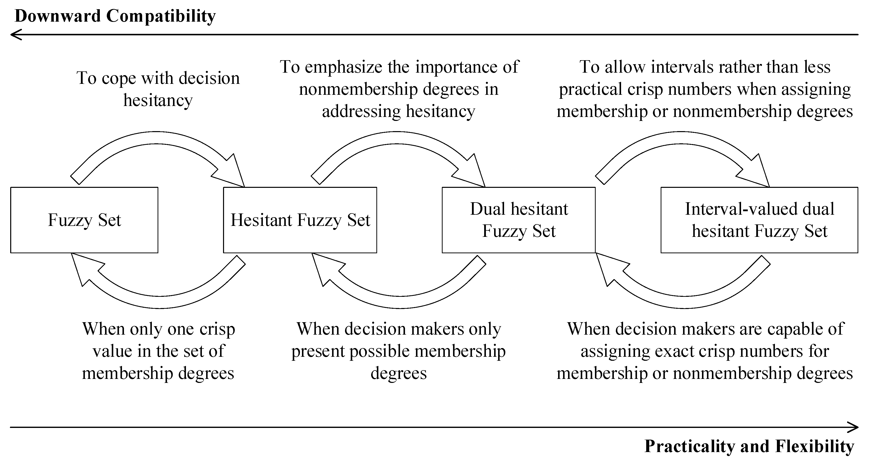Therefore, hesitant fuzzy set (HFS) [15,16] was recently put forward to address decision hesitancy in FMCGDM [20,21,22,23]. HFS only depicts decision hesitancy with possible membership degrees, while in fact non-membership degree plays the same important role as membership degree in describing fuzzy objects. Zhu, et al. [24] thus further defined dual hesitant fuzzy set (DHFS) to include both membership and non-membership. As pointed out in [25,26], DHFS can reflect decision hesitancy more completely than other extensions of FS. Subsequently, to accommodate decision settings of higher complexity (e.g., decision makers are only willing or able to give interval values rather than crisp ones because of time pressure or due to lack of expertise), Ju, et al. [27] and Farhadinia [25] introduced the interval-valued dual hesitant fuzzy set (IVDHFS). Thus far, only Ju, et al. [27] and Zhang, et al. [28] studied aggregation-operators-based models for multi-criteria decision making (MCDM) under interval-valued dual hesitant fuzzy (IVDHF) environments. Although their approaches can be extended to group settings, aggregation-operators-based models normally at least need to aggregate information twice [11,29], i.e., aggregate individual decision matrices into collective decision matrix, and then aggregate which to obtain final scores. Information loss increases with multiple use of aggregation operators [30], which also raises computational complexity especially for processing hesitant fuzzy preferences [31].

TOPSIS (Technique for Order Preference by Similarity to Ideal Solution) [32] and VIKOR (VlseKriterijuska Optimizacija I Komoromisno Resenje) [33,34] are two effective ideal-solution-based approaches for MCDM. TOPSIS maintains that the optimal alternative should have the shortest distance from the positive ideal solution and the farthest distance from the negative ideal solution, while VIKOR determines the compromise solution that is closest to the ideal solution and provides a minimum individual regret as well as a maximum group utility [34,35]. Mardani, et al. [12] and Kahraman, et al. [10] pointed out that TOPSIS and VIKOR have been adapted successfully to accommodate different fuzzy environments [36,37,38,39,40,41], but only few works were conducted on their extensions under hesitant fuzzy environments, such as those in [31,41,42,43,44,45,46]. To our best knowledge, scarcely any researchers have investigated TOPSIS and VIKOR for MCDM under interval-valued dual hesitant fuzzy (IVDHF) environments, much less in group settings. Therefore, in this paper, by employing IVDHFS to elicit decision makers’ hesitant preferences, we study effective FMCGDM approaches based on TOPSIS and VIKOR for tackling the complex ERSE problems, in which decision makers could be hesitant due to uncertainty and weighting information is totally unknown for both criteria and decision makers.

To do so, we first develop a deviation maximizing model to determine criteria weights and a compatibility maximizing program to derive weights for decision makers. Then, based on the determined weighting information, we propose two ideal-solution-based approaches for MCGDM with IVDHF preferences: IVDHF-TOPSIS and IVDHF-VIKOR. In IVDHF-TOPSIS, we utilize the obtained decision makers’ weights and the newly defined synthesized IVDHF group decision matrix to generate weighted group decision matrix so that IVDHF-TOPSIS can retain the straightforward ranking mechanism as in classical TOPSIS model by measuring distances from ideal solutions, instead of by employing aggregation operators. Aiming at supporting MCGDM under IVDHF environments where maximum group utility and minimum individual regret are required to be balanced, IVDHF-VIKOR firstly utilizes the derived decision makers’ weights to aggregate the individual decision matrix into group decision matrix, then extends the traditional VIKOR model to construct the compromised IVDHF ideal solution, and also incorporates the determined criteria weights in its ranking procedure to reflect relative importance of distances from the compromised IVDHF ideal solution.

The proposed IVDHF-TOPSIS and IVDHF-VIKOR hold the following main advantages: by employing IVDHFS to express decision hesitancy more comprehensively, they are more adequate and flexible for complex FMCGDM with hesitant preferences; they retain simple and straightforward decision procedures even in group decision making settings; in comparison with aggregation-operators-based approach, they can alleviate information loss and computational complexity caused by multiple use of aggregation operators (IVDHF-TOPSIS does not need any use of aggregation operators and IVDHF-VIKOR only requires an aggregation operator once to obtain group decision matrix).

The remainder of this paper is organized as follows. Based on IVDHFS, Section 2 gives the formulation for the emergency response solutions evaluation (ERSE) problems with consideration of decision hesitancy. In Section 3, optimization models are developed for obtaining weights for decision makers and criteria. Section 4 details two proposed approaches: IVDHF-TOPSIS and IVDHF-VIKOR. To validate the proposed approaches, we conduct numerical studies in Section 5. Finally, conclusions are made in Section 6.

2. Problem Formulation

2.1. Emergency Response Solutions Evaluation (ERSE)

Frequent happening of natural and man-made disaster catastrophic events has brought about huge impact on communities, families and many other societal units, not only suffering from illness or loss of lives but also from negative effects on economic and social conditions in the local area [6]. Lessons from these disasters have compelled governments to evaluate and include emergency response solutions regarding identifiable risks to guarantee sustainable community development. Although accumulated experiences can help local governments achieve a relative balance state of preparedness for specified risks by maintaining a set of effective response solutions, economic development programs launched in communities often break that balance and inevitably require local government to collect and evaluate emergency response solutions to cope with newly brought-in risks along with those programs. Besides the mentioned (in Section 1) emergency scenario that is threatening the YiWu International Trading Community, introducing novel technology-driven projects (such as nano-textiles, smart textiles, chemcial medicines, etc.) to unleash business opportunities in local communities has concurrently also brought about potential risks on environment, human health and safety, and sustainability (EHS/S) [47], which urges local governments to set up decision making procedures for emergency response solutions evalution (ERSE). Figure 1 depicts the basic motivation that ERSE has been recognized as a vital routine activity to serve emergency management in sustainable community planning [6,47,48].

Generally speaking, emergency response solution is a group of procedures to be implemented in case of a catastrophic event situation involving risk analysis, communication, intervention actions, operational support, logistic support, and whatever is necessary to reduce accident impacts [6,7,8,14,49]. Following suggestions of practices [50] and the lifecycle theory of emergency management [48,51], effective emergency response solutions should be prepared to cover three stages: pre-event, during-event and after-event. Correspondingly, when community development department (CDD) evaluates alternative emergency response solutions to potential risks of emergency scenarios, decision criteria should be derived from these three stages.

For another example, in many developing countries (such as China and other Asian countries) [52,53], increasing population and materials density due to continuous introduction of companies in certain industry clusters has made effective response solutions to urban fire accidents mandatory in sustainable community planning. When evaluating response solutions to urban fire accidents, according to lifecycle theory in emergency management, the following four indicators can be derived as main decision criteria [8,14,54,55].

(c₁) Accident identifying capacity, which comprehensively indicates the mature ability to utilize collected data in monitored control systems for early warning and the mature capacity of classifying accidents into different levels based on the obtained data and knowledge systems. It corresponds to the pre-event stage in the life cycle model of emergency management.

(c₂) Rescuing capacity, which indicates the rescuing action performance in the during-event stage of emergency management. It comprehensively reflects the completeness degree to which rescuing equipment and experienced rescue workers are prepared and how their commanding system is constructed.

(c₃) Emergency response resources supplying capacity, which not only requires provision of sufficient emergency resources, but also demands possession of relevant rescue technical knowledge and its decision support system. Overall, it indicates the competence of resources support function in response solutions for ensuring fulfillment of rescuing capacity in the during-event stage.

(c₄) After-accident management capacity, which is the capability of handling after-accident processing and resettlement requirements. A nexus of activities should be incorporated, such as tracking and feedback analyzing mechanism, knowledge bases, emergency policies for insurance services, and management systems for social donation. Generally, it assesses the maturity degree of management mechanisms for after-event processing work.

As we can see, this problem of emergency response solutions evaluation is characterized with both qualitative and quantitative assessment, obviously, it thus can be categorized as multi-criteria decision making (MCGDM) problems [8,14], that is, let $X=\{x_1,x_2,...,x_n\}$ be a set of emergency response solutions, $C=\{c_1,c_2,...,c_m\}$ be the set of criteria. Define $D=\{d_1,d_2,...,d_t\}$ as the decision makers in an evaluation team responsible for the evaluation of all solutions $X=\{x_1,x_2,...,x_n\}$. Then, after each decision maker assess the scores of solution $x_i\left(i=1,\mathrm{...},n\right)$ under criterion $c_j\left(j=1,\mathrm{...},m\right)$, we can obtain the following decision matrix $R^k={(r_{ij})}_{m\times n}$ as

Rk		Criteria
		$c_1$	$c_2$	…	$c_m$
Solutions	$x_1$	$r_{11}^k$	$r_{12}^k$	…	$r_{1m}^k$
	$x_2$	$r_{21}^k$	$r_{22}^k$	…	$r_{2m}^k$
	$⋮$	$⋮$	$⋮$	$⋮$	$⋮$
	$x_n$	$r_{n1}^k$	$r_{n2}^k$	…	$r_{nm}^k$

Here preferences ${(r_{ij})}_{m\times n}$ usually is represented by using exact values and the purpose of the evaluation activity is to derive the most appropriate one(s) based on information in decision matrix $R^k={(r_{ij})}_{m\times n}$. However, due to the complexity and uncertainty in emergency response solutions evaluation, decision makers are often hesitant or irresolute with expressing their assessments. Therefore, appropriate representation tools should be introduced to effectively incorporate decision maker’s preferences with hesitancy [16].

2.2. Interval-Valued Dual Hesitant Fuzzy Representation Approach

In order to help decision makers express their uncertain preferences, Zadeh [56] firstly introduced the fuzzy set (FS) theory as a quantitative tool for decision making under uncertainty. Since its appearance, FS has been successfully applied to multi-criteria decision making [10,12], and its extensions have also been investigation in-depth to elicit uncertain decision preferences more effectively and comprehensively, such as interval-valued fuzzy set [57], intuitionistic fuzzy set (IFS) [58], interval-valued intuitionistic fuzzy set [59]. However, these fuzzy representation approaches are generally not suitable for situations where decision makers are hesitant or irresolute in describing membership degrees to a fuzzy concept because of several possible values, so Torra [16], Torra and Narukawa [15] defined hesitant fuzzy set (HFS) to allow membership degrees of an element to be a set of values. For example, decision makers are allowed to express their preference with <c_i, (0.3, 0.4, 0.5)>, which means 0.3, 0.4, 0.5 are the possible membership degrees to which an alternative solution satisfying criterion c_i. HFS are highly useful in handling complex situations with decision hesitance [60,61]. Inspired by the fundamental ideas in HFS and IFS, Zhu, et al. [24] further developed the dual hesitant fuzzy set (DHFS) to allow both hesitant membership and non-membership degrees of an element to a given concept by using two sets of crisp values. Then, to be more applicable as suggested in [59], Ju, et al. [27], and Farhadinia [25] studied DHFS under interval-valued environments and provide the more flexible representation model: interval-valued dual hesitant fuzzy set (IVDHFS). Relations between all above-mentioned representation models are depicted in Figure 2. Evidently, IVDHFS is more practical in multi-criteria decision making for the reason that it provides an effective and flexible way to assign values for each element in the domains [25,26]. Therefore, in this paper, we employ IVDHFS to help decision makers elicit their preferences more effectively and comprehensively in emergency response solutions evaluation.

In the following, basic notions, distance measures, and aggregation operators for IVDHFS are introduced.

2.2.1. Interval-Valued Dual Hesitant Fuzzy Set (IVDHFS)

Definition 2.1. [16]. Let $X$ be a fixed set. A HFS in $X$ is defined a function E that when applied to $X$ returns a subset of $[0,1]$. It can be expressed as

$$E=\left\{\langle x,h_E(x)\rangle |x\in X\right\}$$

(1)

where $h_E(x)$ is a set of values in $[0,1]$, denoting possible membership degrees of the element $x\in X$ to the set $E$.

HFS in [16] only addresses possible membership degrees of an element to a given set without considering non-membership degrees. To overcome this limitation, Zhu, et al. [24] proposed the dual hesitant fuzzy sets (DHFS):

Definition 2.2. [24]. Let $X$ be a fixed set, then a dual hesitant fuzzy set (DHFS) on $X$ can be defined as:

$$D=\left\{\langle x,h(x),g(x)\rangle |x\in X\right\}$$

(2)

where $h(x)={\displaystyle {\cup }_{\mu \in h(x)}\left\{\mu \right\}}$ and $g(x)={\displaystyle {\cup }_{\nu \in g(x)}\left\{\nu \right\}}$ are two sets of values in $[0,1]$, respectively denoting possible membership degrees and non-membership degrees of an element $x\in X$ to the set $D$, which requires the conditions: $\mu ,\nu \in [0,1]$, $0\le {\mu }^{+}+{\nu }^{+}\le 1$, where $\mu \in h(x)$, $\nu \in g(x)$, ${\mu }^{+}\in h^{+}(x)={\displaystyle {\cup }_{\mu \in h(x)}\max \left\{\mu \right\}}$ and ${\nu }^{+}\in g^{+}(x)={\displaystyle {\cup }_{\nu \in g(x)}\max \left\{\nu \right\}}$ for all $x\in X$.

$d=(h,g)$ is called a dual hesitant fuzzy element (DHFE) and $D$ is the set of all DHFEs.

However, the precise membership degrees and non-membership degrees of an element to a set are sometimes hard to determine. To overcome this barrier, Ju, et al. [27] and Farhadinia [25] introduced the following effective tool of interval-valued dual hesitant fuzzy set (IVDHFS).

Definition 2.3. [25,27]. Let $X$ be a fixed set, then an IVDHFS on $X$ can be defined as:

$$\tilde{D}=\left\{\langle x,\tilde{h}(x),\tilde{g}(x)\rangle |x\in X\right\}$$

(3)

where $\tilde{h}(x)={\displaystyle {\cup }_{[{\mu }^L,{\mu }^U]\in \tilde{h}(x)}\left\{\tilde{\mu }\right\}}={\displaystyle {\cup }_{[{\mu }^L,{\mu }^U]\in \tilde{h}(x)}\{[{\mu }^L,{\mu }^U]\}}$ and $\tilde{g}(x)={\displaystyle {\cup }_{[{\nu }^L,{\nu }^U]\in \tilde{g}(x)}\left\{\tilde{\nu }\right\}}={\displaystyle {\cup }_{[{\nu }^L,{\nu }^U]\in \tilde{g}(x)}\{[{\nu }^L,{\nu }^U]\}}$ are two sets of interval values in $[0,1]$, which respectively denote possible membership and non-membership degrees of element $x\in X$ to the set $\tilde{D}$. $\tilde{\mu }$ and $\tilde{\nu }$ hold conditions: $\tilde{\mu },\tilde{\nu }\in [0,1]$, $0\le {({\mu }^U)}^{+}+{({\nu }^U)}^{+}\le 1$, where ${({\mu }^U)}^{+}\in {\tilde{h}}^{+}(x)={\displaystyle {\cup }_{[{\mu }^L,{\mu }^U]\in \tilde{h}(x)}\max \left\{{\mu }^U\right\}}$ and ${({\nu }^U)}^{+}\in {\tilde{g}}^{+}(x)={\displaystyle {\cup }_{[{\nu }^L,{\nu }^U]\in \tilde{g}(x)}\max \left\{{\nu }^U\right\}}$ for $x\in X$.

Usually, $\tilde{d}=(\tilde{h},\tilde{g})$ is called an IVDHF element (IVDHFE) and $\tilde{D}$ is the set of all IVDHFEs. And the following Definitions 2.4 and 2.5 give the fundamental operations for IVDHFEs.

Definition 2.4. [27]. Given three IVDHFEs: $\tilde{d}=(\tilde{h},\tilde{g})$, ${\tilde{d}}_1=({\tilde{h}}_1,{\tilde{g}}_1)$, ${\tilde{d}}_2=({\tilde{h}}_2,{\tilde{g}}_2)$, then some of the important operations relationships can be described below:

(1)

${\tilde{d}}^{\lambda }={\displaystyle {\cup }_{[{\mu }^L,{\mu }^U]\in \tilde{h},[{\nu }^L,{\nu }^U]\in \tilde{g}}\left\{\right\{[{({\mu }^L)}^{\lambda },{({\mu }^U)}^{\lambda }]\},\{[1-{(1-{\nu }^L)}^{\lambda },1-{(1-{\nu }^U)}^{\lambda }]\left\}\right\}}$, $\lambda >0$;

(2)

$\lambda \tilde{d}={\displaystyle {\cup }_{[{\mu }^L,{\mu }^U]\in \tilde{h},[{\nu }^L,{\nu }^U]\in \tilde{g}}\left\{\right\{[1-{(1-{\mu }^L)}^{\lambda },1-{(1-{\mu }^U)}^{\lambda }]\},\{[{({\nu }^L)}^{\lambda },{({\nu }^U)}^{\lambda }]\left\}\right\}}$, $\lambda >0$;

(3)

${\tilde{d}}_1\oplus {\tilde{d}}_2={\displaystyle {\cup }_{[{\mu }_1^L,{\mu }_1^U]\in {\tilde{h}}_1,[{\mu }_2^L,{\mu }_2^U]\in {\tilde{h}}_2,[{\nu }_1^L,{\nu }_1^U]\in {\tilde{g}}_1,[{\nu }_2^L,{\nu }_2^U]\in {\tilde{g}}_2}\left\{\right\{[{\mu }_1^L+{\mu }_2^L-{\mu }_1^L{\mu }_2^L,{\mu }_1^U+{\mu }_2^U-{\mu }_1^U{\mu }_2^U]\},\{[{\nu }_1^L{\nu }_2^L,{\nu }_1^U{\nu }_2^U]\left\}\right\}}$;

(4)

${\tilde{d}}_1\otimes {\tilde{d}}_2={\displaystyle {\cup }_{[{\mu }_1^L,{\mu }_1^U]\in {\tilde{h}}_1,[{\mu }_2^L,{\mu }_2^U]\in {\tilde{h}}_2,[{\nu }_1^L,{\nu }_1^U]\in {\tilde{g}}_1,[{\nu }_2^L,{\nu }_2^U]\in {\tilde{g}}_2}\left\{\right\{[{\mu }_1^L{\mu }_2^L,{\mu }_1^U{\mu }_2^U]\},\{[{\nu }_1^L+{\nu }_2^L-{\nu }_1^L{\nu }_2^L,{\nu }_1^U+{\nu }_2^U-{\nu }_1^U{\nu }_2^U]\left\}\right\}}$.

Definition 2.5. [27]. Let ${\tilde{d}}_1=({\tilde{h}}_1,{\tilde{g}}_1)$ and ${\tilde{d}}_2=({\tilde{h}}_2,{\tilde{g}}_2)$ be any two IVDHFEs, then some operation rules can be defined as:

(1)

${\tilde{d}}_1\oplus {\tilde{d}}_2={\tilde{d}}_2\oplus {\tilde{d}}_1$;

(2)

${\tilde{d}}_1\otimes {\tilde{d}}_2={\tilde{d}}_2\otimes {\tilde{d}}_1$;

(3)

$\lambda ({\tilde{d}}_1\oplus {\tilde{d}}_2)=\lambda {\tilde{d}}_1\oplus \lambda {\tilde{d}}_2$, $\lambda >0$;

(4)

${\tilde{d}}_1^{\lambda }\otimes {\tilde{d}}_2^{\lambda }={({\tilde{d}}_2\otimes {\tilde{d}}_1)}^{\lambda }$, $\lambda >0$.

In Ju, et al. [27], they also introduced a score function $S(\tilde{d})$ to compute scores of $\tilde{d}$, and defined an accuracy function $P(\tilde{d})$ to evaluate the accuracy degrees of $\tilde{d}$, where

$$S(\tilde{d})=\frac{1}{2}\left(\frac{1}{l(\tilde{h})}{\displaystyle {\sum }_{[{\mu }^L,{\mu }^U]\in \tilde{h}}{\mu }^L}-\frac{1}{l(\tilde{g})}{\displaystyle {\sum }_{[{\nu }^L,{\nu }^U]\in \tilde{g}}{\nu }^L}+\frac{1}{l(\tilde{h})}{\displaystyle {\sum }_{[{\mu }^L,{\mu }^U]\in \tilde{h}}{\mu }^U}-\frac{1}{l(\tilde{g})}{\displaystyle {\sum }_{[{\nu }^L,{\nu }^U]\in \tilde{g}}{\nu }^U}\right),$$

(4)

$$P(\tilde{d})=\frac{1}{2}\left(\frac{1}{l(\tilde{h})}{\displaystyle {\sum }_{[{\mu }^L,{\mu }^U]\in \tilde{h}}{\mu }^L}+\frac{1}{l(\tilde{g})}{\displaystyle {\sum }_{[{\nu }^L,{\nu }^U]\in \tilde{g}}{\nu }^L}+\frac{1}{l(\tilde{h})}{\displaystyle {\sum }_{[{\mu }^L,{\mu }^U]\in \tilde{h}}{\mu }^U}+\frac{1}{l(\tilde{g})}{\displaystyle {\sum }_{[{\nu }^L,{\nu }^U]\in \tilde{g}}{\nu }^U}\right),$$

(5)

and $l(\tilde{h})$, $l(\tilde{g})$ are the numbers of interval values in $\tilde{h}$ and $\tilde{g}$, respectively. The larger the score $S(\tilde{d})$, the larger the accuracy $P(\tilde{d})$, and the greater the IVDHFE $\tilde{d}$.

Then order relations between any two IVDHFEs ${\tilde{d}}_1=({\tilde{h}}_1,{\tilde{g}}_1)$, ${\tilde{d}}_2=({\tilde{h}}_2,{\tilde{g}}_2)$ can be determined according to the following rules:

• If $S({\tilde{d}}_1)<S({\tilde{d}}_2)$, then ${\tilde{d}}_1<{\tilde{d}}_2$.
• If $S({\tilde{d}}_1)=S({\tilde{d}}_2)$, then (1) If $P({\tilde{d}}_1)=P({\tilde{d}}_2)$, then ${\tilde{d}}_1={\tilde{d}}_2$; (2) If $P({\tilde{d}}_1)<P({\tilde{d}}_2)$, then ${\tilde{d}}_1<{\tilde{d}}_2$.

2.2.2. Distance Measures for IVDHFS

In order to calculate the distance between any two IVDHFEs, we utilize the complementing method introduced by Xu and Xia [62] to extend IVDHFE’s membership set or non-membership set which hold smaller cardinality. That is, given any two IVDHFEs:

$${\tilde{d}}_1=({\tilde{h}}_1,{\tilde{g}}_1)=\left({\displaystyle {\cup }_{[{\mu }_1^L,{\mu }_1^L]\in {\tilde{h}}_1}\{[{\mu }_1^L,{\mu }_1^U]\}},{\displaystyle {\cup }_{[{\nu }_1^L,{\nu }_1^L]\in {\tilde{g}}_1}\{[{\nu }_1^L,{\nu }_1^U]\}}\right)$$

and

$${\tilde{d}}_2=({\tilde{h}}_2,{\tilde{g}}_2)=\left({\displaystyle {\cup }_{[{\mu }_2^L,{\mu }_2^L]\in {\tilde{h}}_2}\{[{\mu }_2^L,{\mu }_2^U]\}},{\displaystyle {\cup }_{[{\nu }_2^L,{\nu }_2^L]\in {\tilde{g}}_2}\{[{\nu }_2^L,{\nu }_2^U]\}}\right),$$

where $l_{{\tilde{h}}_1}$ and $l_{{\tilde{h}}_2}$ are the numbers of elements in ${\tilde{h}}_1$ and ${\tilde{h}}_2$, $l_{{\tilde{g}}_1}$ and $l_{{\tilde{g}}_2}$ are the numbers of elements in ${\tilde{g}}_1$ and ${\tilde{g}}_2$. Usually there exist $l_{{\tilde{h}}_1}\ne l_{{\tilde{h}}_2}$ and $l_{{\tilde{g}}_1}\ne l_{{\tilde{g}}_2}$, under such cases we can, as suggested by Xu and Xia [62], extend every set with smaller cardinality by adding values according to certain principle so as to meet conditions: $l_{\tilde{h}}=\max \{l_{{\tilde{h}}_1},l_{{\tilde{h}}_2}\}$, $l_{\tilde{g}}=\max \{l_{{\tilde{g}}_1},l_{{\tilde{g}}_2}\}$.

In this paper, we adopt the complementing method with pessimistic decision principle to derive the following normalized Euclidean distance for IVDHFEs.

Definition 2.6. Let ${\tilde{d}}_1$ and ${\tilde{d}}_2$ be two IVDHFEs, then the normalized Euclidean distance for IVDHFEs can be defined as

$$\begin{array}{cc}{d}_{IVDHFS}({\tilde{d}}_1,{\tilde{d}}_2)& =(\frac{1}{2}(\frac{1}{l_{\tilde{h}}}{\displaystyle {\sum }_{j=1}^{l_{\tilde{h}}}\left({\left|{\mu }_{{\tilde{h}}_1}^{L_{\sigma (j)}}-{\mu }_{{\tilde{h}}_2}^{L_{\sigma (j)}}\right|}^2+{\left|{\mu }_{{\tilde{h}}_1}^{U_{\sigma (j)}}-{\mu }_{{\tilde{h}}_2}^{U_{\sigma (j)}}\right|}^2\right)}\\ & {+\frac{1}{l_{\tilde{g}}}{\displaystyle {\sum }_{j=1}^{l_{\tilde{g}}}\left({\left|{\nu }_{{\tilde{g}}_1}^{L_{\sigma (j)}}-{\nu }_{{\tilde{g}}_2}^{L_{\sigma (j)}}\right|}^2+{\left|{\nu }_{{\tilde{g}}_1}^{U_{\sigma (j)}}-{\nu }_{{\tilde{g}}_2}^{U_{\sigma (j)}}\right|}^2\right)}))}^{\raisebox{1ex}{$1$}\!\left/ \!\raisebox{-1ex}{$2$}\right.},\end{array}$$

(6)

where ${\mu }_{{\tilde{h}}_1}^{L_{\sigma (j)}}$, ${\mu }_{{\tilde{h}}_2}^{L_{\sigma (j)}}$, ${\mu }_{{\tilde{h}}_1}^{U_{\sigma (j)}}$ and ${\mu }_{{\tilde{h}}_2}^{U_{\sigma (j)}}$ are the $j$ th largest lower and upper values in ${\tilde{h}}_1$ and ${\tilde{h}}_2$ respectively, while ${\nu }_{{\tilde{h}}_1}^{L_{\sigma (j)}}$, ${\nu }_{{\tilde{h}}_2}^{L_{\sigma (j)}}$, ${\nu }_{{\tilde{h}}_1}^{U_{\sigma (j)}}$ and ${\nu }_{{\tilde{h}}_2}^{U_{\sigma (j)}}$ are the $j$ th largest lower and upper values in ${\tilde{g}}_1$ and ${\tilde{g}}_2$ respectively.

For the above Euclidean distance measure $d_{IVDHFS}$, we have the following theorem.

Theorem 2.1. 

The Euclidean distance measure $d_{IVDHFS}$ satisfies properties:

(1)

$0\le d_{IVDHFS}({\tilde{d}}_1,{\tilde{d}}_2)\le 1$;

(2)

$d_{IVDHFS}({\tilde{d}}_1,{\tilde{d}}_2)=0$ if and only if ${\tilde{d}}_1$ and ${\tilde{d}}_2$ are perfectly consistent;

(3)

$d_{IVDHFS}({\tilde{d}}_1,{\tilde{d}}_2)=d_{IVDHFS}({\tilde{d}}_2,{\tilde{d}}_1)$.

2.2.3. Basic Aggregation Operators for IVDHFS

Definition 2.7. [27]. For a collection of IVDHFEs ${\tilde{d}}_j(j=1,2,...,n)$, an IVDHF weighted average (IVDHFWA) operator is a mapping of $S^n\to S$, such that

$$\begin{array}{c}IVDHFW{A}_{\omega }({\tilde{d}}_1,{\tilde{d}}_2,...,{\tilde{d}}_n)=\underset{j=1}{\overset{n}{\oplus }}({\omega }_j{\tilde{d}}_j)\\ ={\cup }_{[{\mu }_j^L,{\mu }_j^U]\in {\tilde{h}}_j,[{\nu }_j^L,{\nu }_j^U]\in {\tilde{g}}_j}\left\{\left\{\left[1-{\displaystyle \prod _{j=1}^n{(1-{\mu }_j^L)}^{{\omega }_j}},1-{\displaystyle \prod _{j=1}^n{(1-{\mu }_j^U)}^{{\omega }_j}}\right]\right\},\left\{\left[{\displaystyle \prod _{j=1}^n{({\nu }_j^L)}^{{\omega }_j}},{\displaystyle \prod _{j=1}^n{({\nu }_j^U)}^{{\omega }_j}}\right]\right\}\right\},\end{array}$$

(7)

where $\omega ={({\omega }_1,{\omega }_2,...,{\omega }_n)}^T$ is the weighting vector for ${\tilde{d}}_j(j=1,2,...,n)$, ${\omega }_j\in [0,1]$ and ${\displaystyle {\sum }_{j=1}^n{\omega }_j}=1.$

Definition 2.8. [27]. For a collection of IVDHFEs ${\tilde{d}}_j(j=1,2,...,n)$, an IVDHF weighted geometric average (IVDHFWGA) operator is a mapping of $S^n\to S$ such that

$$\begin{array}{c}IVDHFWG{A}_{\omega }({\tilde{d}}_1,{\tilde{d}}_2,...,{\tilde{d}}_n)=\underset{j=1}{\overset{n}{\otimes }}{({\tilde{d}}_j)}^{{\omega }_j}\\ ={\cup }_{[{\mu }_j^L,{\mu }_j^U]\in {\tilde{h}}_j,[{\nu }_j^L,{\nu }_j^U]\in {\tilde{g}}_j}\left\{\left\{\left[{\displaystyle \prod _{j=1}^n{({\mu }_j^L)}^{{\omega }_j}},{\displaystyle \prod _{j=1}^n{({\mu }_j^U)}^{{\omega }_j}}\right]\right\},\left\{\left[1-{\displaystyle \prod _{j=1}^n{(1-{\nu }_j^L)}^{{\omega }_j}},1-{\displaystyle \prod _{j=1}^n{(1-{\nu }_j^U)}^{{\omega }_j}}\right]\right\}\right\},\end{array}$$

(8)

where $\omega ={({\omega }_1,{\omega }_2,...,{\omega }_n)}^T$ is the weighting vector of ${\tilde{d}}_j(j=1,2,...,n)$, ${\omega }_j\in [0,1]$ and ${\displaystyle {\sum }_{j=1}^n{\omega }_j}=1$.

2.3. Problem Formulation of ERSE with Interval-Valued Dual Hesitant Fuzzy Preferences

Now, in the case in that decision makers are hesitant with assessments due to problem complexity and time pressure [16], we empower decision makers to express their hesitant preferences based on the above-discussed IVDHFS during the solving process of ERSE.

That is, we can reconsider the ERSE as a type of FMCGDM problems under interval-valued dual hesitant fuzzy environments: suppose $X=\{x_1,x_2,...,x_n\}$ be a set of emergency response solutions; $C=\{c_1,c_2,...,c_m\}$ be the set of criteria, $\omega ={({\omega }_1,{\omega }_2,...,{\omega }_m)}^T$ is the weighting vector for criteria $c_j$, where ${\omega }_j\ge 0$, $j=1,2,...,m$ and ${\displaystyle {\sum }_{j=1}^m{\omega }_j}=1$; denote $D=\{d_1,d_2,...,d_t\}$ as a finite set of decision makers that are responsible for the assessment of all solutions, and $\lambda =({\lambda }_1,{\lambda }_2,...,{\lambda }_t)$ as their weighting vector, where ${\lambda }_k\ge 0(k=1,2,...,t)$ and ${\displaystyle {\sum }_{k=1}^t{\lambda }_k}=1$. Then, after collecting the assessments provided by all decision makers, we can obtain the decision matrices ${\tilde{R}}^k={({\tilde{r}}_{ij}^k)}_{n\times m}(i=1,2,...,n;j=1,2,...,m;k=1,2,...,t)$ that take the form shown in

Table 1. Interval-valued dual hesitant fuzzy decision matrix given by the k-th decision maker.

${\tilde{R}}^k$ (Unknown Expert Weighting Vector $\lambda$)		Criteria (Unknown Criteria Weighting Vector $\omega$)
		$c_1$	$c_2$	…	$c_m$
Emergency Response Solutions	$x_1$	${\tilde{r}}_{11}^k=({\tilde{h}}_{11}^k,{\tilde{g}}_{11}^k)$	${\tilde{r}}_{12}^k=({\tilde{h}}_{12}^k,{\tilde{g}}_{12}^k)$	…	${\tilde{r}}_{1m}^k=({\tilde{h}}_{1m}^k,{\tilde{g}}_{1m}^k)$
	$x_2$	${\tilde{r}}_{21}^k=({\tilde{h}}_{21}^k,{\tilde{g}}_{21}^k)$	${\tilde{r}}_{22}^k=({\tilde{h}}_{22}^k,{\tilde{g}}_{22}^k)$	…	${\tilde{r}}_{2m}^k=({\tilde{h}}_{2m}^k,{\tilde{g}}_{2m}^k)$
	$⋮$	$⋮$	$⋮$	$⋮$	$⋮$
	$x_n$	${\tilde{r}}_{n1}^k=({\tilde{h}}_{n1}^k,{\tilde{g}}_{n1}^k)$	${\tilde{r}}_{n2}^k=({\tilde{h}}_{n2}^k,{\tilde{g}}_{n2}^k)$	…	${\tilde{r}}_{nm}^k=({\tilde{h}}_{nm}^k,{\tilde{g}}_{nm}^k)$

.

In Table 1, ${\tilde{r}}_{ij}^k=({\tilde{h}}_{ij}^k,{\tilde{g}}_{ij}^k)$ is an IVDHFE representing the assessments of the alternative $x_i$ with respect to the criterion $c_j$. ${\tilde{h}}_{ij}^k$ indicates all possible membership degrees that alternative $x_i$ satisfy criterion $c_j$, while ${\tilde{g}}_{ij}^k$ indicates all possible non-membership degrees that alternative $x_i$ does not satisfy criterion $c_j$.

Additionally, without loss of generality, since decision makers are chosen from different backgrounds with specific expertise, equal weights or other arbitrary weights should not be directly assigned to decision makers either [63]. On the other hand, also due to the problem complexity or time pressure, criteria weights often cannot be determined with empirical values appropriately in advance [11,64]. Consequently, for the FMCGDM problem of ERSE under discussion, the criteria weighting vector $\omega$ and decision makers’ weighting vector $\lambda$ are treated as unknown and to be determined.

In order to construct effective FMCGDM approaches for tackling the above ERSE problems, in the following Section 3, we focus on optimization models based on the obtained decision matrices for objectively determining $\omega$ and $\lambda$ since they should not be allocated subjectively.

3. Optimization Models for Obtaining Unknown Weights for Criteria and Decision Makers

When weights for criteria and decision makers cannot be determined appropriately in advance, they can be objectively derived from preferences provided by decision makers [63,65]. Based on decision information provided in the form of IVDHFS, we propose a compatibility maximizing model to obtain weights for decision makers, and another deviation maximizing model to determine weights for criteria.

3.1. Compatibility Maximizing Model for Deriving Weights for Decision Makers

Similarity measure, a straightforward procedure for consensus degree, has been successfully employed to differentiate decision makers [66,67]. The main idea of similarity measure based differentiation is that: the smaller the difference between an expert’s decision matrix and the ones offered by other decision makers, the more precise the information provided by the expert, thus a larger weight should be assigned to this expert. Borrowing this idea, in what follows, we first define the compatibility degree based on divergence between any two IVDHF decision matrices; then, we propose a compatibility maximizing model to obtain optimum weighting vector for all decision makers.

Based on Definition 2.6, we can obtain the following definition of compatibility degree.

Definition 3.1. Let ${\tilde{R}}^1={({\tilde{r}}_{ij}^1)}_{n\times m}$, ${\tilde{R}}^2={({\tilde{r}}_{ij}^2)}_{n\times m}$ be any two IVDHF decision matrices as the same form shown in Table 1. Then, the compatibility degree CI between ${\tilde{R}}^1$ and ${\tilde{R}}^2$ can be defined as

$$CI({\tilde{R}}^1,{\tilde{R}}^2)=1-\frac{1}{nm}{\displaystyle {\sum }_{i=1}^n{\displaystyle {\sum }_{j=1}^m{d}_{IVDHFS}({\tilde{r}}_{ij}^1,{\tilde{r}}_{ij}^2)}},$$

(9)

where $d_{IVDHFS}$ is the distance measure introduced in Definition 2.6. Obviously, $CI({\tilde{R}}^1,{\tilde{R}}^2)$ is the sum of compatibility degree of all the corresponding IVDHFEs from ${\tilde{R}}^1$ and ${\tilde{R}}^2$. Thereby, it can reflect total divergence between matrices ${\tilde{R}}^1$ and ${\tilde{R}}^2$. Note that the compatibility degree is non-negative and commutative.

In addition, we have the following theorem for the compatibility degree $CI$.

Theorem 3.1. 

Suppose ${\tilde{R}}^1={({\tilde{r}}_{ij}^1)}_{n\times m}$ and ${\tilde{R}}^2={({\tilde{r}}_{ij}^2)}_{n\times m}$ are two IVDHF decision matrices, then

(1)

$0\le CI({\tilde{R}}^1,{\tilde{R}}^2)\le 1$;

(2)

$CI({\tilde{R}}^1,{\tilde{R}}^2)=1$ if and only if ${\tilde{R}}^1$ and ${\tilde{R}}^2$ are perfectly consistent;

(3)

$CI({\tilde{R}}^1,{\tilde{R}}^2)=CI({\tilde{R}}^2,{\tilde{R}}^1)$.

Proof. 

(1)

$CI({\tilde{R}}^1,{\tilde{R}}^2)=1-\frac{1}{nm}{\displaystyle {\sum }_{i=1}^n{\displaystyle {\sum }_{j=1}^m{d}_{IVDHFS}({\tilde{r}}_{ij}^1,{\tilde{r}}_{ij}^2)}}\ge 0$;

(2)

If $CI({\tilde{R}}^1,{\tilde{R}}^2)=1$, then $d_{IVDHFS}({\tilde{r}}_{ij}^1,{\tilde{r}}_{ij}^2)=0$. Then, ${\tilde{r}}_{ij}^1={\tilde{r}}_{ij}^2$, ${\tilde{R}}^1$ and ${\tilde{R}}^2$ are perfectly consistent;

If ${\tilde{R}}^1$ and ${\tilde{R}}^2$ are perfectly consistent, then $d_{IVDHFS}({\tilde{r}}_{ij}^1,{\tilde{r}}_{ij}^2)=0$. Thus, we have ${\tilde{r}}_{ij}^1={\tilde{r}}_{ij}^2$ and $CI({\tilde{R}}^1,{\tilde{R}}^2)=1$;

(3)

Note that compatibility degree $CI$ is based on the distance measure $d_{IVDHFS}$ between two IVDHFEs, where $d_{IVDHFS}$ holds the property of commutativity. Therefore we have

$$\begin{array}{cc}CI({\tilde{R}}^1,{\tilde{R}}^2)& =1-\frac{1}{nm}{\displaystyle {\sum }_{i=1}^n{\displaystyle {\sum }_{j=1}^m{d}_{IVDHFS}({\tilde{r}}_{ij}^1,{\tilde{r}}_{ij}^2)}}\hfill \\ & =1-\frac{1}{nm}{\displaystyle {\sum }_{i=1}^n{\displaystyle {\sum }_{j=1}^m{d}_{IVDHFS}({\tilde{r}}_{ij}^2,{\tilde{r}}_{ij}^1)}}\hfill \\ & =CI({\tilde{R}}^2,{\tilde{R}}^1),\hfill \end{array}$$

which completes the proof. □

Now, based on the above compatibility degree, we can differentiate decision makers. Namely, if the total divergence of ${\tilde{R}}^k$ (given by the kth decision maker) from other decision matrices appears to be larger than other decision matrices’ divergences, then the kth decision maker plays a less important role in decision making and should be assigned a smaller weight. On the contrary, a small overall divergence score suggests the kth decision maker plays an important role in prioritization process and should be assigned a bigger weight. Thereby, a compatibility maximizing model can be constructed to obtain optimum expert weights as following

$$(M-0)\{\begin{array}{l}\max F({\lambda }_k)={\displaystyle \sum _{k=1}^t\left(\frac{1}{t-1}{\displaystyle \sum _{l=1,l\ne k}^{t}CI({\tilde{R}}^k,{\tilde{R}}^l)}\right){\lambda }_k}\\ s.t{\displaystyle \sum _{k=1}^t{\lambda }_k{}^2}=1,{\lambda }_k\ge 0,k=1,2,...,t\end{array}.$$

For more clarity, we can rewrite (M-0) as

$$(M-1)\{\begin{array}{l}\max F({\lambda }_k)={\displaystyle \sum _{k=1}^t\left(\frac{1}{t-1}{\displaystyle \sum _{l=1,l\ne k}^t(1-\frac{1}{nm}{\displaystyle {\sum }_{i=1}^n{\displaystyle {\sum }_{j=1}^m{d}_{IVDHFS}({\tilde{r}}_{ij}^k,{\tilde{r}}_{ij}^l)}}}\right){\lambda }_k}\\ s.t{\displaystyle \sum _{k=1}^t{\lambda }_k{}^2}=1,{\lambda }_k\ge 0,k=1,2,...,t\end{array}.$$

For model (M-1), we have the following theorem.

Theorem 3.2. 

The optimal solution to model (M-1) is

$${\lambda }_k=\frac{{\displaystyle {\sum }_{l=1,l\ne k}^t\left(1-\frac{1}{nm}{\displaystyle {\sum }_{i=1}^n{\displaystyle {\sum }_{j=1}^m{d}_{IVDHFS}({\tilde{r}}_{ij}^k,{\tilde{r}}_{ij}^l)}}\right)}}{{\displaystyle {\sum }_{k=1}^t{\displaystyle {\sum }_{l=1,l\ne k}^t\left(1-\frac{1}{nm}{\displaystyle {\sum }_{i=1}^n{\displaystyle {\sum }_{j=1}^m{d}_{IVDHFS}({\tilde{r}}_{ij}^k,{\tilde{r}}_{ij}^l)}}\right)}}}$$

(10)

Proof. 

Regarding the model (M-1), we can apply the Lagrange Multiplier Method to derive its optimal solution.

To begin with the deduction, we first construct the following Lagrange function

$$L({\lambda }_k,\zeta )={\displaystyle \sum _{k=1}^t\left(\frac{1}{t-1}{\displaystyle \sum _{l=1,l\ne k}^t(1-\frac{1}{nm}{\displaystyle {\sum }_{i=1}^n{\displaystyle {\sum }_{j=1}^m{d}_{IVDHFS}({\tilde{r}}_{ij}^k,{\tilde{r}}_{ij}^l)}}}\right){\lambda }_k}+\frac{1}{2}\zeta {\displaystyle \sum _{k=1}^t({\lambda }_k{}^2-1)}.$$

(11)

Then, differentiate Equation (11) with respect to ${\lambda }_k$ and $\zeta$. Set these partial derivatives equal to 0, we have:

$$\{\begin{array}{l}\frac{\partial L}{\partial {\lambda }_k}=\frac{1}{t-1}{\displaystyle \sum _{l=1,l\ne k}^t(1-\frac{1}{nm}{\displaystyle {\sum }_{i=1}^n{\displaystyle {\sum }_{j=1}^m{d}_{IVDHFS}({\tilde{r}}_{ij}^k,{\tilde{r}}_{ij}^l)}}}+\zeta {\lambda }_k=0\\ \frac{\partial L}{\partial \zeta }={\displaystyle \sum _{k=1}^t({\lambda }_k{}^2-1)}=0\end{array}$$

(12)

After solving Equation (12), we attain the weights for the kth decision maker as follows,

$${\lambda }_k=\frac{\frac{1}{t-1}{\displaystyle {\sum }_{l=1,l\ne k}^t(1-\frac{1}{nm}{\displaystyle {\sum }_{i=1}^n{\displaystyle {\sum }_{j=1}^m{d}_{IVDHFS}({\tilde{r}}_{ij}^k,{\tilde{r}}_{ij}^l)}}}}{\sqrt{{\displaystyle {\sum }_{k=1}^t{(\frac{1}{t-1}{\displaystyle {\sum }_{l=1,l\ne k}^t(1-\frac{1}{nm}{\displaystyle {\sum }_{i=1}^n{\displaystyle {\sum }_{j=1}^m{d}_{IVDHFS}({\tilde{r}}_{ij}^k,{\tilde{r}}_{ij}^l)}}})}^2}}}\mathrm{.}$$

(13)

By normalizing ${\lambda }_k(k=1,2,...,t)$, we have the optimal solution:

$${\lambda }_k=\frac{{\displaystyle {\sum }_{l=1,l\ne k}^t(1-\frac{1}{nm}{\displaystyle {\sum }_{i=1}^n{\displaystyle {\sum }_{j=1}^m{d}_{IVDHFS}({\tilde{r}}_{ij}^k,{\tilde{r}}_{ij}^l)}}}}{{\displaystyle {\sum }_{k=1}^t{\displaystyle {\sum }_{l=1,l\ne k}^t(1-\frac{1}{nm}{\displaystyle {\sum }_{i=1}^n{\displaystyle {\sum }_{j=1}^m{d}_{IVDHFS}({\tilde{r}}_{ij}^k,{\tilde{r}}_{ij}^l)}}}}},$$

(14)

which completes the proof. □

Note that ${\lambda }_k(k=1,2,...,t)$ gives the unique solution to model (M-1), thus can be applied to determine unknown decision makers’ weights for FMCGDM with IVDHF decision information. In addition, we also have the following theorem for model (M-1).

Theorem 3.3. 

If $CI({\tilde{R}}^k,{\tilde{R}}^l)=1$, then it is reasonable to assign the same weights to all experts ${\lambda }_k(k=1,2,...,t)$.

Proof. 

• If $CI({\tilde{R}}^k,{\tilde{R}}^l)=1$, then we have $d_{IVDHFS}({\tilde{r}}_{ij}^k,{\tilde{r}}_{ij}^l)=0$.
• By resolving model (M−1), we obtain each expert’s weights as ${\lambda }_k=\frac{1}{t}$, which completes the proof. □

3.2. Deviation Maximizing Model for Determining Criteria Weights

To derive appropriate weights for criteria objectively, in this subsection, we develop an effective model in light of the deviation maximizing method [68]. Wang [68] introduced the deviation maximizing method originally in crisp settings and maintained its main idea that: if the scores of alternatives differ little under a criteria, it implies such a criterion plays an insignificant role in the decision process, and vice versa. Thus, if a criterion generates similar scores across alternatives, it should be assigned with a small weight; while the criterion which produces large deviations should be weighted heavier, regardless of its own importance. Chen, et al. [69] pointed out that the differentiating ability and objectivity of deviation maximizing method is better than AHP, which is much dependent on expert’s subjective opinions.

Therefore, considering an IVDHF decision matrices $\tilde{R}={({\tilde{r}}_{ij})}_{n\times m}$ as the same form shown in Table 1, we now propose a deviation maximizing model to determine weighting vector $\omega =({\omega }_j)(j=1,2,...,m)$ for criteria.

Firstly, for criterion $c_j$, we denote the weighted deviation measure of solution $x_i$ to all the other solutions as

$$F_{ij}(\omega )={\displaystyle \sum _{l=1}^n{d}_{IVDHFS}({\tilde{r}}_{ij},{\tilde{r}}_{lj}){\omega }_j}(i,l=1,2,...,n;l\ne i;j=1,2,...,m),$$

(15)

where $d_{IVDHFS}({\tilde{r}}_{ij},{\tilde{r}}_{lj})$ is the distance measure defined in Definition 2.6.

Then, let $F_j(\omega )$ be the sum of weighted deviation measure of each solution to the other solutions under criterion $c_j$:

$$F_j(\omega )={\displaystyle \sum _{i=1}^n{F}_{ij}(\omega )}={\displaystyle \sum _{i=1}^n{\displaystyle \sum _{l=1}^n{d}_{IVDHFS}({\tilde{r}}_{ij},{\tilde{r}}_{lj}){\omega }_j}}(i,l=1,2,...,n;l\ne i;j=1,2,...,m).$$

(16)

Now, we can derive the appropriate weighting vector $\omega$ by maximizing all deviation values for all the criterions in the decision matrix $\tilde{R}={({\tilde{r}}_{ij})}_{n\times m}$. We can have the following model (M-2) to obtain optimal criteria weights,

$$(M-2)\{\begin{array}{l}\max F(\omega )={\displaystyle \sum _{j=1}^m{F}_j(\omega )}={\displaystyle \sum _{j=1}^m{\displaystyle \sum _{i=1}^n{\displaystyle \sum _{l=1}^n{d}_{IVDHFS}({\tilde{r}}_{ij},{\tilde{r}}_{lj}){\omega }_j(i,l=1,2,...,n;l\ne i)}}}\\ s.t.{\displaystyle \sum _{j=1}^m{({\omega }_j)}^2}=1,{\omega }_j\ge 0,j=1,2,...,m\end{array}.$$

Regarding model (M-2), we have the following theorem.

Theorem 3.4. 

The optimal solution to model (M-2) is

$${\omega }_j=\frac{{\displaystyle {\sum }_{i=1}^n{\displaystyle {\sum }_{l=1}^n{d}_{IVDHFS}({\tilde{r}}_{ij},{\tilde{r}}_{lj})}}}{{\displaystyle {\sum }_{j=1}^m{\displaystyle {\sum }_{i=1}^n{\displaystyle {\sum }_{l=1}^n{d}_{IVDHFS}({\tilde{r}}_{ij},{\tilde{r}}_{lj})}}}}(i,l=1,2,...,n;l\ne i;j=1,2,...,m).$$

Proof.

To solve model (M-2), we also can apply the Lagrange Multiplier Method to derive its optimal solution.

Firstly, we can construct the following Lagrange function,

$$L({\omega }_j,\zeta )={\displaystyle \sum _{j=1}^m{\displaystyle \sum _{i=1}^n{\displaystyle \sum _{l=1}^n{d}_{IVDHFS}({\tilde{r}}_{ij},{\tilde{r}}_{lj}){\omega }_j}}}+\frac{\zeta }{2}\left({\displaystyle \sum _{j=1}^m{({\omega }_j)}^2}-1\right),$$

(17)

where $\zeta$ is the Lagrange multiplier. Take the first-order derivative on ${\omega }_j(j=1,2,...,m)$ and $\zeta$, then set these partial derivatives equal to zero, we have

$$\{\begin{array}{l}\frac{\partial L}{\partial {\omega }_j}={\displaystyle \sum _{i=1}^n{\displaystyle \sum _{l=1}^n{d}_{IVDHFS}({\tilde{r}}_{ij},{\tilde{r}}_{lj})}}+\zeta {\omega }_j=0\\ \frac{\partial L}{\partial \zeta }={\displaystyle \sum _{j=1}^m{({\omega }_j)}^2}-1=0\end{array}.$$

Solving the above equations, we obtain a simple and exact formula for the criteria weights:

$${\omega }_j^{*}=\frac{{\displaystyle {\sum }_{i=1}^n{\displaystyle {\sum }_{l=1}^n{d}_{IVDHFS}({\tilde{r}}_{ij},{\tilde{r}}_{lj})}}}{\sqrt{{\displaystyle {\sum }_{j=1}^m{\left({\displaystyle {\sum }_{i=1}^n{\displaystyle {\sum }_{l=1}^n{d}_{IVDHFS}({\tilde{r}}_{ij},{\tilde{r}}_{lj})}}\right)}^2}}}.$$

(18)

Obviously, ${\omega }_j\ge 0$ for all $j$. Through normalization, we attain the normalized criteria weights:

$${\omega }_j=\frac{{\displaystyle {\sum }_{i=1}^n{\displaystyle {\sum }_{l=1}^n{d}_{IVDHFS}({\tilde{r}}_{ij},{\tilde{r}}_{lj})}}}{{\displaystyle {\sum }_{j=1}^m{\displaystyle {\sum }_{i=1}^n{\displaystyle {\sum }_{l=1}^n{d}_{IVDHFS}({\tilde{r}}_{ij},{\tilde{r}}_{lj})}}}},$$

(19)

which completes the proof. □

4. IVDHF-TOPSIS and IVDHF-VIKOR for FMCGDM

In this section, based on conventional TOPSIS [32] and VIKOR [33,34], we focus on developing two effective FMCGDM approaches: IVDHF-TOPSIS and IVDHF-VIKOR, for tackling the ERSE problem formulized in Section 2.3. We extend TOPSIS and VIKOR to accommodate group decision making environments and employ IVDHFS to help decision makers elicit their preferences more effectively and comprehensively. To objectively differentiate criteria and decision makers in the process of IVDHF-TOPSIS and IVDHF-VIKOR, we utilize the models proposed in Section 3 to derive the most appropriate weighting vectors for criteria and decision makers.

4.1. Weighted TOPSIS with Synthesized IVDHF Group Decision Matrix (IVDHF-TOPSIS)

The outstanding merit of TOPSIS is that it can obtain reasonable ranking results through a straightforward prioritization procedure in which no aggregation operators are needed, thereby avoiding information loss. To retain this advantage in group decision making settings, we here firstly introduce the concept of synthesized IVDHF group decision matrix, then based on which, and the model (M-1), we propose the IVDHF-TOPSIS approach.

Recall that ERSE problems generally happen in group decision making settings and let ${\tilde{R}}^k={({\tilde{r}}_{ij}^k)}_{n\times m}(i=1,2,...,n;j=1,2,...,m;k=1,2,...,t)$ be the IVDHF decision matrices given by all t decision makers as shown in Table 1. $({\tilde{r}}_{ij}^k)$ is an IVDHFE and denotes the evaluation of alternative $x_i$ under criterion $c_j$. To enable traditional TOPSIS to accommodate group decision making under IVDHF environments, we firstly define a synthesized IVDHF group decision matrix $\tilde{R}={({\tilde{r}}_{ij})}_{n\times m}$ based on ${\tilde{R}}^k$ all as following Definition 4.1.

Definition 4.1. Let ${\tilde{R}}^k={({\tilde{r}}_{ij}^k)}_{n\times m}(k=1,2,...,t)$ be a set of individual IVDHF decision matrices, then their synthesized IVDHF group decision matrix can be defined as a matrix $\tilde{R}={({\tilde{r}}_{ij})}_{n\times m}$, where

$${\tilde{r}}_{ij}=({\tilde{r}}_{ij}^1,{\tilde{r}}_{ij}^2,...,{\tilde{r}}_{ij}^k,...,{\tilde{r}}_{ij}^t)=({\tilde{h}}_{ij},{\tilde{g}}_{ij}),$$

$${\tilde{h}}_{ij}={\displaystyle {\cup }_{{\tilde{\mu }}_{ij}^{\sigma (s_1)}\in {\tilde{h}}_{ij}}\{{\tilde{\mu }}_{ij}^{\sigma (s_1)},s_1=1,2,...,{\displaystyle {\sum }_{k=1}^t{l}_{{\tilde{h}}_{ij}}^k}\}},$$

$${\tilde{g}}_{ij}={\displaystyle {\cup }_{{\tilde{\nu }}_{ij}^{\sigma (s_2)}\in {\tilde{g}}_{ij}}\{{\tilde{\nu }}_{ij}^{\sigma (s_2)},s_2=1,2,...,{\displaystyle {\sum }_{k=1}^t{l}_{{\tilde{g}}_{ij}}^k}\}}.$$

Here, the elements in ${\tilde{h}}_{ij}$ and ${\tilde{g}}_{ij}$ are arranged in an increasing order. Let ${\tilde{\mu }}_{ij}^{\sigma (s_1)}$ be the $s_1$-th smallest value in ${\tilde{h}}_{ij}$, ${\tilde{\nu }}_{ij}^{\sigma (s_2)}$ be the $s_2$-th smallest value in ${\tilde{g}}_{ij}$. ${\tilde{h}}_{ij}$ is the set of membership degrees, and ${\displaystyle {\sum }_{k=1}^t{l}_{{\tilde{h}}_{ij}}^k}$ is the number of elements in ${\tilde{h}}_{ij}$. ${\tilde{g}}_{ij}$ is the set of non-membership degrees, and ${\displaystyle {\sum }_{k=1}^t{l}_{{\tilde{g}}_{ij}}^k}$ represents the number of elements in ${\tilde{g}}_{ij}$.

Then, based on the above synthesized IVDHF group decision matrix and model (M-1) for determining unknown weights for decision makers, we now can enhance the traditional TOPSIS method to deduce IVDHF-TOPSIS for handling the complex ERSE problems as formulated in Section 2.3. Its procedures are listed in following Algorithm I.

Algorithm I. IVDHF-TOPSIS approach for multi-criteria group decision making with decision hesitancy

Step I-1. Determine weighting vector $\lambda$ for decision makers by model (M-1).

Step I-2. Utilize decision makers’ weighting vector $\lambda$ to transform individual IVDHF decision matrix ${\tilde{R}}^k={({\tilde{r}}_{ij}^k)}_{n\times m}={({\tilde{h}}_{ij}^k,{\tilde{g}}_{ij}^k)}_{n\times m}={(\{[{\mu }_{ij}^{Lk},{\mu }_{ij}^{Uk}]\},\{[{\nu }_{ij}^{Lk},{\nu }_{ij}^{Uk}]\})}_{n\times m}$ into the weighted individual decision matrix ${\overline{\tilde{R}}}^k={({\overline{\tilde{r}}}_{ij}^k)}_{n\times m}$ as

	$c_1$	$c_2$	$\dots$	$c_m$
$x_1$	${\overline{\tilde{r}}}_{11}^k$	${\overline{\tilde{r}}}_{12}^k$	$\dots$	${\overline{\tilde{r}}}_{1m}^k$
$x_2$	${\overline{\tilde{r}}}_{21}^k$	${\overline{\tilde{r}}}_{22}^k$	$\dots$	${\overline{\tilde{r}}}_{2m}^k$
$⋮$	$⋮$	$⋮$	$⋮$	$⋮$
$x_n$	${\overline{\tilde{r}}}_{n1}^k$	${\overline{\tilde{r}}}_{n2}^k$	$\dots$	${\overline{\tilde{r}}}_{nm}^k$

where

$$\begin{array}{c}{\overline{\tilde{r}}}_{ij}^k={\lambda }_k{\tilde{r}}_{ij}^k\\ ={\displaystyle {\cup }_{[{\mu }_{ij}^{Lk},{\mu }_{ij}^{Uk}]\in {\tilde{h}}_{ij}^k,[{\nu }_{ij}^{Lk},{\nu }_{ij}^{Uk}]\in {\tilde{g}}_{ij}^k}\left\{\right\{[1-{(1-{\mu }_{ij}^{Lk})}^{{\lambda }_k},1-{(1-{\mu }_{ij}^{Uk})}^{{\lambda }_k}]\},\{[{({\nu }_{ij}^{Lk})}^{{\lambda }_k},{({\nu }_{ij}^{Uk})}^{{\lambda }_k}]\left\}\right\}}\end{array}$$

(20)

Step I-3. Based on the weighted individual decision matrix ${\overline{\tilde{R}}}^k={({\overline{\tilde{r}}}_{ij}^k)}_{n\times m}(k=1,2,...,t)$, we now can construct the synthesized IVDHF group decision matrix ${\tilde{R}}_{ij}={({\tilde{r}}_{ij})}_{n\times m}$ as follows.

	$c_1$	$c_2$	$\dots$	$c_m$
$x_1$	${\overline{\tilde{r}}}_{11}$	${\overline{\tilde{r}}}_{12}$	$\dots$	${\overline{\tilde{r}}}_{1m}$
$x_2$	${\overline{\tilde{r}}}_{21}$	${\overline{\tilde{r}}}_{22}$	$\dots$	${\overline{\tilde{r}}}_{2m}$
$⋮$	$⋮$	$⋮$	$⋮$	$⋮$
$x_n$	${\overline{\tilde{r}}}_{n1}$	${\overline{\tilde{r}}}_{n2}$	$\dots$	${\overline{\tilde{r}}}_{nm}$

Step I-4. Determine positive ideal solution (PIS) $X^{+}=({\tilde{r}}_1^{+},{\tilde{r}}_2^{+},...,{\tilde{r}}_i^{+},...,{\tilde{r}}_n^{+})$ and negative ideal solution (NIS) $X^{-}=({\tilde{r}}_1^{-},{\tilde{r}}_2^{-},...,{\tilde{r}}_i^{-},...,{\tilde{r}}_n^{-})$, where

$${\tilde{r}}_i^{+}=\left(\right\{1\},\{0\left\}\right), {\tilde{r}}_i^{-}=\left(\right\{0\},\{1\left\}\right).$$

Then by distance measure defined in Definition 2.6, we can calculate separating measures from the PIS and NIS for each alternative:

$$d_i^{+}={\displaystyle \sum _{j=1}^m{d}_{IVDHFS}({\tilde{r}}_{ij},{\tilde{r}}_i^{+})},$$

(21)

$$d_i^{-}={\displaystyle \sum _{j=1}^m{d}_{IVDHFS}({\tilde{r}}_{ij},{\tilde{r}}_i^{-})}$$

(22)

where

$$d_{IVDHFS}({\tilde{r}}_{ij},{\tilde{r}}_i^{+})=(\frac{1}{2}(\frac{1}{l_{{\tilde{h}}_{ij}}}{\displaystyle {\sum }_{j=1}^{l_{{\tilde{h}}_{ij}}}\left({\left|{\mu }_{{\tilde{h}}_{ij}}^L-1\right|}^2+{\left|{\mu }_{{\tilde{h}}_{ij}}^U-1\right|}^2\right)}{+\frac{1}{l_{{\tilde{g}}_{ij}}}{\displaystyle {\sum }_{j=1}^{l_{{\tilde{g}}_{ij}}}\left({\left|{\nu }_{{\tilde{g}}_{ij}}^L-0\right|}^2+{\left|{\nu }_{{\tilde{g}}_{ij}}^U-0\right|}^2\right)}))}^{\raisebox{1ex}{$1$}\!\left/ \!\raisebox{-1ex}{$2$}\right.},$$

(23)

$$d_{IVDHFS}({\tilde{r}}_{ij},{\tilde{r}}_i^{-})=(\frac{1}{2}(\frac{1}{l_{{\tilde{h}}_{ij}}}{\displaystyle {\sum }_{j=1}^{l_{{\tilde{h}}_{ij}}}\left({\left|{\mu }_{{\tilde{h}}_{ij}}^L-0\right|}^2+{\left|{\mu }_{{\tilde{h}}_{ij}}^U-0\right|}^2\right)}{+\frac{1}{l_{{\tilde{g}}_{ij}}}{\displaystyle {\sum }_{j=1}^{l_{{\tilde{g}}_{ij}}}\left({\left|{\nu }_{{\tilde{g}}_{ij}}^L-1\right|}^2+{\left|{\nu }_{{\tilde{g}}_{ij}}^U-1\right|}^2\right)}))}^{\raisebox{1ex}{$1$}\!\left/ \!\raisebox{-1ex}{$2$}\right.}.$$

(24)

Step I-5. Compute relative closeness $c_i$ of each alternative $x_i$ to the positive ideal solution $X^{+}$ according to

$$c_i=\frac{d_i^{-}}{d_i^{-}+d_i^{+}},i=1,2,...,n.$$

(25)

Step I-6. Obtain ranking order of all alternatives in accordance with the descending order of $c_i$, then choose the most appropriate solution.

4.2. Extended VIKOR for FMCGDM under IVDHF Environments (IVDHF-VIKOR)

VIKOR is another straightforward ideal-solution-based approach for MCDM [9]. In comparison with the TOPSIS method, VIKOR is more adequate for decision making situations that require trading off maximum group utility of the majority and the minimum individual regret of the opponent [34,70]. Due to the presence of vagueness and uncertainty in practical MCDM problems, different extended methods of classic VIKOR have been studied based on fuzzy set theories to suit uncertain MCDM environments [41,44,45,46]. However, scarcely any of these methods are adequate in addressing complex scenarios where experts are hesitant or irresolute on possible membership degrees or non-membership degrees, especially in group settings.

Therefore, in order to tackle the ERSE problems formulated in Section 2.3, we here extend the conventional VIKOR model to propose an enhanced approach: IVDHF-VIKOR, for tackling complex FMCGDM with decision hesitancy. In IVDHF-VIKOR, we employ IVDHFS to incorporate decision maker’s preferences with hesitancy more completely; then we utilize model (M-1) to derive decision makers’ weights so as to aggregate individual decision matrix into group decision matrix; in the ranking procedure of developed IVDHF-VIKOR approach, we incorporate the optimal criteria weights determined by model (M-2) to reflect relative importance of distances from compromised IVDHF ideal solution.

The decision-making procedure of IVDHF-VIKOR is detailed in the following Algorithm II.

Algorithm II. IVDHF-VIKOR approach for multi-criteria group decision making with decision hesitancy.

Step II-1. Determine weighting vector $\lambda$ for decision makers by model (M-1).

Step II-2. By use of the decision makers’ weighting vector $\lambda$, aggregate all individual IVDHF decision matrices ${\tilde{R}}^k={({\tilde{r}}_{ij}^k)}_{n\times m}={({\tilde{h}}_{ij}^k,{\tilde{g}}_{ij}^k)}_{n\times m}={(\{[{\mu }_{ij}^L,{\mu }_{ij}^U]\},\{[{\nu }_{ij}^L,{\nu }_{ij}^U]\})}_{n\times m}(k=1,2,...,t)$ into the IVDHF group decision matrix $\tilde{R}={({\tilde{r}}_{ij})}_{n\times m}$: through the IVDHFWA operator in Definition 2.7, we have

$${\tilde{r}}_{ij}=({\tilde{h}}_{ij},{\tilde{g}}_{ij})={\cup }_{[{\mu }_{ij}^{Lk},{\mu }_{ij}^{Uk}]\in {\tilde{h}}_{ij}^k,[{\nu }_{ij}^{Lk},{\nu }_{ij}^{Uk}]\in {\tilde{g}}_{ij}^k}\{\left\{\left[1-{\displaystyle \prod _{k=1}^t{(1-{\mu }_{ij}^{Lk})}^{{\lambda }_k}},1-{\displaystyle \prod _{k=1}^t{(1-{\mu }_{ij}^{Uk})}^{{\lambda }_k}}\right]\right\},\left\{\left[{\displaystyle \prod _{k=1}^t{({\nu }_{ij}^{Lk})}^{{\lambda }_k}},{\displaystyle \prod _{k=1}^t{({\nu }_{ij}^{Uk})}^{{\lambda }_k}}\right]\right\}\};$$

(26)

or through the IVDHFWGA operator in Definition 2.8, then we have

$${\tilde{r}}_{ij}=({\tilde{h}}_{ij},{\tilde{g}}_{ij})={\cup }_{[{\mu }_{ij}^{Lk},{\mu }_{ij}^{Uk}]\in {\tilde{h}}_{ij}^k,[{\nu }_{ij}^{Lk},{\nu }_{ij}^{Uk}]\in {\tilde{g}}_{ij}^k}\{\left\{\left[{\displaystyle \prod _{k=1}^t{({\mu }_{ij}^{Lk})}^{{\lambda }_k}},{\displaystyle \prod _{k=1}^t{({\mu }_{ij}^{Uk})}^{{\lambda }_k}}\right]\right\},\left\{\left[1-{\displaystyle \prod _{k=1}^t{(1-{\nu }_{ij}^{Lk})}^{{\lambda }_k}},1-{\displaystyle \prod _{k=1}^t{(1-{\nu }_{ij}^{Uk})}^{{\lambda }_k}}\right]\right\}\}.$$

(27)

Step II-3. Derive criteria weighting vector $\omega$ from above group decision matrix $\tilde{R}={({\tilde{r}}_{ij})}_{n\times m}$ according to the model (M-2).

Step II-4. Determine the values of best $f_j^{*}$ and the worst $f_j^{-}$ for all criteria ratings:

$${\tilde{f}}_j^{*}=\underset{i}{\max }{\tilde{r}}_{ij}=({\tilde{h}}_{ij}^{*},{\tilde{g}}_{ij}^{*}),{\tilde{f}}_j^{-}=\underset{i}{\min }{\tilde{r}}_{ij}=({\tilde{h}}_{ij}^{-},{\tilde{g}}_{ij}^{-}),i=1,2,...,n,j=1,2,...,m,$$

where $\underset{i}{\max }{\tilde{r}}_{ij}$ and $\underset{i}{\min }{\tilde{r}}_{ij}$ are determined according to the score function $S({\tilde{r}}_{ij})$ in Equation (4) and the accuracy function $P({\tilde{r}}_{ij})$ in Equation (5).

Step II-5. Calculate normalized fuzzy distance $d_{ij}$:

$$d_{ij}=\frac{d_{IVDHFS}({\tilde{f}}_j^{*},{\tilde{r}}_{ij})}{d_{IVDHFS}({\tilde{f}}_j^{*},{\tilde{f}}_j^{-})},$$

(28)

where $d_{IVDHFS}({\tilde{f}}_j^{*},{\tilde{r}}_{ij})$ is the distance measure defined in Definition 2.6.

Step II-6. Determine $S_i$ and $R_i$ according to

$$S_i={\displaystyle \sum _{j=1}^m{\omega }_j{d}_{ij}},i=1,2,...,n,$$

(29)

$$R_i=\underset{j}{\max }{\omega }_j{d}_{ij},i=1,2,...,n,$$

(30)

where ${\omega }_j$ is weight for criterion $c_j$, $j=1,2,...,m$.

Step II-7. Obtain $Q_i(i=1,2,...,n)$ by

$$Q_i=v\frac{S_i-S^{*}}{S^{-}-S^{*}}+(1-v)\frac{R_i-R^{*}}{R^{-}-R^{*}},$$

(31)

where $S^{*}=\underset{i}{\min }{S}_i$, $S^{-}=\underset{i}{\max }{S}_i$, $R^{*}=\underset{i}{\min }{R}_i$, $R^{-}=\underset{i}{\max }{R}_i$. Especially, $v$ denotes the weight for group utility, whereas $(1-v)$ is the weight for individual regret.

Step II-8. Rank the alternatives. Sort $S$, $R$ and $Q$ in descending order to derive three ranked lists.

Step II-9. Propose a compromise solution, the alternative $x^{\left(1\right)}$, which is the best ranked by the measure $Q$(minimum) if the following two conditions are satisfied:

C1: Acceptable advantage: $Q(x^{\left(2\right)})-Q(x^{\left(1\right)})\ge 1/(n-1)$, where $x^{\left(2\right)}$ is the alternative with second position in the ranking list by $Q$ and $n$ is the number of alternatives.

C2: Acceptable stability in decision making: Alternative $x^{\left(1\right)}$ is stable within the decision making process if it is also the best ranked in $S$ or $R$. This compromise solution is stable within a decision making process, which could be “by majority-rule voting” (when $v$ >0.5 is needed), or “by consensus” $v\approx$ 0.5, or “with veto” ($v$ < 0.5). ($v$ is the weight of decision making strategy or “the maximum group utility”).

Note that when conditions C1 and C2 cannot be satisfied simultaneously, a set of compromise solutions can be determined according to following rules:

R1: If C1 is not satisfied, then we shall explore the maximum value of T according to

$$Q(x^{\left(T\right)})-Q(x^{\left(1\right)})<\frac{1}{n-1}.$$

(32)

and all solutions $x^{\left(t\right)}(t=1,2,...,T)$ are the compromise solutions.

R2: If C2 is not satisfied, then the solutions $x^{\left(1\right)}$ and $x^{\left(2\right)}$ are the compromise solutions.

4.3. Advantages of Proposed Approaches

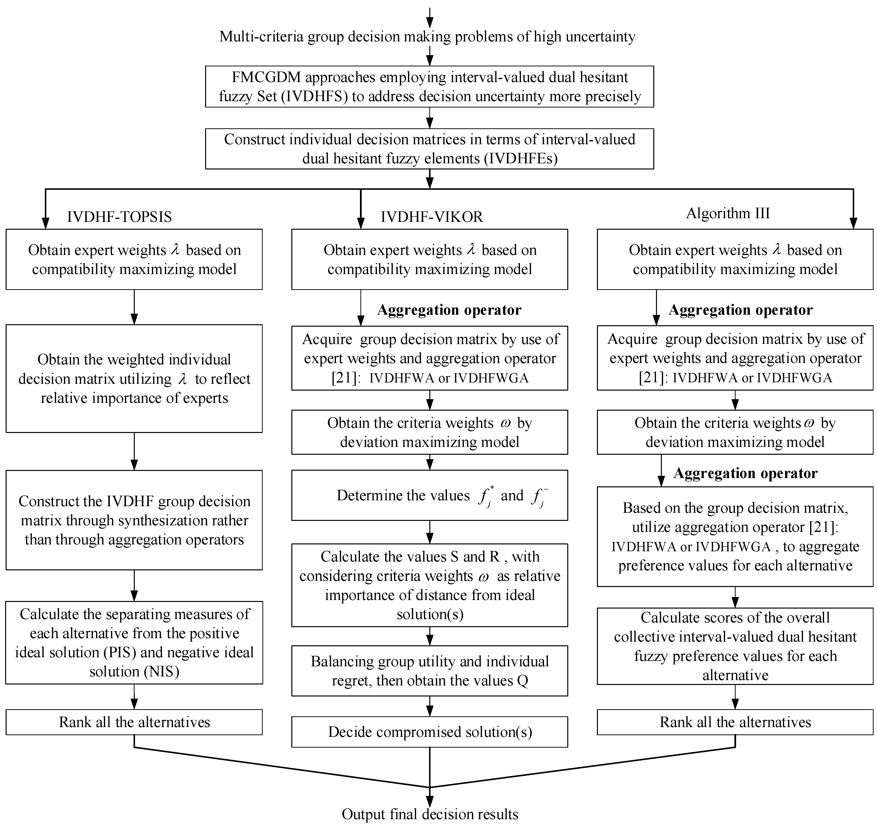
The above-proposed IVDHF-TOPSIS and IVDHF-VIKOR extend conventional TOPSIS and VIKOR to effectively tackle complex MCGDM with decision hesitancy and without weighting information (i.e., expert weights and attribute weights are totally unknown). Also they still can retain simple and straightforward decision making procedures, as shown in Figure 3 for clarity.

To further analytically compare with widely-used aggregation-operators-based approaches [11,29], we here extend the MCDM approach with IVDHF preferences by Ju, et al. [27] to group setting and propose the following Algorithm III, which employs the IVDHFWA operator in Definition 2.7 for information aggregation. Decision making procedures of Algorithm III are also shown in Figure 3. It is worth noticing that, the aggregation-operators-based approach normally at least needs aggregation operators at two stages: (i) aggregate individual decision matrices into collective (group) decision matrix; (ii) aggregate collective (group) decision matrix to derive the final scores of all alternatives.

Algorithm III. Aggregation-operators-based approach for FMCGDM under IVDHF environments.

Step III-1. Determine the weighting vector $\lambda$ for decision makers by model (M-1).

Step III-2. Aggregate each individual IVDHF decision matrix ${\tilde{R}}^k={({\tilde{r}}_{ij}^k)}_{n\times m}(k=1,2,...,t)$ into the IVDHF group decision matrix $\tilde{R}={({\tilde{r}}_{ij})}_{n\times m}$ by the IVDHFWA operator [27], where

$${\tilde{r}}_{ij}=({\tilde{h}}_{ij},{\tilde{g}}_{ij})={\cup }_{[{\mu }_{ij}^{Lk},{\mu }_{ij}^{Uk}]\in {\tilde{h}}_{ij}^k,[{\nu }_{ij}^{Lk},{\nu }_{ij}^{Uk}]\in {\tilde{g}}_{ij}^k}\{\left\{\left[1-{\displaystyle \prod _{k=1}^t{(1-{\mu }_{ij}^{Lk})}^{{\lambda }_k}},1-{\displaystyle \prod _{k=1}^t{(1-{\mu }_{ij}^{Uk})}^{{\lambda }_k}}\right]\right\},\left\{\left[{\displaystyle \prod _{k=1}^t{({\nu }_{ij}^{Lk})}^{{\lambda }_k}},{\displaystyle \prod _{k=1}^t{({\nu }_{ij}^{Uk})}^{{\lambda }_k}}\right]\right\}\}.$$

(33)

Step III-3. Obtain weighting vector $\omega$ for criteria based on the above group decision matrix $\tilde{R}={({\tilde{r}}_{ij})}_{n\times m}$ by model (M-2).

Step III-4. Use the IVDHFWA operator [27] to obtain the overall collective values ${\tilde{r}}_i$ in terms of IVDHFEs for each alternative $x_i(i=1,2,...,n)$, where

$${\tilde{r}}_i=({\tilde{h}}_i,{\tilde{g}}_i)={\cup }_{[{\mu }_{ij}^L,{\mu }_{ij}^U]\in {\tilde{h}}_{ij},[{\nu }_{ij}^L,{\nu }_{ij}^U]\in {\tilde{g}}_{ij}}\{\left\{\left[1-{\displaystyle \prod _{j=1}^m{(1-{\mu }_{ij}^L)}^{{\omega }_j}},1-{\displaystyle \prod _{j=1}^m{(1-{\mu }_{ij}^U)}^{{\omega }_j}}\right]\right\},\left\{\left[{\displaystyle \prod _{j=1}^m{({\nu }_{ij}^L)}^{{\omega }_j}},{\displaystyle \prod _{j=1}^m{({\nu }_{ij}^U)}^{{\omega }_j}}\right]\right\}\}.$$

(34)

Step III-5. Calculate scores $S({\tilde{r}}_i)$ for each alternative $x_i$ by Equation (4).

Step III-6. Ranking all the alternatives according to the descending orders of $S({\tilde{r}}_i)$.

Subsequently, based on the comparative illustration in Figure 3, advantages that the proposed approaches IVDHF-TOPSIS and IVDHF-VIKOR attain are analyzed as follows.

(i) IVDHF-TOPSIS and IVDHF-VIKOR hold adaptability and flexibility in tackling MCGDM with decision hesitancy. The employed expression tool of IVDHFS can depict decision maker’s hesitant preferences with not only membership degrees but also non-membership degrees, and especially can accommodate the highly-uncertain decision situations where decision makers are only capable of indicating their hesitancy with interval-values rather than crisp ones.

(ii) IVDHF-TOPSIS and IVDHF-VIKOR can avoid information loss to different extents in comparison with the aggregation-operators-based approaches like Algorithm III. As can be seen from Figure 3, IVDHF-TOPSIS avoids using any aggregation operator by introducing the synthesized IVDHF group decision matrix; IVDHF-VIKOR only needs information aggregation at the first stage, while Algorithm III heavily depends on aggregation operations at two stages to yield final ranking orders. Generally, decision making procedures in IVDHF-TOPSIS and IVDHF-VIKOR are both based on the differentiating ideas by measuring distances from ideal solutions rather than through aggregation operators (i.e., Step III-2 and Step III-4) used in Algorithm III, thus can help IVDHF-TOPSIS and IVDHF-VIKOR alleviate information loss that would be caused by use of aggregation operation.

(iii) IVDHF-TOPSIS and IVDHF-VIKOR also can alleviate computation complexity for multi-criteria decision making based on dual hesitant fuzzy information. IVDHFS enables decision maker’s to express their hesitant preferences more effectively and comprehensively, but on the other hand, processing the compound expression structure (i.e., $\langle x,\tilde{h}(x),\tilde{g}(x)\rangle$) increases computational complexity in information aggregation, such as can be seen from the Equations (33) and (34) used in Algorithm III. While, IVDHF-TOPSIS obtains separating values (i.e., as shown in Equations (21) and (22)) only by utilizing distance measures to compute relative closeness to the positive ideal solution, IVDHF-VIKOR is also capable of differentiating alternatives by utilizing distance measures (i.e., as shown in Equation (28)) to simultaneously consider maximum group utility and minimum individual regret. Additionally, IVDHFS can reduce to DHFS when we set upper bounds and lower bounds as equal in $\tilde{h}(x)$ and $\tilde{g}(x)$, thus the proposed IVDHF-TOPSIS and IVDHF-VIKOR, in comparison with aggregation-operators-based approaches, still are capable of alleviating computation complexity under dual hesitant fuzzy environments.

In what follows, numerical examples are presented to verify our proposed approaches.

5. Numerical Examples

5.1. Case Study

In order to mitigate the damage of natural or man-made disaster in highly populated areas, more and more municipal governments in China have established emergency department to provide rescue capacity. Consider one of the emergency management problems (adapted from Ju, et al. [14]), as explained in Section 2.1, the community development department (CDD) of a major city that holds a state-level special economic zone needs to regularly evaluate a set of alternative response solutions against urban fire hazards.

Suppose there are three alternative rescue plans $\left\{x_1,x_2,x_3\right\}$ for evaluation against an urban fire hazard. Three expert teams $d_k(k=1,2,3)$, i.e., employees team ($d_1$), external experts team ($d_2$), and senior management team ($d_3$), have been organized to evaluate the alternatives under four criteria: ($c_1$) accident identifying capacity, ($c_2$) rescuing capacity, ($c_3$) emergency response resources supplying capacity, and ($c_4$) after-accident management capacity. Due to the highly-unstructured characteristics of this management activity, assessment values are hardly to be assigned with crisp numbers and decision makers are often inclined to be hesitant or irresolute in assigning those assessments. Therefore, in this case study, decision makers are empowered to provide their preferences in terms of IVDHFEs on the response solutions $x_i(i=1,2,3)$ under the four criteria $c_j(j=1,2,3,4)$. Then, three IVDHF matrices ${\tilde{R}}^k={({\tilde{r}}_{ij}^k)}_{3\times 4}={({\tilde{h}}_{ij}^k,{\tilde{g}}_{ij}^k)}_{3\times 4},(k=1,2,3)$ are collected and listed in following

Table 2. The IVDHF decision matrix ${\tilde{R}}^1={({\tilde{h}}_{ij}^1,{\tilde{g}}_{ij}^1)}_{3\times 4}$ provided by d₁.

${\tilde{R}}^1$	$c_1$	$c_2$	$c_3$	$c_4$
$x_1$	({[0.3, 0.5]},{[0.1, 0.2]})	({[0.1, 0.4]},{[0.2, 0.3],[0.3, 0.4]})	({[0.2, 0.4]},{[0.4, 0.5]})	({[0.6, 0.7],[0.7, 0.8]},{[0.1, 0.2]})
$x_2$	({[0.4, 0.7]},{[0.2, 0.3]})	({[0.5, 0.6]},{[0.1, 0.2]})	({[0.2, 0.3]},{[0.5, 0.6][0.6, 0.7]})	({[0.4, 0.5]},{[0.2, 0.4]})
$x_3$	({[0.6, 0.8]},{[0.1, 0.2]})	({[0.3, 0.4],[0.4, 0.5]},{[0.4, 0.5]})	({[0.5, 0.6],[0.7, 0.8]},{[0.1, 0.2]})	({[0.5, 0.7]},{[0.1, 0.2],[0.2, 0.3]})

,

Table 3. The IVDHF decision matrix ${\tilde{R}}^2={({\tilde{h}}_{ij}^2,{\tilde{g}}_{ij}^2)}_{3\times 4}$ provided by d₂.

${\tilde{R}}^2$	$c_1$	$c_2$	$c_3$	$c_4$
$x_1$	({[0.1, 0.2],[0.2, 0.3]},{[0.3, 0.4]})	({[0.6, 0.7]},{[0.1, 0.2],[0.2, 0.3]})	({[0.3, 0.4],[0.4, 0.5]},{[0.4, 0.5]})	({[0.4, 0.7]},{[0.2, 0.3]})
$x_2$	({[0.7, 0.8]},{[0.1, 0.2]})	({[0.2, 0.3]},{[0.5, 0.6]})	({[0.6, 0.8]},{[0.1, 0.2]})	({[0.3, 0.5]},{[0.3, 0.4]})
$x_3$	({[0.4, 0.5]},{[0.3, 0.4],[0.4, 0.5]})	({[0.7, 0.8]},{[0.1, 0.2]})	({[0.2, 0.5]},{[0.3, 0.4]})	({[0.3, 0.4]},{[0.2, 0.4],[0.4, 0.5]})

and

Table 4. The IVDHF decision matrix ${\tilde{R}}^3={({\tilde{h}}_{ij}^3,{\tilde{g}}_{ij}^3)}_{3\times 4}$ provided by d₃.

${\tilde{R}}^3$	$c_1$	$c_2$	$c_3$	$c_4$
$x_1$	({[0.2, 0.4]},{[0.3, 0.4],[0.5, 0.6]})	({[0.6, 0.7]},{[0.1, 0.2],[0.2, 0.3]})	({[0.1, 0.2] },{[0.5, 0.6],[0.6, 0.7]})	({[0.3, 0.5]},{[0.1, 0.3],[0.3, 0.5]})
$x_2$	({[0.4, 0.6],[0.6, 0.7]},{[0.1, 0.3]})	({[0.3, 0.5]},{[0.1, 0.3],[0.4, 0.5]})	({[0.4, 0.6]},{[0.3, 0.4]})	({[0.7, 0.8]},{[0.1, 0.2]})
$x_3$	({[0.7, 0.8]},{[0.1, 0.2]})	({[0.5, 0.6]},{[0.3, 0.4]})	({[0.6, 0.7]},{[0.1, 0.2],[0.2, 0.3]})	({[0.6, 0.7]},{[0.1, 0.3]})

.

Now we can apply the proposed approaches IVDHF-TOPSIS and IVDHF-VIKOR to resolve this problem.

Firstly, according to the steps in Algorithm I, decision making procedures of IVDHF-TOPSIS are carried out in the following.

Step I-1. Determine the weighting vector for decision makers by model (M-1):

λ = (0.3305, 0.3237, 0.3458).

Step I-2. Transform the three individual IVDHF decision matrices ${\tilde{R}}^k={({\tilde{r}}_{ij}^k)}_{3\times 4}(k=1,2,3)$ (as in Table 2, Table 3 and Table 4) into the weighted individual decision matrices ${\overline{\tilde{R}}}^k={({\overline{\tilde{r}}}_{ij}^k)}_{3\times 4}$, shown as

Table 5. The weighted individual decision matrix ${\overline{\tilde{R}}}^1={({\overline{\tilde{h}}}_{ij}^1,{\overline{\tilde{g}}}_{ij}^1)}_{3\times 4}$.

${\overline{\tilde{R}}}^1$	$c_1$	$c_2$	$c_3$	$c_4$
$x_1$	({[0.11, 0.2047]},{[0.4672, 0.5875]})	({[0.0342, 0.1553]},{[0.5875, 0.6717],[0.6717, 0.7387]})	({[0.0711, 0.1553]},{[0.7387, 0.7953]})	({[0.2613, 0.3283],[0.3283, 0.4125]},{[0.4672, 0.5875]})
$x_2$	({[0.1553, 0.328]},{[0.5875, 0.6717]})	({[0.2047, 0.2613]},{[0.4672, 0.5875]})	({[0.0711, 0.1112]},{[0.7953, 0.8447],[0.8447, 0.8888]})	({[0.1553, 0.2047]},{[0.5875, 0.7387]})
$x_3$	({[0.2613, 0.4125]},{[0.4672, 0.5875]})	({[0.1112, 0.1553],[0.1553, 0.2047]},{[0.7387, 0.7953]})	({[0.2047, 0.2613],[0.3283, 0.4125]},{[0.4672, 0.5875]})	({[0.2047, 0.3283]},{[0.4672, 0.5875],[0.5875, 0.6717]})

,

Table 6. The weighted individual decision matrix ${\overline{\tilde{R}}}^2={({\overline{\tilde{h}}}_{ij}^2,{\overline{\tilde{g}}}_{ij}^2)}_{3\times 4}$.

${\overline{\tilde{R}}}^2$	$c_1$	$c_2$	$c_3$	$c_4$
$x_1$	({[0.0335, 0.0697],[0.0697, 0.109]},{[0.6772, 0.7433]})	({[0.2567, 0.3228]},{[0.4746, 0.5939],[0.5939, 0.6772]})	({[0.109, 0.1524],[0.1524, 0.201]},{[0.7433, 0.799]})	({[0.1524, 0.3228]},{[0.5939, 0.6772]})
$x_2$	({[0.3228, 0.4061]},{[0.4746, 0.5939]})	({[0.0697, 0.109]},{[0.799, 0.8476]})	({[0.2567, 0.4061]},{[0.4746, 0.5939]})	({[0.109, 0.201]},{[0.6772, 0.7433]})
$x_3$	({[0.1524, 0.201]},{[0.6772, 0.7433],[0.7433, 0.799]})	({[0.3228, 0.4061]},{[0.4746, 0.5939]})	({[0.0697, 0.201]},{[0.6772, 0.7433]})	({[0.109, 0.1524]},{[0.5939, 0.7433],[0.7433, 0.799]})

and

Table 7. The weighted individual decision matrix ${\overline{\tilde{R}}}^3={({\overline{\tilde{h}}}_{ij}^3,{\overline{\tilde{g}}}_{ij}^3)}_{3\times 4}$.

${\overline{\tilde{R}}}^3$	$c_1$	$c_2$	$c_3$	$c_4$
$x_1$	({[0.0743, 0.1619]},{[0.6595, 0.7284],[0.7869, 0.8381]})	({[0.2716, 0.3405]},{[0.451, 0.5732],[0.5732, 0.6595]})	({[0.0358, 0.0743]},{[0.7869, 0.8381],[0.8381, 0.884]})	({[0.116, 0.2131]},{[0.451, 0.6595],[0.6595, 0.7869]})
$x_2$	({[0.1619, 0.2716],[0.2716, 0.3405]},{[0.451, 0.6595]})	({[0.116, 0.2131]},{[0.451, 0.6595],[0.7284, 0.7869]})	({[0.1619, 0.2716]},{[0.6595, 0.7284]})	({[0.3405, 0.4268]},{[0.451, 0.5732]})
$x_3$	({[0.3405, 0.4268]},{[0.451, 0.5732]})	({[0.2131, 0.2716]},{[0.6595, 0.7284]})	({[0.2716, 0.3405]},{[0.451, 0.5732],[0.5732, 0.6595]})	({[0.2716, 0.3405]},{[0.451, 0.6595]})

.

Step I-3. By combining all the weighted individual decision matrices, we construct the synthesized IVDHF group decision matrix $\tilde{R}={({\tilde{r}}_{ij})}_{3\times 4}={({\tilde{h}}_{ij}^{},{\tilde{g}}_{ij}^{})}_{3\times 4}$, where the ${\tilde{h}}_{ij}^{}$ part of all elements are shown in

Table 8. ${\tilde{h}}_{ij}^{}$ part in the synthesized IVDHF group decision matrix $\tilde{R}=({\tilde{h}}_{ij}^{},{\tilde{g}}_{ij}^{})$.

${\tilde{h}}_{ij}^{}$	$c_1$	$c_2$	$c_3$	$c_4$
$x_1$	{[0.0335, 0.0697],[0.0697, 0.109],[0.0743, 0.1619],[0.1112, 0.2047]}	{[0.0342, 0.1553],[0.2567, 0.3228],[0.2716, 0.3405]}	{[0.0358, 0.0743],[0.0711, 0.1553],[0.109, 0.1524],[0.1524, 0.201]}	{[0.116, 0.2131],[0.1524, 0.3228],[0.2613, 0.3283],[0.3283, 0.4125]}
$x_2$	{[0.1619, 0.2716],[0.1553, 0.328],[0.2716, 0.3405],[0.3228, 0.4061]}	{[0.0697, 0.109],[0.116, 0.2131],[0.2047, 0.2613]}	{[0.0711, 0.1112],[0.1619, 0.2716],[0.2567, 0.4061]}	{[0.109, 0.201],[0.1553, 0.2047],[0.3405, 0.4268]}
$x_3$	{[0.1524, 0.201],[0.2613, 0.4125],[0.3405, 0.4268]}	{[0.1112, 0.1553],[0.1553, 0.2047],[0.2131, 0.2716],[0.3228, 0.4061]}	{[0.0697, 0.201],[0.2047, 0.2613],[0.2716, 0.3405],[0.3283, 0.4125]}	{[0.109, 0.1524],[0.2047, 0.3283],[0.2716, 0.3405]}

and the ${\tilde{g}}_{ij}^{}$ part of all elements are shown in

Table 9. ${\tilde{g}}_{ij}^{}$ part of synthesized IVDHF group decision matrix $\tilde{R}=({\tilde{h}}_{ij}^{},{\tilde{g}}_{ij}^{})$.

${\tilde{g}}_{ij}^{}$	$c_1$	$c_2$	$c_3$	$c_4$
$x_1$	{[0.4672, 0.5875],[0.6595, 0.7284],[0.6772, 0.7433],[0.7869, 0.8381]}	{[0.451, 0.5732],[0.4746, 0.5939],[0.5732, 0.6595],[0.5875, 0.6717],[0.5939, 0.6772],[0.6717, 0.7387]}	{[0.7387, 0.7953],[0.7433, 0.799],[0.7869, 0.8381],[0.8381, 0.884]}	{[0.4672, 0.5875],[0.451, 0.6595],[0.5939, 0.6772],[0.6595, 0.7869]}
$x_2$	{[0.4746, 0.5939],[0.451, 0.6595],[0.5875, 0.6717]}	{[0.4672, 0.5875],[0.451, 0.6595],[0.7284, 0.7869],[0.799, 0.8476]}	{[0.4746, 0.5939],[0.6595, 0.7284],[0.7953, 0.8447],[0.8447, 0.8888]}	{[0.451, 0.5732],[0.5875, 0.7387],[0.6772, 0.7433]}
$x_3$	{[0.451, 0.5732],[0.4672, 0.5875],[0.6772, 0.7433],[0.7433, 0.799]}	{[0.4746, 0.5939],[0.6595, 0.7284],[0.7387, 0.7953]}	{[0.451, 0.5732],[0.4672, 0.5875],[0.5732, 0.6595],[0.6772, 0.7433]}	{[0.4672, 0.5875],[0.451, 0.6595],[0.5875, 0.6717],[0.5939, 0.7433],[0.7433, 0.799]}

.

Step I-4. Determine the positive ideal solution (PIS) $X^{+}$ and negative ideal solutions (NIS) $X^{-}$, and then calculate the separating measures from the PIS and NIS for each alternative:

$$d_1^{+}=4.2815,d_1^{-}=1.5613;d_2^{+}=4.0922,d_2^{-}=1.7824;d_3^{+}=3.9409,d_3^{-}=\mathrm{1.8947.}$$

Step I-5. Calculate the relative closeness to the ideal solution $c_i$:

c₁ = 0.2672, c₂ = 0.3034,, c₃ = 0.3247.

Step I-6. Rank the alternatives according to the descending order of $c_i$:

$$x_3\succ x_2\succ x_1.$$

Thus, IVDHF-TOPSIS identifies the solution $x_3$ as the most appropriate alternative for this case.

Next, we apply the proposed IVDHF-VIKOR in Algorithm II to prioritize solutions in the above case. Decision making procedures of IVDHF-VIKOR are constructed as follows.

Step II-1. Same as Step I-1, we have obtained the weighting vector for decision makers:

λ = (0.3305, 0.3237, 0.3458).

Step II-2. Utilize the IVDHFWA operator in Definition 2.7 to aggregate individual decision matrices ${\tilde{R}}^k={({\tilde{r}}_{ij}^k)}_{3\times 4}(k=1,2,3)$ into IVDHF group decision matrix ${\tilde{R}}_{IVDHFWA}={({\tilde{r}}_{ij})}_{3\times 4}={({\tilde{h}}_{ij}^{},{\tilde{g}}_{ij}^{})}_{3\times 4}$, where the ${\tilde{h}}_{ij}^{}$ part of all elements are shown in

Table 10. ${\tilde{h}}_{ij}^{}$ part of IVDHF Group decision matrix ${\tilde{R}}_{IVDHFWA}=({\tilde{h}}_{ij}^{},{\tilde{g}}_{ij}^{})$.

${\tilde{h}}_{ij}^{}$	$c_1$	$c_2$	$c_3$	$c_4$
$x_1$	{[0.2048, 0.38],[0.2345, 0.4062]}	{[0.4771, 0.6228]}	{[0.202, 0.3372],[0.2408, 0.3752]}	{[0.4465, 0.642],[0.4967, 0.6869]}
$x_2$	{[0.5206, 0.7094],[0.5833, 0.7369]}	{[0.346, 0.4821]}	{[0.4213, 0.6155]}	{[0.5037, 0.6358]}
$x_3$	{[0.5871, 0.7309]}	{[0.5264, 0.6346],[0.5499, 0.6559]}	{[0.4611, 0.6108],[0.5448, 0.6904]}	{[0.4839, 0.6245]}

and the ${\tilde{g}}_{ij}^{}$ part of all elements are shown in

Table 11. ${\tilde{g}}_{ij}^{}$ part of IVDHF Group decision matrix ${\tilde{R}}_{IVDHFWA}=({\tilde{h}}_{ij}^{},{\tilde{g}}_{ij}^{})$.

${\tilde{g}}_{ij}^{}$	$c_1$	$c_2$	$c_3$	$c_4$
$x_1$	{[0.2087, 0.3181],[0.249, 0.366]}	{[0.1257, 0.2287],[0.1598, 0.2631],[0.1574, 0.2608],[0.2, 0.3],[0.1438, 0.2515],[0.1827, 0.2893],[0.1799, 0.2868],[0.2287, 0.3299]}	{[0.4321, 0.5325],[0.4602, 0.5617]}	{[0.1252, 0.2624],[0.183, 0.3131]}
$x_2$	{[0.1257, 0.2631]}	{[0.1684, 0.3284],[0.2719, 0.3918]}	{[0.2489, 0.3654],[0.2643, 0.3845]})	{[0.1794, 0.3147]}
$x_3$	{[0.1427, 0.2503],[0.1566, 0.2691]}	{[0.2312, 0.3441]}	{[0.1427, 0.2503],[0.1814, 0.288]}	{[0.1252, 0.288],[0.1566, 0.3096],[0.1574, 0.3293],[0.197, 0.3539]}

.

Step II-3. Obtain the weighting vector for criteria according to model (M-2):

ω = (0.3493, 0.1956, 0.3849, 0.0703)^T.

Step II-4. Determine the best values $f_j^{*}$ and the worst values $f_j^{-}$:

$$f_1^{*}=\left(\left\{\left[0.5871,0.7309\right]\right\},\{\left[0.1427,0.2503\right],\left[0.1566,0.2691\right]\}\right),$$

$$\begin{array}{l}{f}_1^{-}=\left(\left\{\left[0.2048,0.38\right],\left[0.2345,0.4062\right]\right\},\{\left[0.2087,0.3181\right],\left[0.249,0.366\right]\}\right),\\ f_2^{*}=(\left\{\left[0.4771,0.6228\right]\right\},\{\left[0.1257,0.2287\right],\left[0.1598,0.2631\right],\left[0.1574,0.2608\right],\left[0.2,0.3\right],\left[0.1438,0.2515\right],\left[0.1827,0.2893\right],\left[0.1799,0.2868\right],\left[0.2287,0.3299\right]\})\\ f_2^{-}=\left(\left\{\left[0.346,0.4821\right]\right\},\{\left[0.1684,0.3284\right],\left[0.2719,0.3918\right]\}\right),\\ f_3^{*}=\left(\left\{\left[0.4611,0.6108\right],\left[0.5448,0.6904\right]\right\},\{\left[0.1427,0.2503\right],\left[0.1814,0.288\right]\}\right),\\ f_3^{-}=\left(\left\{\left[0.202,0.3372\right],\left[0.2408,0.3752\right]\right\},\{\left[0.4321,0.5325\right],\left[0.4602,0.5617\right]\}\right),\\ f_4^{*}=\left(\left\{\left[0.4465,0.642\right],\left[0.4967,0.6869\right]\right\},\{\left[0.1252,0.2624\right],\left[0.183,0.3131\right]\}\right)\\ f_4^{-}=\left(\left\{\left[0.4839,0.6245\right]\right\},\{\left[0.1252,0.288\right],\left[0.1566,0.3096\right],\left[0.1574,0.3293\right],\left[0.197,0.3539\right]\}\right).\end{array}$$

Step II-5. Calculate the normalized fuzzy distance $d_{ij}$:

d₁₁ = 1, d₂₁ = 0.11, d₃₁ = 0, d₁₂ = 0, d₂₂ = 1, d₃₂ = 0.5415, d₁₃ = 1, d₂₃ = 0.3119, d₃₃ = 0, d₁₄ = 0, d₂₄ = 0.8544, d₃₄ = 1.

Step II-6. Compute $S_i$ and $R_i$:

S₁ = 0.7342, S₂ = 0.4141, S₃ = 0.1762, R₁ = 0.3849, R₂ = 0.1956, R₃ = 0.1059.

Step II-7. Suppose $v$ = 0.5, then we can obtain $Q_i(i=1,2,3)$ as

Q₁ = 1, Q₂ = 0.3739, Q₃ = 0.

Step II-8. Rank the alternatives according to the ascending order of $S$, $R$ and $Q$, respectively. Then we get three ranked lists as shown in

Table 12. Ranked results and the compromise solutions for all alternatives.

	Rescue Plans			Ranking Orders	Compromise Solution
	$x_1$	$x_2$	$x_3$
$S$	0.7342	0.4141	0.1762	$x_3\succ x_2\succ x_1$	$x_3$
$R$	0.3849	0.1956	0.1059	$x_3\succ x_2\succ x_1$	$x_3$
$Q(v=0.5)$	1	0.3739	0	$x_3\succ x_2\succ x_1$	$x_3$

.

Step II-9. Because solution $x_3$ satisfies the conditions C1 and C2 simultaneously, $x_3$ is thus the unique compromise solution.

Therefore, IVDHF-TOPSIS and IVDHF-VIKOR output the same ranking results for all three rescue plans; both identify response solution $x_3$ as the most appropriate one.

5.2. Comparison with Aggregation-Operators-Based Approach

In order to further verify the effectiveness of the proposed approaches IVDHF-TOPSIS and IVDHF-VIKOR, we here apply the aggregation-operators-based approach Algorithm III to resolve the same case in Section 5.1 then compare the ranking results obtained by all the three approaches. After calculation, Algorithm III output the final ranking result as $x_3\succ x_2\succ x_1$. For clarity, ranking results yielded by all the three algorithms are compared in

Table 13. Ranking results obtained by Algorithms I–III.

Methods	Ranking Results
Algorithm I: IVDHF-TOPSIS	$x_3\succ x_2\succ x_1$
Algorithm II: IVDHF-VIKOR	$x_3\succ x_2\succ x_1$
Algorithm III: Aggregation-operators-based approach	$x_3\succ x_2\succ x_1$

.

As can be seen from Table 13, all the three approaches identify the same ranking order for the three response solutions, which verifies all the three types of FMCGDM approaches are effective in differentiating decision solutions. According to analysis in Section 4.3, IVDHF-TOPSIS and IVDHF-VIKOR avoid using multiple aggregation operators so that they are capable of alleviating potential information loss and reducing computational complexity FMCGDM under hesitant fuzzy environments. Therefore, the proposed IVDHF-TOPSIS and IVDHF-VIKOR are effective and indispensable approaches in supporting multi-criteria decision making characterized with decision hesitancy.

6. Conclusions

Increasing instances of natural and manmade disasters have caused great losses to local society and economics, which also have forced governments to bring emergency management to the center of the vital task of planning and implementing sustainable community development. Sustainable community planning must include emergency response solutions to identifiable risks of potential disasters. Suitable approaches for evaluating alternative response solutions also must be developed to support community development departments maintaining their emergency response solution repository.

Emergency response solutions evaluation (ERSE) generally can be categorized as a type of complex multi-criteria group decision making problem under uncertain environments, in which decision makers are often hesitant or irresolute when assessing fuzzy objects. Due to the lack of fuzzy multi-criteria group decision making (FMCGDM) approaches for ERSE with presence of decision hesitancy, in this paper, we proposed two effective FMCGDM approaches: IVDHF-TOPSIS and IVDHF-VIKOR. We employed IVDHFS to elicit decision hesitancy caused by uncertainties more effectively and comprehensively. Based on decision matrices provided in terms of IVDHFEs by decision makers, we developed the deviation maximizing model and the compatibility maximizing model to objectively determine unknown criteria weights and expert weights, respectively. In comparison with widely used aggregation-operators-based approach, IVDHF-TOPSIS and IVDHF-VIKOR are capable of alleviating information loss by avoiding multiple use of aggregation operators and reducing computational complexity in processing hesitant fuzzy preferences. Numerical examples have verified the effectiveness of both IVDHF-TOPSIS and IVDHF-VIKOR.

Limitations of this paper exist and also point out our future research directions: further real-world case researches should be carried out to refine the proposed approaches; when confronted with ERSE problems in more complicate emergency scenarios, such as correlations among criteria and order inducing attitudes, extending the proposed methods to accommodate these problems would be another future research direction; to facilitate Internet-based application, a distributed decision support system should be implemented.

As the proposed methods are not only easy to understand and ready to implement, but also generalizable, they would be important and valuable tools for prioritizing alternatives and assessing performances in many other operational management areas in practice.

References

1. Schaffer, R.; Deller, S.C.; Marcouiller, D.W. Community Economics: Linking Theory and Practice; Wiley-Blackwell: New York, NY, USA, 2004. [Google Scholar]
2. Schneider, R.O. Emergency Management and Sustainability: Defining a Profession; Charles C Thomas Pub Ltd.: Springfield, Illinois, 2013. [Google Scholar]
3. Jenvald, J.; Morin, M.; Timpka, T.; Eriksson, H. Simulation as decision support in pandemic influenza preparedness and response. In Proceedings of the 4th ISCRAM Conference, Delft, The Netherlands, 13–16 May 2007; pp. 295–304.
4. Engelmann, H.; Fiedrich, F. Decision support for the members of an emergency operation centre after an earthquake. In Proceedings of the 4th ISCRAM Conference, Delft, The Netherlands, 13–16 May 2007; pp. 317–326.
5. Reniers, G.L.L.; Ale, B.J.M.; Dullaert, W.; Foubert, B. Decision support systems for major accident prevention in the chemical process industry: A developers’ survey. J. Loss Prev. Process Ind. 2006, 19, 604–620. [Google Scholar] [CrossRef]
6. Fogli, D.; Guida, G. Knowledge-centered design of decision support systems for emergency management. Decis. Support Syst. 2013, 55, 336–347. [Google Scholar] [CrossRef]
7. Ju, Y.B.; Wang, A.H.; You, T.H. Emergency alternative evaluation and selection based on ANP, DEMATEL, and TL-TOPSIS. Nat. Hazards. 2015, 75, S347–S379. [Google Scholar] [CrossRef]
8. Ju, Y.B.; Wang, A.H. Emergency alternative evaluation under group decision makers: A method of incorporating DS/AHP with extended TOPSIS. Expert Syst. Appl. 2012, 39, 1315–1323. [Google Scholar] [CrossRef]
9. Ju, Y.B.; Wang, A.H. Extension of VIKOR method for multi-criteria group decision making problem with linguistic information. Appl. Math. Model. 2013, 37, 3112–3125. [Google Scholar] [CrossRef]
10. Kahraman, C.; Onar, S.C.; Oztaysi, B. Fuzzy Multicriteria Decision-Making: A Literature Review. Int. J. Comput. Int. Syst. 2015, 8, 637–666. [Google Scholar] [CrossRef]
11. Qi, X.; Liang, C.; Zhang, J. Generalized cross-entropy based group decision making with unknown expert and attribute weights under interval-valued intuitionistic fuzzy environment. Comput. Ind. Eng. 2015, 79, 52–64. [Google Scholar] [CrossRef]
12. Mardani, A.; Jusoh, A.; Zavadskas, E.K. Fuzzy multiple criteria decision-making techniques and applications—Two decades review from 1994 to 2014. Expert Syst. Appl. 2015, 42, 4126–4148. [Google Scholar] [CrossRef]
13. Liu, Y.; Fan, Z.P.; Zhang, Y. Risk decision analysis in emergency response: A method based on cumulative prospect theory. Comput. Oper. Res. 2014, 42, 75–82. [Google Scholar] [CrossRef]
14. Ju, Y.B.; Wang, A.H.; Liu, X.Y. Evaluating emergency response capacity by fuzzy AHP and 2-tuple fuzzy linguistic approach. Expert Syst. Appl. 2012, 39, 6972–6981. [Google Scholar] [CrossRef]
15. Torra, V.; Narukawa, Y. On hesitant fuzzy sets and decision. In The 18th IEEE International Conference on Fuzzy Systems, Jeju Island, Korea, 20–24 August 2009; pp. 1378–1382.
16. Torra, V. Hesitant fuzzy sets. Int. J. Intell. Syst. 2010, 25, 529–539. [Google Scholar] [CrossRef]
17. Montazer, G.A.; Saremi, H.Q.; Ramezani, M. Design a new mixed expert decision aiding system using fuzzy ELECTRE III method for vendor selection. Expert Syst. Appl. 2009, 36, 10837–10847. [Google Scholar] [CrossRef]
18. Chen, T.-Y. An interval type-2 fuzzy PROMETHEE method using a likelihood-based outranking comparison approach. Inf. Fusion. 2015, 25, 105–120. [Google Scholar] [CrossRef]
19. Park, J.H.; Park, I.Y.; Kwun, Y.C.; Tan, X.G. Extension of the TOPSIS method for decision making problems under interval-valued intuitionistic fuzzy environment. Appl. Math. Model. 2011, 35, 2544–2556. [Google Scholar] [CrossRef]
20. Zhang, X.L.; Xu, Z.S. The TODIM analysis approach based on novel measured functions under hesitant fuzzy environment. Knowl.-Based Syst. 2014, 61, 48–58. [Google Scholar] [CrossRef]
21. Zhang, X.L.; Xu, Z.S. Hesitant fuzzy QUALIFLEX approach with a signed distance-based comparison method for multiple criteria decision analysis. Expert Syst. Appl. 2015, 42, 873–884. [Google Scholar] [CrossRef]
22. Chen, N.; Xu, Z.S. Hesitant fuzzy ELECTRE II approach: A new way to handle multi-criteria decision making problems. Inf. Sci. 2015, 292, 175–197. [Google Scholar] [CrossRef]
23. Peng, J.-J.; Wang, J.-Q.; Wang, J.; Yang, L.-J.; Chen, X.-H. An extension of ELECTRE to multi-criteria decision-making problems with multi-hesitant fuzzy sets. Inf. Sci. 2015, 307, 113–126. [Google Scholar] [CrossRef]
24. Zhu, B.; Xu, Z.S.; Xia, M.M. Dual Hesitant Fuzzy Sets. J. Appl. Math. 2012, 2012, 1–13. [Google Scholar] [CrossRef]
25. Farhadinia, B. Correlation for Dual Hesitant Fuzzy Sets and Dual Interval-Valued Hesitant Fuzzy Sets. Int. J. Intell. Syst. 2014, 29, 184–205. [Google Scholar] [CrossRef]
26. Zhu, B.; Xu, Z.S. Some results for dual hesitant fuzzy sets. J. Intell. Fuzzy Syst. 2014, 26, 1657–1668. [Google Scholar]
27. Ju, Y.B.; Liu, X.Y.; Yang, S.H. Interval-valued dual hesitant fuzzy aggregation operators and their applications to multiple attribute decision making. J. Intell. Fuzzy Syst. 2014, 27, 1203–1218. [Google Scholar]
28. Zhang, W.K.; Li, X.; Ju, Y.B. Some Aggregation Operators Based on Einstein Operations under Interval-Valued Dual Hesitant Fuzzy Setting and Their Application. Math. Probl. Eng. 2014, 2014, 1–15. [Google Scholar] [CrossRef]
29. Zhang, Z.; Wang, C.; Tian, D.; Li, K. Induced generalized hesitant fuzzy operators and their application to multiple attribute group decision making. Comput. Ind. Eng. 2014, 67, 116–138. [Google Scholar] [CrossRef]
30. Yue, Z. An avoiding information loss approach to group decision making. Appl. Math. Model. 2013, 37, 112–126. [Google Scholar] [CrossRef]
31. Xu, Z.S.; Zhang, X.L. Hesitant fuzzy multi-attribute decision making based on TOPSIS with incomplete weight information. Knowl.-Based Syst. 2013, 52, 53–64. [Google Scholar] [CrossRef]
32. Yoon, K.; Hwang, C. Multiple Attribute Decision Making: Methods and Applications; Springer: Berlin, Germany, 1981. [Google Scholar]
33. Opricovic, S. Fuzzy VIKOR with an application to water resources planning. Expert. Syst. Appl. 2011, 38, 12983–12990. [Google Scholar] [CrossRef]
34. Opricovic, S.; Tzeng, G.H. Compromise solution by MCDM methods: A comparative analysis of VIKOR and TOPSIS. Eur. J. Oper. Res. 2004, 156, 445–455. [Google Scholar] [CrossRef]
35. Park, J.H.; Cho, H.J.; Kwun, Y.C. Extension of the VIKOR method for group decision making with interval-valued intuitionistic fuzzy information. Fuzzy Optim. Decis. Mak. 2011, 10, 233–253. [Google Scholar] [CrossRef]
36. Zhang, X.L.; Xu, Z.S. Soft computing based on maximizing consensus and fuzzy TOPSIS approach to interval-valued intuitionistic fuzzy group decision making. Appl. Soft Comput. 2015, 26, 42–56. [Google Scholar] [CrossRef]
37. Zhao, X.F. TOPSIS method for interval-valued intuitionistic fuzzy multiple attribute decision making and its application to teaching quality evaluation. J. Intell. Fuzzy Syst. 2014, 26, 3049–3055. [Google Scholar]
38. Feng, X.; Zuo, W.L.; Wang, J.H.; Feng, L.Z. TOPSIS method for hesitant fuzzy multiple attribute decision making. J. Intell. Fuzzy Syst. 2014, 26, 2263–2269. [Google Scholar]
39. Liu, H.C.; You, J.X.; Chen, Y.Z.; Fan, X.J. Site selection in municipal solid waste management with extended VIKOR method under fuzzy environment. Environ. Earth Sci. 2014, 72, 4179–4189. [Google Scholar] [CrossRef]
40. Chang, T.H. Fuzzy VIKOR method: A case study of the hospital service evaluation in Taiwan. Inf. Sci. 2014, 271, 196–212. [Google Scholar] [CrossRef]
41. Zhang, N.; Wei, G. Extension of VIKOR method for decision making problem based on hesitant fuzzy set. Appl. Math. Model. 2013, 37, 4938–4947. [Google Scholar] [CrossRef]
42. Beg, I.; Rashid, T. TOPSIS for Hesitant Fuzzy Linguistic Term Sets. Int. J. Intell. Syst. 2013, 28, 1162–1171. [Google Scholar] [CrossRef]
43. Tavakkoli-Moghaddam, R.; Gitinavard, H.; Mousavi, S.; Siadat, A. An Interval-Valued Hesitant Fuzzy TOPSIS Method to Determine the Criteria Weights. In Outlooks and Insights on Group Decision and Negotiation; Kamiński, B., Kersten, G.E., Szapiro, T., Eds.; Springer International Publishing: Berline, Germany, 2015; Volume 218, pp. 157–169. [Google Scholar]
44. Liao, H.C.; Xu, Z.S. A VIKOR-based method for hesitant fuzzy multi-criteria decision making. Fuzzy Optim. Decis. Mak. 2013, 12, 373–392. [Google Scholar] [CrossRef]
45. Liao, H.; Xu, Z.; Zeng, X.-J. Hesitant Fuzzy Linguistic VIKOR Method and Its Application in Qualitative Multiple Criteria Decision Making. IEEE Trans. Fuzzy Syst. 2015, 23, 1343–1355. [Google Scholar] [CrossRef]
46. Wei, G.; Zhang, N.A. A multiple criteria hesitant fuzzy decision making with Shapley value-based VIKOR method. J. Intell. Fuzzy Syst. 2014, 26, 1065–1075. [Google Scholar]
47. Kohler, A.R.; Som, C. Risk preventative innovation strategies for emerging technologies the cases of nano-textiles and smart textiles. Technovation 2014, 34, 420–430. [Google Scholar] [CrossRef]
48. Chen, A.; Chen, N.; Li, J.M. During-incident process assessment in emergency management: Concept and strategy. Saf. Sci. 2012, 50, 90–102. [Google Scholar] [CrossRef]
49. Wan, H.; Yang, Q.; Yu, M.-H.; Fei, Q. Grid-based platform for disaster response plan simulation over Internet. Simul. Model. Pract. Theory 2008, 16, 379–386. [Google Scholar]
50. EEA. Late lessons from early warnings: the precautionary principle; European Environment Agency: Copehagen, Denmark, 2001. [Google Scholar]
51. Phillips, B.D.; Neal, D.M.; Webb, G. Introduction to Emergency Management; CRC Press: Boca Raton, Florida, 2012. [Google Scholar]
52. Sutikno; Suliswanto, M.S.W. The Development of Manufacturing Industry Cluster as an Effort of Economic Improvement Expansion in East Java. Procedia Soc. Behav. Sci. 2015, 211, 992–998. [Google Scholar] [CrossRef]
53. He, Z.; Xu, S.; Shen, W.; Long, R.; Yang, H. Overview of the development of the Chinese Jiangsu coastal wind-power industry cluster. Renew. Sustain. Energy Rev. 2016, 57, 59–71. [Google Scholar] [CrossRef]
54. Deng, Y.F.; Zheng, S.Z. Capability assessment for urban emergency incident readiness. J. Saf. Sci. Technol. 2006, 2, 10–14. [Google Scholar]
55. Tian, Y.L.; Yang, Q. Study on the evaluation index system model of the emergency capability on emergency. J. Basic Sci. Eng. 2008, 16, 200–2008. [Google Scholar]
56. Zadeh, L.A. Fuzzy sets. Inf. Control. 1965, 8, 338–353. [Google Scholar] [CrossRef]
57. Turksen, I.B. Interval valued fuzzy sets based on normal forms. Fuzzy Set Syst. 1986, 20, 191–210. [Google Scholar] [CrossRef]
58. Atanassov, K.T. Intuitionistic fuzzy sets. Fuzzy Set Syst. 1986, 20, 87–96. [Google Scholar] [CrossRef]
59. Atanassov, K.T.; Gargov, G. Interval valued intuitionistic fuzzy sets. Fuzzy Set Syst. 1989, 31, 343–349. [Google Scholar] [CrossRef]
60. Liao, H.C.; Xu, Z.S.; Zeng, X.J.; Merigó, J.M. Qualitative decision making with correlation coefficients of hesitant fuzzy linguistic term sets. Knowl.-Based Syst. 2015, 76, 127–138. [Google Scholar] [CrossRef]
61. Wang, J.-Q.; Wu, J.-T.; Wang, J.; Zhang, H.-Y.; Chen, X.-H. Interval-valued hesitant fuzzy linguistic sets and their applications in multi-criteria decision-making problems. Inf. Sci. 2014, 288, 55–72. [Google Scholar] [CrossRef]
62. Xu, Z.S.; Xia, M.M. Distance and similarity measures for hesitant fuzzy sets. Inf. Sci. 2011, 181, 2128–2138. [Google Scholar] [CrossRef]
63. Ju, Y.B. A new method for multiple criteria group decision making with incomplete weight information under linguistic environment. Appl. Math. Model. 2014, 38, 5256–5268. [Google Scholar] [CrossRef]
64. Xiao, Z.; Chen, W.; Li, L. A method based on interval-valued fuzzy soft set for multi-attribute group decision-making problems under uncertain environment. Knowl. Inf. Syst. 2013, 34, 653–669. [Google Scholar] [CrossRef]
65. Xu, Z. A Deviation-Based Approach to Intuitionistic Fuzzy Multiple Attribute Group Decision Making. Group Decis. Negot. 2010, 19, 57–76. [Google Scholar] [CrossRef]
66. Zhang, G.; Dong, Y.; Xu, Y. Consistency and consensus measures for linguistic preference relations based on distribution assessments. Inf. Fusion. 2014, 17, 46–55. [Google Scholar] [CrossRef]
67. Xu, J.; Wu, Z. A maximizing consensus approach for alternative selection based on uncertain linguistic preference relations. Comput. Ind. Eng. 2013, 64, 999–1008. [Google Scholar] [CrossRef]
68. Wang, Y.M. Using the method of maximizing deviations to make decision for multi-indices. Syst. Eng. Electron. 1997, 8, 21–26. [Google Scholar]
69. Chen, C.-T.; Pai, P.-F.; Hung, W.-Z. An Integrated Methodology using Linguistic PROMETHEE and Maximum Deviation Method for Third-party Logistics Supplier Selection. Int. J. Comput. Int. Syst. 2010, 3, 438–451. [Google Scholar] [CrossRef]
70. Opricovic, S.; Tzeng, G.H. Extended VIKOR method in comparison with outranking methods. Eur. J. Oper. Res. 2007, 178, 514–529. [Google Scholar] [CrossRef]
Figure 1. The motivation of emergency response solutions evaluation (ERSE).
Sustainability 08 00291 g001
Figure 2. Relations between different fuzzy representation models.
Sustainability 08 00291 g002
Figure 3. Flowcharts of IVDHF-TOPSIS, IVDHF-VIKOR, and Algorithm III (aggregation-operators-based approach).
Sustainability 08 00291 g003