Green Economy Performance and Green Productivity Growth in China’s Cities: Measures and Policy Implication

Abstract

Resource depletion and environmental degradation have become serious challenges for China’s sustainable development. This paper constructs indicators to assess China’s green economy performance and green productivity growth, in which economic expansion, resource conservation and environmental protection need to be incorporated simultaneously. For this purpose, we combine non-radial directional distance function and meta-frontier Malmquist productivity to develop the indicators. The methodology also allows for the decomposition of driving forces of China’s green economy. Moreover, the dataset employed in this paper allows for the evaluation of 275 cities in China during the period 2003–2012. The main findings are as follows. First, most of China’s cities did not perform efficiently in terms of the green economy, with an average score of only 0.233. Second, the growth rate of green productivity is slower than real GDP, and the green productivity growth in China is only moderate. Third, innovation is the main driving force of China’s green productivity growth, but the central region lags behind when it comes to green innovation. Fourth, artificial local protectionism and transport limitations impede the progress of cities that perform ineffectively in the green economy. Based on our empirical findings, we provide policy implications and suggestions for enhancing China’s green economy performance and productivity growth.

1. Background and Motivation

With remarkable economic growth in the last four decades, China has become the second-largest economy in terms of gross domestic production (GDP). However, this comes at the cost of energy depletion and environmental degradation. With an ever-increasing demand for energy, China has become the world’s largest energy consumer since 2010. Several forms of pollutants such as dust and sulfur dioxide (SO₂) have increased dramatically, accounting for about 30% and 26% (respectively) of the world’s total emissions in 2012. The substantially increased emissions of dust and SO₂ are the main contributors of the horrible haze problem in China. Air pollutants are a strong indicator as anyone who visits China (especially the North and East) in winter would attest to this problem. Air pollution severely affects human health. Coupled with this are energy depletion and environmental degradation; these issues threaten China’s sustainable development.

It is therefore imperative for China to achieve a new path of development, considering economic growth, resource conservation as well as environmental protection [1]. In general, an increasing share of total factor productivity (TFP) in output growth is regarded as an indicator of transformation to sustainable growth [2,3,4]. Thus, measuring green productivity growth can help evaluate China’s chances and potential of achieving a green economy. The main objective of this paper is to provide an assessment of green economy performance and green productivity growth in China at the city level.

Improving energy and pollutant emissions performance is critical for reducing energy consumption and pollutant emissions; it is therefore the central issue of green productivity growth [5]. Accordingly, the Chinese government has set several targets for energy conservation and emission mitigation. To be specific, China announced its intention to reduce energy intensity by 16% in the 12th Year Plan period between 2011 and 2015; the total emissions of SO₂ are required to be decreased by 8%; and the mitigation target for dust emission has also been set for several provinces (such as Shanxi). It should be noted that cities are the executives of targets for energy conservation and emission mitigation, thus, an in-depth analysis of energy and pollutant emissions performance can help determine whether cities could achieve the green targets set by central or provincial governments through efficiency improvement.

With regards to the environment, this paper primarily focuses on air pollutants. In previous literature—for instance, Panayotou et al. [6] and Auffhammer & Carson [7]—much more attention was paid to carbon dioxide (CO₂). However, as one who has ever visited or lived in China knows, in recent years, the air pollution problem has become the central issue of environmental degradation. SO₂ is one of the main contributors of China’s severe air pollution.

The contributions of this paper lie in the following aspects.

●

First, green economy performance (GEP) and green productivity growth indicator (GPGI) are constructed by incorporating economic expansion, resource conservation, and environmental protection simultaneously, all of which are the essentials in China’s green economy.

●

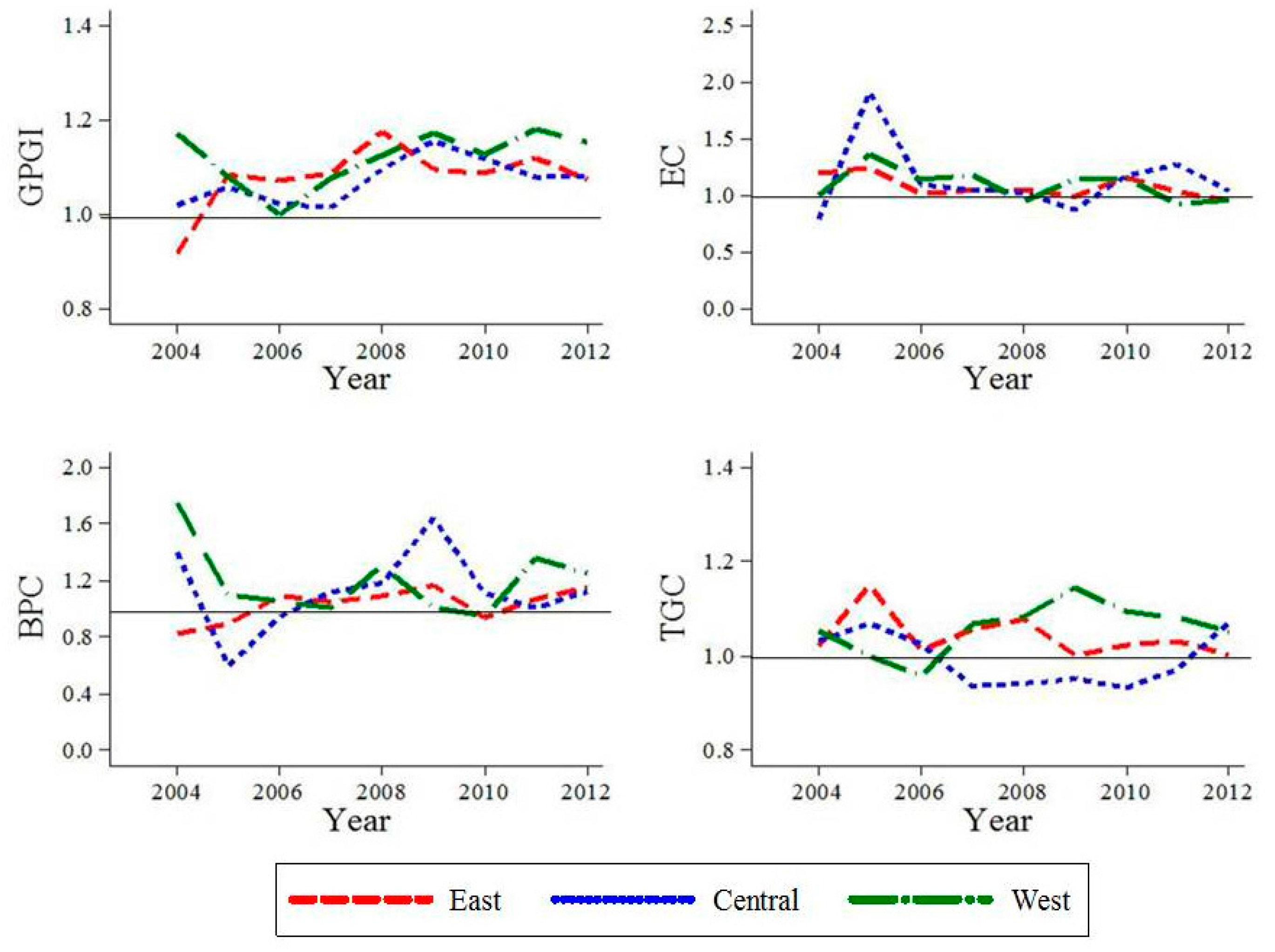
Second, the GPGI in each city is decomposed into three components, thus the driving forces in achieving green economy can be further analyzed, and the disparities across different regions could be compared in that the regional heterogeneities have been incorporated in the decomposition.

●

Third, the city panel data are compared to the empirical research, which could provide a much more detailed perspective than the widely used provincial dataset. To the best of our knowledge, few studies have employed a dataset on China’s cities in assessing energy and environmental performance as well as measuring green productivity growth. There are several studies employing China’s dataset at city level, for example, Au & Henderson [8,9], Ke [10]. However, studies using dataset at city level for empirically investigating China’s environmental economics are still rare. Dhakal [11] and Shi et al. [12] might be two exceptions, but only 35 largest cities are included in the former study and only 15 cities in the latter. In our paper, all cities except a few are included in the estimation.

The rest of this paper is organized as follows. Section 2 provides a literature review of related studies. Based on that, methodologies (NDDF, GEP, GPGI and their decomposition) are briefly introduced. Section 3 empirically analyzes the green economy performance and green productivity growth of China at the city level for the 2003–2012 period; the main driving forces of China’s green economy are also investigated. Section 4 concludes with several policy implications.

2. Methodology

The large and rapidly increasing energy consumption and pollution emissions have led green economy and sustainable development in China to become the subjects of intense discussion. In order to draw attention to the advantages of our model, we first provide a brief literature review before describing our methods in detail.

2.1. Literature Review

Green economy performance is defined as the efficiency of energy usage and pollutant emissions, while green productivity growth can be measured as the dynamic changes in energy and environmental performance [13,14,15]. Data envelop analysis (DEA) is a powerful tool for assessing energy and environmental performance. Numerous studies have applied the DEA method to investigate the efficiency of energy usage and pollution emissions (including CO₂). For example, Seiford & Zhu [16] evaluated the energy efficiency of 30 paper mills; Sözen et al. [17] assessed the operational and environmental performance of thermal power plants in Turkey; Wei et al. [18] estimated the CO₂ reduction potential of CO₂ for China’s provinces; Zhang et al. [19] computed the unified energy and carbon efficiency for 252 fossil fuel power plants in China; Honma & Hu [20] estimated total-factor energy efficiency scores for 47 regions across Japan; Yang et al. [21] assess green development efficiency of 31 provinces in China; Chen [22] builds a dynamic indicator to measure the ecological economic transition in China using slacks-based DEA model. Chen et al. [23] measure China’s industrial green development. Fei & Lin [24] assess agricultural energy efficiency in China’s agricultural sector. However, a substantial part of previous studies have employed the cross-sectional data to assess energy and environmental performance, rather than panel data which includes a time dimension. Thus, they cannot analyze the dynamic changes in efficiency performance, e.g., green productivity growth [25].

Zhou et al. [13] was the first to propose the Malmquist CO₂ emission performance index (MCPI); they investigated the changes in environmental efficiency by the DEA model. Essentially, the MCPI is based on the Shephard distance function for CO₂ emissions. It is therefore limited in measuring green productivity growth stemming from the fact that it cannot measure the dynamic performance change by increasing desirable outputs (GDP), while reducing undesirable outputs (pollutants) and energy inputs at the same time. However, it is key to simultaneously consider economic expansion, resource conservation, and pollutant mitigation when measuring green productivity growth.

Directional distance function (DDF) has drawn attention in that the method enables including economic expansion, resource conservation and pollutant mitigation in a single framework [26]. Chung et al. [27] first proposed the DDF method to examine environmental efficiency. Relevant studies on assessing environmental performance using the DDF method could be seen in Watanabe & Tanaka [28], Macpherson et al. [29], Halkos & Tzeremes [30], Ramli et al. [31] and Njuki & Ureta [32]. There are two limitations of the conventional DDF in the literature [33]. The first one is that it might overestimate efficiency when there are some slacks because the conventional DDF requires undesirable outputs (inputs) reduction and desirable output expansion at the same rate, which might lead to “slack-bias”. More discussions about the "slack-bias" could be seen in Zhang & Choi [33]. The second limitation is that a radial efficiency cannot provide a single-factor efficiency measure, such as pollutant emission efficiency [34].

Therefore, the non-radial DDF (NDDF) approach has been proposed by incorporating slacks and multiple scaling factors into the efficiency measurement. In order to measure the green productivity growth considering economic expansion, resource conservation, and pollutant mitigation simultaneously [35], this paper applies the method proposed by Oh & Lee [36] and Zhang et al. [37] by considering the non-radial slacks in the NDDF. The NDDF approach is appropriate by incorporating slacks and multiple scaling factors into the efficiency measurement, conducting the economic expansion, resource conservation and pollutant mitigation simultaneously, as well as overcoming the “slack bias” in DDF.

In addition, regional heterogeneities in production technology need to be incorporated because, in a country as large as China, there are substantial disparities across different regions, especially between more developed eastern China and less developed western China. Thus, the measurement results might be biased if we neglect the technological heterogeneities across regions [38]. Compared with Zhou et al. [13], the method applied in this paper methodologically combines the slack variables in NDDF and regional heterogeneities in the meta-frontier Malmquist index [37].

2.2. Methods

2.2.1. Green Production Technology

Suppose that there are $N$ assessed cities and each city is regarded as a decision-making unit (DMU). We assume that the DMUs use input vector $x\in {\Re }_{+}^m$ to jointly produce desirable output vector $y\in {\Re }_{+}^R$, meanwhile, undesirable outputs $b\in {\Re }_{+}^J$, are generated as byproducts of the production process. In this paper, the input vector contains capital ($K$), labor ($L$) and energy ($E$); the desirable output is GDP ($Y$), and SO₂ ($S$) and dust ($D$) as the undesirable byproducts of GDP. According to Färe et al. [39], the multi-output production technology can be described as:

$$P=\left\{\left(x,y,b\right):x \text{can produce} \left(y,b\right)\right\}$$

(1)

According to Färe & Grosskopf [40], the set $P$ is technically assumed to pose the standard axioms of the production theory: (1) inactivity is always possible; (2) finite amounts of inputs can only produce finite amounts of outputs; and (3) inputs and desirable outputs are often assumed to be strongly or freely disposable. For modeling the joint-production technology, the weak-disposability and null-jointness assumptions are also imposed on $P$ [39], indicating that:

(a) If $\left(x,y,b\right)\in P$ and $0\le \theta \le 1$, then $\left(x,\theta y,\theta b\right)\in P$. This property is termed as the weak-disposability condition, suggesting that pollution mitigation is not free, but can be reduced at the cost of desirable outputs.

(b) If $\left(x,y,b\right)\in P$ and $b=0$, then $y=0$. This condition is termed as null-jointness assumption. It implies that pollutants are unavoidable because desirable outputs cannot be produced without generating undesirable outputs.

In order to improve the comparability of observations in different years, this paper employs the global technology proposed by Oh [41] as the benchmark, using the whole sample to construct the technology frontier. More recently, Lin & Du [26] also used the idea of global technology. Based on Zhang & Choi [14], the technology $P$ for the $N$ cities in $T$ years showing constant returns to scale (CRS) can be formulated as follows:

$$P=\left\{\begin{array}{l}\left(K,L,E,Y,S,D\right):{\displaystyle \sum _{t=1}^T{\displaystyle \sum _{n=1}^N{\lambda }_{n,t}{K}_{n,t}}}\le K,{\displaystyle \sum _{t=1}^T{\displaystyle \sum _{n=1}^N{\lambda }_{n,t}{L}_{n,t}}}\le L,\\ {\displaystyle \sum _{t=1}^T{\displaystyle \sum _{n=1}^N{\lambda }_{n,t}{E}_{n,t}}}\le E,{\displaystyle \sum _{t=1}^T{\displaystyle \sum _{n=1}^N{\lambda }_{n,t}{Y}_{n,t}}}\ge Y,{\displaystyle \sum _{t=1}^T{\displaystyle \sum _{n=1}^N{\lambda }_{n,t}{S}_{n,t}}}=S,\\ {\displaystyle \sum _{t=1}^T{\displaystyle \sum _{n=1}^N{\lambda }_{n,t}{D}_{n,t}}}=D,{\lambda }_{n,t}\ge 0,n=1,\dots ,N\end{array}\right\}$$

(2)

where, ${\lambda }_{n,t}$ is the nonnegative multiplier vector for constructing the production technology by linear programming. CRS for the multi-output production technology indicates that $x/n$ can produce $\left(y/n,b/n\right)$, where $y$ and $b$ might include several outputs. Note that one can impose the constraints of ${\displaystyle \sum _{t=1}^T{\displaystyle \sum _{n=1}^N{\lambda }_n}}=1$ for variable returns to scale (VRS), but as shown by Zhou & Ang [42], CRS satisfies all production technologies and can be applied as a benchmark in the DEA analysis. In addition, CRS has more discriminating power than VRS and less frequently encounters infeasibility. Thus, the CRS is used in this paper to formulate the green production technology.

2.2.2. Non-Radial Directional Distance Function

The NDDF relaxes the assumption in conventional DDF that desirable outputs expansion and input and undesirable outputs contraction occur at the same rate. Following the mathematical definition of Zhou et al. [43], the NDDF can be expressed as:

$$\overrightarrow{D}\left(K,L,E,Y,S,D;g\right)=\text{sup}\left\{w^T\beta :\left(\left(K,L,E,Y,S,D\right)+diag\left(\beta \right)\cdot g\right)\in P\right\}$$

(3)

Where $\beta ={\left({\beta }_K,{\beta }_L,{\beta }_E,{\beta }_Y,{\beta }_S,{\beta }_D\right)}^T$ is the scaling vector which measures the departure of actual production activity from the optimal targets; $diag(\cdot )$ is the diagonal operator which reshapes $\beta$ to be a diagonal matrix; $g={\left(g_K,g_L,g_E,g_Y,g_S,g_D\right)}^T$ is the directional vector indicating the direction of each input/output to be scaled; $w={\left(w_K,w_L,w_E,w_Y,w_S,w_D\right)}^T$ is the normalized vector of weights assigned to each input/output.

Unlike the total-factor efficiency in Zhang & Choi [25], this paper does not consider the potential slacks of non-energy inputs because the purpose is to measure the performance of energy usage and pollutant emission given that other factor inputs are constant. Thus, the directional vector is set to be $\left(0,0,-E,Y,-S,-D\right)$ and the normalized weight vector is specified as $\left(0,0,1/3,1/3,1/6,1/6\right)$. The reason for the weight’s specification is that we assign equal weights to inputs and desirable/ undesirable outputs (i.e., 1/3). Furthermore, the weight for energy is 1/3 and those of other factors are 0 because the slacks in capital and labor are not incorporated; the weights for the two pollutants, i.e., SO₂ and dust, are set at 1/6 (half of 1/3). It should be noted that the weight vector can be re-specified according to different goals of policy evaluation. Although this paper does not intend to evaluate policy, the method of measuring green economy in this paper can be applied to evaluate the policy elsewhere.

The value of NDDF, i.e., $\overrightarrow{D}\left(K,L,E,Y,S,D;g\right)$, for a specific city can be calculated by solving the following DEA-type linear programming:

$$\begin{array}{l}\overrightarrow{D}\left(K,L,E,Y,S,D;g\right)=\text{max}\left\{\frac{1}{3}{\beta }_E+\frac{1}{3}{\beta }_Y+\frac{1}{6}{\beta }_S+\frac{1}{6}{\beta }_D\right\}\\ \begin{array}{}\end{array}\begin{array}{}\end{array}\begin{array}{}\end{array}\begin{array}{}\end{array}\begin{array}{}\end{array}s.t.\begin{array}{}\end{array}{\displaystyle \sum _{t=1}^T{\displaystyle \sum _{n=1}^N{\lambda }_{n,t}{K}_{n,t}}}\le K\\ \begin{array}{}\end{array}\begin{array}{}\end{array}\begin{array}{}\end{array}\begin{array}{}\end{array}\begin{array}{}\end{array}\begin{array}{}\end{array}{\displaystyle \sum _{t=1}^T{\displaystyle \sum _{n=1}^N{\lambda }_{n,t}{L}_{n,t}}}\le L\\ \begin{array}{}\end{array}\begin{array}{}\end{array}\begin{array}{}\end{array}\begin{array}{}\end{array}\begin{array}{}\end{array}\begin{array}{}\end{array}{\displaystyle \sum _{t=1}^T{\displaystyle \sum _{n=1}^N{\lambda }_{n,t}{E}_{n,t}}}\le E+{\beta }_E{g}_E\\ \begin{array}{}\end{array}\begin{array}{}\end{array}\begin{array}{}\end{array}\begin{array}{}\end{array}\begin{array}{}\end{array}\begin{array}{}\end{array}{\displaystyle \sum _{t=1}^T{\displaystyle \sum _{n=1}^N{\lambda }_{n,t}{Y}_{n,t}}}\ge Y+{\beta }_Y{g}_Y\\ \begin{array}{}\end{array}\begin{array}{}\end{array}\begin{array}{}\end{array}\begin{array}{}\end{array}\begin{array}{}\end{array}\begin{array}{}\end{array}{\displaystyle \sum _{t=1}^T{\displaystyle \sum _{n=1}^N{\lambda }_{n,t}{S}_{n,t}}}=S+{\beta }_s{g}_s\\ \begin{array}{}\end{array}\begin{array}{}\end{array}\begin{array}{}\end{array}\begin{array}{}\end{array}\begin{array}{}\end{array}\begin{array}{}\end{array}{\displaystyle \sum _{t=1}^T{\displaystyle \sum _{n=1}^N{\lambda }_{n,t}{D}_{n,t}}}=D+{\beta }_D{g}_D\\ \begin{array}{}\end{array}\begin{array}{}\end{array}\begin{array}{}\end{array}\begin{array}{}\end{array}\begin{array}{}\end{array}\begin{array}{}\end{array}{\lambda }_{n,t}\ge 0;n=1,\dots ,N;t=1,\dots ,T\\ \begin{array}{}\end{array}\begin{array}{}\end{array}\begin{array}{}\end{array}\begin{array}{}\end{array}\begin{array}{}\end{array}\begin{array}{}\end{array}{\beta }_E,{\beta }_Y,{\beta }_S,{\beta }_D\ge 0\end{array}$$

(4)

After solving Equation (4), the optimal solution of ${\beta }^{*}=\left({\beta }_E^{*},{\beta }_Y^{*},{\beta }_S^{*},{\beta }_D^{*}\right)$ is obtained. They are the basics for constructing green economy performance and green productivity growth indicator.

2.2.3. Green Economy Performance and Green Productivity Growth Indicator

In order to measure the green economy performance and green productivity growth, and decompose the driving forces of green economy, the meta-frontier DEA method applied in O’Donnell et al. [44] and NDDF are combined to incorporate regional heterogeneity of China. Except for the global production technology set defined in Section 2.2.1, two other technology sets are still needed to be defined. These include the contemporaneous group technology and intertemporal group technology. Compared with group technologies, the technology set defined in Section 2.2.1 is essentially a meta-frontier technology that contains all input-output combinations.

Assume that there are $H$ regions showing technological heterogeneity, each region is termed as a group. The resources, geographical distance, political barriers or specific environmental constraints might prevent cities in a group from accessing technologies in other groups. It is necessary to conduct analysis under context-specific conditions. We thus follow Battese et al. [38] and Oh & Lee [36] in defining the contemporaneous group technology and intertemporal group technology. For contemporaneous group technology, the technology set of group $R_h\left(h=1,\dots ,H\right)$ can be defined as:

$$P_{R_h}^{C,t}=\left\{\left(K^t,L^t,E^t,Y^t,S^t,D^t\right):\left(K^t,L^t,E^t\right) \text{can produce} \left(Y^t,S^t,D^t\right)\right\}$$

(5)

where $t=1,\dots ,T$. Equation (5) constructs the production technology for group $R_h$ for period $t$.

Based on the formulation in Equation (5), the intertemporal group technology set of group $R_h$ can be formulated as:

$$P_{R_h}^I=P_{R_h}^{C,1}\cup P_{R_h}^{C,2}\cup \dots \cup P_{R_h}^{C,T}$$

(6)

Thus, the intertemporal group technology uses the whole sample of a specific group to construct the technology frontier, whiles the technologies in other groups are inaccessible. It is obvious that the meta-frontier technology set formulated in Equation (2) is the union of $P_{R_h}^I$, i.e., $P^G=P_{R_1}^I\cup P_{R_2}^I\cup \dots \cup P_{R_H}^I$.

Given the production technology sets and the corresponding NDDFs which are similar to Equation (4), six different NDDFs could be solved:

(a)

${\overrightarrow{D}}^C\left(K^m,L^m,E^m,Y^m,S^m,D^m;g\right)$

(b)

${\overrightarrow{D}}^I\left(K^m,L^m,E^m,Y^m,S^m,D^m;g\right)$

(c)

${\overrightarrow{D}}^G\left(K^m,L^m,E^m,Y^m,S^m,D^m;g\right)$

where $m=t,t+1$, the superscripts C, I and G denote contemporaneous, intertemporal, and global, respectively. The corresponding optimal solution of ${\beta }^{*}$ are denoted as ${\beta }_m^{d*}=\left({\beta }_{E,m}^{d*},{\beta }_{Y,m}^{d*},{\beta }_{S,m}^{d*},{\beta }_{D,m}^{d*}\right)$, in which $d\equiv \left(C,I,G\right)$, and $m=t,t+1$.

After solving the NDDFs and obtaining the ${\beta }_m^{d*}$ for each city in each period, we define the green economy performance under different technology sets as follows:

$$\begin{array}{l}GE{P}^d\left(K^m,L^m,E^m,Y^m,S^m,D^m\right)=\frac{1}{2}\left[\frac{\left(E-{\beta }_{E,m}^{d*}E\right)/\left(Y+{\beta }_{Y,m}^{d*}Y\right)}{E/Y}\right]\\ +\frac{1}{2}\left\{\frac{1}{2}\left[\frac{\left(S-{\beta }_{s,m}^{d*}S\right)/\left(Y+{\beta }_{Y,m}^{d*}Y\right)}{S/Y}\right]+\frac{1}{2}\left[\frac{\left(D-{\beta }_{D,m}^{d*}D\right)/\left(Y+{\beta }_{Y,m}^{d*}Y\right)}{D/Y}\right]\right\}\\ =\frac{1}{2}\times \frac{1-{\beta }_{E,m}^{d*}}{1+{\beta }_{Y,m}^{d*}}+\frac{1}{4}\times \frac{1-{\beta }_{S,m}^{d*}}{1+{\beta }_{Y,m}^{d*}}+\frac{1}{4}\times \frac{1-{\beta }_{D,m}^{d*}}{1+{\beta }_{Y,m}^{d*}}\\ =\frac{4-2\times {\beta }_{E,m}^{d*}-{\beta }_{S,m}^{d*}-{\beta }_{D,m}^{d*}}{4\times \left(1+{\beta }_{Y,m}^{d*}\right)}\end{array}$$

(7)

Equation (7) is defined as a weighted ratio of the optimal-to-actual energy input and undesirable output in a multi-factor framework [45]. It tries to measure the maximal possible reduction in the weighted energy intensity and pollutant intensities (SO₂ and dust). The weights assigned to energy and pollutants are determined by equal division. Obviously, $GEP$ ranges between 0 and 1; the higher the $GEP$, the better the green economy performance. Note that for a city that has less departure of actual desirable output, energy input and undesirable outputs from technological frontiers, $GEP$ would indicate that the assessed city performs well in terms of green economy. Thus, the indicator of $GEP$ in this paper could consider economic expansion, energy conservation, and pollutant mitigation simultaneously.

Green productivity growth indicator is constructed using the global green production technology ($P^G$):

$$GPGI\left(K^m,L^m,E^m,Y^m,S^m,D^m\right)=\frac{GE{P}^G\left(K^{t+1},L^{t+1},E^{t+1},Y^{t+1},S^{t+1},D^{t+1}\right)}{GE{P}^G\left(K^t,L^t,E^t,Y^t,S^t,D^t\right)}$$

(8)

According to the meta-frontier Malmquist index in Oh & Lee [36], the $GPGI$ measures changes of $GEP$ on $P^G$ from period $t$ to $t+1$. Clearly, $GPGI>1\left(\text{or} <1\right)$ corresponds to productivity gain (loss). As can be observed from Equations (7) and (8), what particularly matter for GEP and GEPI are input and output. Geographical factors such as area, are the determinants of input and output which are not directly included in calculating the city index. Of course, geographical factors might indirectly affect GEP and GPGI by changing input and output variables. In order to analyze the driving force of China’s green productivity growth, the $GPGI$ can be decomposed into three components.

$$\begin{array}{l}GPGI\left(K^m,L^m,E^m,Y^m,S^m,D^m\right)=\frac{GE{P}^G\left({\cdot }^{t+1}\right)}{GE{P}^G\left({\cdot }^t\right)}\\ =\left[\frac{GE{P}^C\left({\cdot }^{t+1}\right)}{GE{P}^C\left({\cdot }^t\right)}\right]\times \left[\frac{GE{P}^I\left({\cdot }^{t+1}\right)/GE{P}^C\left({\cdot }^{t+1}\right)}{GE{P}^I\left({\cdot }^t\right)/GE{P}^C\left({\cdot }^t\right)}\right]\times \left[\frac{GE{P}^G\left({\cdot }^{t+1}\right)/GE{P}^I\left({\cdot }^{t+1}\right)}{GE{P}^G\left({\cdot }^t\right)/GE{P}^I\left({\cdot }^t\right)}\right]\\ =EC\times BPC\times TGC\end{array}$$

(9)

where $GEP(\cdot )$ is the simplified form of $GEP\left(K,L,E,Y,S,D\right)$ for saving space. Each term of $GE{P}^d\left({\cdot }^t\right)$ and $GE{P}^d\left({\cdot }^{t+1}\right)$ for $d\equiv \left(C,I,G\right)$ can be computed through Equation (7).

The efficiency change (EC) index in Equation (9) captures “catch-up” effect across cities for a specific group moving toward the contemporaneous environmental technology frontier during two periods $\left(t,t+1\right)$. EC ≥ (or ≤)1 indicates efficiency gain (or loss) relative to the contemporaneous frontier.

The best-practice gap change (BPC) index is a measure of changes in best practice gap ratio for the green technology during the two periods. BPC ≥ (or ≤)1 implies that contemporaneous technology frontier has shifted toward (or farther away from) the intertemporal technology frontier. Since the shift of technology frontier is achieved by innovation, BPC can be regarded as capturing the innovation effect.

Technology gap change (TGC) index measures the changes in the technology gap for green economy between intertemporal technology frontier for a specific group and the global frontier. Here, TGC ≥ (or ≤)1 corresponds to the decreasing (or increasing) in technology gap between intertemporal and global technologies. Therefore, TGC captures the technical leadership effect for a given group. More details could be seen in Oh [41], especially Figure 2 in Oh [41] and its corresponding analysis.

3. Empirical Analysis

3.1. Data

Considering that data before 2003 for several key variables are unavailable, in this paper, we employ 275 prefecture-level cities covering the period between 2003 and 2012. Data at county-level are more subdivided, but are not publicly available. There are 288 prefecture-level cities in China (cited from China Statistical Yearbook 2015 [46]) excluding four “provincial-level” cities. Among them, the data of 283 cities can be obtained. Eight cities are dropped: (i) the linear programming processes in solving NDDFs encounter infeasibility for six cities (Haikou, Heze, Loudi, Ningde, Shijiazhuang and Sanya); (ii) the data of Lhasa and Puer are missing. Hence, there are 275 prefecture-level cities included in this paper. Therefore, 95.5% of cities in China have been included in our work and thus it is representative. Compared with existing studies using city data in China, the dataset employed in our paper is broader. Therefore, our city panel dataset covers 275 cities and contains 2750 observations.

The data on desirable output (GDP) and labor inputs (employees) are obtained from China Premium Database. We use electricity consumption as a proxy for energy consumption for two reasons: first, data on primary/final energy use at city level are not available; second, electricity consumption is recorded by Watt-hour meters and thus are much more accurate, given that energy consumption in China is widely believed to be underestimated [47]. Capital stocks of cities are constructed by using the perpetual inventory method as $K_{it}=I_{it}+\left(1-{\delta }_t\right)K_{it-1}$, where $I_{it}$ is the fixed investments, ${\delta }_t$ is depreciation rate which can be found in Xiang [48]. Data on electricity consumption and fixed investment are also obtained from China Premium Database. The emissions of dust and SO₂ are collected from China City Statistical Yearbook [49] for each year. All nominal variables have been deflated to real terms in constant 2003 prices.

Table 1. Statistical summary of input/output variables.

Input/Output	Variable	Unit	N	Mean	St. Dev	Min	Max
	The Whole Sample
Inputs	$K$	109 RMB	2750	186.1	229.3	4.7	1989.2
	$L$	103 person	2750	536.3	811.8	40.5	7767.4
	$E$	109 kWh	2750	6.0	8.5	0.02	71.4
Desirable output	$Y$	109 RMB	2750	85.4	105.4	3.2	1057.9
Undesirable output	$S$	103 ton	2750	61.3	56.7	0.43	1057.3
	$D$	103 ton	2750	23.5	25.6	0.05	451.6
	Eastern Region
Inputs	$K$	109 RMB	930	287.5	286.0	23.2	1867.2
	$L$	103 person	930	981.9	1205.2	101.5	7767.4
	$E$	109 kWh	930	10.2	11.6	0.36	71.4
Desirable output	$Y$	109 RMB	930	142.6	144.2	10.3	1057.9
Undesirable output	$S$	103 ton	930	69.7	52.9	0.74	496.4
	$D$	103 ton	930	21.7	22.5	0.05	290.4
	Central Region
Inputs	$K$	109 RMB	1000	144.9	172.0	7.8	1574.6
	$L$	103 person	1000	358.3	352.9	63.8	7190.0
	$E$	109 kWh	1000	4.1	5.4	0.13	51.5
Desirable output	$Y$	109 RMB	1000	64.1	63.6	7.6	587.1
Undesirable output	$S$	103 ton	1000	52.6	52.1	0.43	1057.3
	$D$	103 ton	1000	27.4	27.2	0.97	451.6
	Western Region
Inputs	$K$	109 RMB	820	121.5	172.5	4.7	1989.2
	$L$	103 person	820	247.9	254.3	40.5	2299.9
	$E$	109 kWh	820	3.7	4.4	0.02	34.1
Desirable output	$Y$	109 RMB	820	46.7	54.7	3.2	596.6
Undesirable output	$S$	103 ton	820	62.6	64.3	0.48	629.3
	$D$	103 ton	820	20.9	26.5	0.14	213.7

reports the statistical summary of input and desirable/undesirable output variables by regions. As shown, although the range is large for each input/output variable by regions, the differences within regions become smaller than the whole sample.

Due to the large difference in city scale, there must be significant differences for inputs and outputs. The crux here for determining green economy performance and green productivity growth is not the value and range of each input/output variable, but the departure of actual production activity from the optimal targets. The optimal targets are estimated by the linear programming process in Equation (4). The green economy performance measures the maximal possible reduction in the weighted energy intensity and pollutant intensities, as Equation (7). Green productivity growth is defined as the dynamics of green economy performance. Thus, the large range of input and desirable/undesirable output variables would not be an impediment of our assessment for China’s green economy.

It should be noted that, the magnitude of GEP and GPGI depends on technological frontiers. In a country as large as China, regional heterogeneity might be a significant characteristic [7]. In order to model the regional heterogeneities in China, we characterize the groups and determine the group members by geographical closeness, as shown in Figure 1. Specifically, the cities are divided into three groups: eastern region, which include cities belonging to Hebei, Liaoning, Jiangsu, Zhejiang, Fujian, Shandong, Guangdong and Hainan provinces; central region includes cities belonging to Shanxi, Anhui, Jiangxi, Henan, Hubei, Hunan, Jilin and Heilongjiang provinces; and cities belonging to Inner Mongolia, Guangxi, Sichuan, Guizhou, Yunnan, Shaanxi, Gansu, Ningxia, Xinjiang and Qinghai provinces are grouped under western region. It is assumed that cities in a region share the same technological frontier. This assumption is consistent with China’s tiered development model from eastern region to central region and to western region [51].

3.2. Empirical Results

3.2.1. Green Economy Performance

The green economy performance of each city for each period is calculated using global production technology. The results, averaged by regions, are shown in Figure 2, which depicts the GEP score under meta-frontier technology (GEPg). The results in Figure 2 have three implications.

First, most of China’s cities did not perform efficiently in the green economy (average GEP score was 0.233 during the sample periods). It implies that China as a whole still has a long way to go in terms of achieving a green economy.

Second, the improvement of GEPg is not substantial before 2006, while after that the GEPg improved gradually. The turning point of 2006 is the beginning of China’s 11th Five-Year Plan (2006–2010), during which China began to implement sustainable development policies aiming at energy conservation and pollutant mitigation. The results thus support the Porter hypothesis which suggests that stricter environmental regulations would improve efficiency and induce innovation [52].

Third, on average, cities in the eastern region perform the best in most years, while the central region has the lowest performance scores, indicating the poorest green economy performance. After 2010, the GEPg scores in the western region even surpassed those in the eastern region. A possible explanation might be China’s industrial transfer across regions. Due to the free migration of labor (usually referring to “migrant workers”) in China, the comparative advantages of the eastern region in labor-intensive industries still exists. For example, the textile industry and garment manufacturing industry are mainly concentrated in eastern cities. Meanwhile, several high-tech heavy industries have been gradually transferred to the western region, rather than to the central region, and this has improved the technology level of the western region. On one hand, the western region is rich in natural resources and thus some high-tech heavy industries are transferred from east to the west due to the comparative advantage in natural resources. On the other hand, because of China’s regional pattern of military projects in the1970s, numerous stated-owned military enterprises are located in the western region. After private reforms, these military enterprises were transformed for civil use. Thus, the western region has the foundations to take on high-tech industries transferred from the eastern region. According to the study by Feng et al. [53], medicine manufacturing and special purpose manufacturing have been transferred to the West in recent years. These two reasons concerning industrial transfer might explain why the western region performs better than central region. The haze problem in the eastern region in recent years has promoted this process.

The target energy input and pollutant emissions of SO₂ and dust can be calculated. The target input and emissions are defined as the ones where DMUs reach the technological frontiers. The results are shown in Figure 3; for comparison purposes, the actual energy input and pollutant emissions are also displayed. The gaps between actual and target are the potentials of energy conservation and pollutant mitigation. As can be observed from Figure 3, there is large potential for China in terms of energy conservation and pollutant mitigation. On average, China could reduce energy consumption by 68.3%, SO₂ emissions by 66.1% and dust emissions by 78.4%. These are quite large reductions given that China is the world’s largest consumer of energy and the largest emitter of SO₂ and dust. Furthermore, the proportions of energy conservation and pollutant mitigation are reasonable. In 2012, the share of China’s GDP in the world was around 12%, but accounted for about 22% of energy consumption, 26% of SO₂ emissions, and 30% of dust emissions. Thus, the potential for energy conservation and pollutant mitigation is more than 50%. Considering the inefficiency of other countries, it is highly possible that the proportions of energy conservation and pollutant mitigation are more than 60% and 70%, respectively.

It should be noted that the green economy is complex as far as economic growth, resource, and environmental protection are concerned. Thus, except for energy conservation and emissions mitigation, economic expansion is another key factor that needs to be considered in the green economy.

Table 2. The expansion of desirable outputs (10⁹ RMB).

Year	Actual Economic Output			Target Economic Output			Expand Proportion
	East	Central	West	East	Central	West	East	Central	West
2003	6922.5	3253.3	1820.5	9443.9	6024.9	4318.4	26.7%	46.0%	57.8%
2004	8034.0	3741.0	2104.9	10474.1	6716.4	4747.3	23.3%	44.3%	55.7%
2005	9177.2	4267.4	2478.4	12118.3	7561.1	5263.7	24.3%	43.6%	52.9%
2006	10651.3	4853.0	2848.7	13320.2	8148.9	5182.5	20.0%	40.4%	45.0%
2007	12166.7	5537.7	3307.2	14586.1	8497.1	5543.1	16.6%	34.8%	40.3%
2008	13645.2	6390.7	3790.0	16149.6	8951.5	5810.3	15.5%	28.6%	34.8%
2009	15001.0	7162.8	4350.4	17574.6	9666.7	6406.9	14.6%	25.9%	32.1%
2010	17197.7	8439.4	5081.4	20198.4	11001.5	6928.7	14.9%	23.3%	26.7%
2011	19178.9	9753.5	5893.5	22190.3	12156.2	7835.3	13.6%	19.8%	24.8%
2012	20655.9	10653.4	6597.0	24514.7	14048.3	8654.3	15.7%	24.2%	23.8%

reports the target economic output measured by GDP if all cities reach the technological frontier. The results show that, in 2012, there is a 15.7%~24.2% potential for GDP expansion, and the ratios were even higher before. Among regions, cities in the East can increase their GDP less while cities in the West have more potential for GDP expansion. This is consistent with the results in measuring GEPg.

In order to distinguish and compare the green economy performance of energy usage ($GE{P}_{EN}$) and pollutant emission ($GE{P}_{PO}$), we reconstruct the performance indicators as follows:

$$GE{P}_{EN}=\frac{\left(E-{\beta }_{E,m}^{g*}E\right)/\left(Y+{\beta }_{Y,m}^{g*}Y\right)}{E/Y}=\frac{1-{\beta }_{E,m}^{g*}}{1+{\beta }_{Y,m}^{g*}}$$

(10)

$$\begin{array}{l}GE{P}_{PO}=\frac{1}{2}\left[\frac{\left(S-{\beta }_{s,m}^{g*}S\right)/\left(Y+{\beta }_{Y,m}^{g*}Y\right)}{S/Y}\right]+\frac{1}{2}\left[\frac{\left(D-{\beta }_{D,m}^{g*}D\right)/\left(Y+{\beta }_{Y,m}^{g*}Y\right)}{D/Y}\right]\\ =\frac{1}{2}\times \frac{1-{\beta }_{S,m}^{g*}}{1+{\beta }_{Y,m}^{g*}}+\frac{1}{2}\times \frac{1-{\beta }_{D,m}^{g*}}{1+{\beta }_{Y,m}^{g*}}=\frac{2-{\beta }_{S,m}^{g*}-{\beta }_{D,m}^{g*}}{2\times \left(1+{\beta }_{Y,m}^{g*}\right)}\end{array}$$

(11)

The superscript $g$ denotes “global technology”, the indicator $GE{P}_{EN}$ measures the city energy performance, and $GE{P}_{PO}$ measures city performance of pollutant emissions which is indeed a combination of dust and SO₂. After solving the NDDFs and obtaining ${\beta }_{j,m}^{g*}\left(j=E,S,D,Y\right)$, the performance indicators of $GE{P}_{EN}$ and $GE{P}_{PO}$ can be calculated. The results are shown in Figure 4. To save space for clearer presentation, only the scatters in 2012 are presented.

The line in Figure 4 is the diagonal line with an angle of 45.The dots above the diagonal line imply that the cities perform better in terms of energy usage than pollutant emissions, and vice versa. In summary, 181 out of 275 cities lie above the diagonal line, indicating that about two-thirds of cities have higher pollutant mitigation potentials than energy conservation potential.

Table 3. The comparison of $GE{P}_{EN}$ and $GE{P}_{PO}$.

Year	$\mathit{G}\mathit{E}{\mathit{P}}_{\mathit{E}\mathit{N}}\mathbf{<}\mathit{G}\mathit{E}{\mathit{P}}_{\mathit{P}\mathit{O}}$			$\mathit{G}\mathit{E}{\mathit{P}}_{\mathit{E}\mathit{N}}\mathbf{\ge }\mathit{G}\mathit{E}{\mathit{P}}_{\mathit{P}\mathit{O}}$			Rate of $\mathit{G}\mathit{E}{\mathit{P}}_{\mathit{E}\mathit{N}}\mathbf{<}\mathit{G}\mathit{E}{\mathit{P}}_{\mathit{P}\mathit{O}}$
	East	Central	West	East	Central	West	East	Central	West
2003	40	44	32	53	56	50	43.0%	44.0%	39.0%
2004	37	38	29	56	62	53	39.8%	38.0%	35.4%
2005	36	36	33	57	64	49	38.7%	36.0%	40.2%
2006	36	37	29	57	63	53	38.7%	37.0%	35.4%
2007	38	29	30	55	71	52	40.9%	29.0%	36.6%
2008	32	24	26	61	76	56	34.4%	24.0%	31.7%
2009	27	21	28	66	79	54	29.0%	21.0%	34.1%
2010	40	15	21	53	85	61	43.0%	15.0%	25.6%
2011	35	15	19	58	85	63	37.6%	15.0%	23.2%
2012	38	34	22	55	66	60	40.9%	34.0%	26.8%

further lists the comparison of $GE{P}_{EN}$ and $GE{P}_{PO}$ for each region in each year.

The results in Table 3 show that irrespective of the region (eastern, central or western), only few cities are more reliant on energy consumption than pollution emissions. This might be explained by the strict requirements of the Chinese government to meet energy intensity targets in recent years. To fulfill energy conservation requirements, some governments even interrupted the electricity supply for industry. Among the regions, eastern cities have higher $GE{P}_{PO}$ than $GE{P}_{EN}$ (although still less than 50%), indicating that the performance gap between energy usage and pollutant emissions in eastern cities is smaller. At the policy level, local governments (especially for cities in central and western regions), should focus more on pollutant mitigation in the future (e.g. pollutant control target).

3.2.2. Green Productivity Growth Indicators (GPGI)

In order to obtain insight concerning the dynamic changes in the green economy performance of each city for each period, it is necessary to assess green productivity growth. For measurement purposes, GEPs under group-frontiers, i.e., intertemporal and contemporaneous production technology sets (denoted as GEPi and GEPc, respectively) need to be estimated. We report the results in Figure 5. Similar to GEPg: (1) the average green economy performance scores are still low; (2) green economy performances have improved gradually; (3) best and poorest performances are attributed to the eastern and central region, respectively.

Using Equation (8), the GPGI can be measured based on the green economy performance under global production technology. The upper left panel of Figure 6 displays the historical trends of GPGI averaged by regions. The results indicate that after 2006, the GEPIs of three regions have substantially increased from 1.033 to 1.100. This implies that the stricter energy and environmental regulations formulated by central and provincial governments in China’s 11th Five-Year Plan (2006–2010) have rendered cities the need to pay more attention to the green economy. At the regional level, the eastern region, between the years 2005 and 2009, had the highest green productivity growth rate; the western region has however surpassed the East in terms of GEPI in recent years. Meanwhile, the central region has lower GEPI than the other regions. Similar to the explanation of GEPg, industrial transfer might explain the regional differences in GEPI. The averaged green productivity growth rates for eastern, central and western regions during the sample periods are 7.9%, 7.2% and 12.1%, respectively. It is worth noting that the growth rates of real GDP in the three regions are 13.1%, 14.4% and 15.7% respectively; these figures are much higher than green productivity growth rates.

In order to derive the policy implications of this result, we need first to clarify the relationship between green productivity growth and real GDP growth. The growth of real GDP comes from two sources: the first one is expanding factor inputs, such as capital, labor and energy. The second one is the improvement of total factor productivity, which is usually referred to as TFP in macroeconomics. In our estimation for green productivity growth, capital input and labor input are considered as the same as the actuals (recall that the directional vector is set to be $\left(0,0,-E,Y,-C\right)$). Thus, green productivity growth measures the economic growth if contradicting the energy input and pollution emissions to the targets (optimal ones). Based on that, it can be concluded that heavy independence on energy use and pollution emission does stimulate the real GDP growth, however, the green productivity growth in China is only moderate and mainly slower than real GDP growth. For transforming to green development, China needs to promote its TFP rather than relying on energy expansion and causing environmental damage. This is consistent with Chen & Golley [4].

We further decompose the GEPI according to Equation (9), as shown in the EC, BPC and TGC subplots in Figure 6. The EC index that depicts catch-up effect within the group is closer to one, suggesting that cities did not move toward the contemporaneous technology frontier (reflecting a small catch-up effect in China).

The main driving forces of China’s green productivity growth are innovation effects displayed by BPC. As can be observed, after 2006, most BPCs of the three regions are significantly larger than one. During the sample periods, the averaged BPCs are 1.031, 1.124 and 1.197 for the eastern, central and western regions, respectively. A possible reason for the relatively small BPC in eastern cities is the equipment “locking”. In the process of China’s gradual reform, the eastern region was the first area to develop. The equipment, especially for industry, usually has a long life span (somewhat locked once installing). The equipment in the eastern region has been installed for many years. That is, equipment used in the eastern region may be considered old-fashioned compared with that in the central and western regions. In general, we believe that the newly-built infrastructure and equipment (in central and western regions) is more advanced in terms of its technology compared to the older equipment (in the eastern region); this shifts the contemporaneous frontiers to intertemporal frontiers. Thus, the central and western regions have higher rates of BPC.

The last subplot on TGC in Figure 6 shows that the technical ratio gap change is another driving force of China’s green productivity growth. The TGCs for cities averaged by regions are 1.042, 0.992 and 1.059. For eastern and western regions, TGCs are larger than one in most years, indicating a decrease in the technology gap between their within group intertemporal technology and the global technology. Meanwhile, for the central region, the TGCs between 2006 and 2011 are less than one, implying that technological levels in the central region have deteriorated relative to the global technology. Interestingly, the results of TGCs also support the view that technology-intensive industries in the eastern region might have been gradually transferred to the western region rather than the central region (especially after 2006); and that the western region is becoming a meta-frontier innovator.

In order to clearly identify the innovative cities, two processes are needed. The first one is to capture the group innovators for a specific region. The second is to find the global innovators. According to Oh [41] and Zhang et al. [14], the following conditions can determine group innovative cities:

$$BPC>1$$

(12)

$${\overrightarrow{D}}^t\left(K^{t+1},L^{t+1},E^{t+1},Y^{t+1},S^{t+1},D^{t+1}\right)<0$$

(13)

$${\overrightarrow{D}}^{t+1}\left(K^{t+1},L^{t+1},E^{t+1},Y^{t+1},S^{t+1},D^{t+1}\right)=0$$

(14)

Meta-frontier innovative cities meet the conditions that:

$$TGC>1$$

(15)

$${\overrightarrow{D}}^G\left(K^{t+1},L^{t+1},E^{t+1},Y^{t+1},S^{t+1},D^{t+1}\right)=0$$

(16)

More details and explanations about the five conditions can be seen in Oh [41] and Zhang et al. [14].

Table 4. Innovators for green productivity growth.

Year	Number of Group Innovators			Meta Innovators
	East	Central	West
2003–2004	1	8	3	No.
2004–2005	2	3	5	No.
2005–2006	6	5	4	No.
2006–2007	5	9	6	No.
2007–2008	4	9	7	No.
2008–2009	11	7	7	Longnan (W), Qingyang (W), Yulin (W)
2009–2010	5	7	6	Changsha (C), Daqing (C), Wuzhou (W)
2010–2011	4	7	6	Changsha (C), Dongying (E), Ziyang (W)
2011–2012	0	0	0	No.

Notes: “W” denotes west, “C” denote central and “E” denote east. In order to save space, only the numbers of group innovators for each region of each year are reported.

reports the results of identifying innovators. Because 2750 observations are used in this paper, there are 137 cities in total that act as group innovators. In order to save space, only the numbers of group innovators of each region for each year are reported. To be consistent with the results of BPC in Figure 6, there are more group innovators in the central and west regions, and this might be due to the equipment locking in eastern regions. As for the meta innovators, there are eight cities. Similar to the results of TGC, more cities are located in the western region.

Innovators shift the technology frontiers, meanwhile other cities (which could be named as “followers”) could learn from the innovators. Theoretically, the differences in green economy performance across cities should diminish because cities with low efficiency could always obtain technology and managerial experience from other cities. Thus, cities with poor performance in green economy would gradually catch-up with the innovators. Figure 7 displays the dispersion of green economy performance across cities, which is measured by standard deviation.

Contrary to expectations, dispersion of green economy performance increases with time. The dispersion in the western region is larger, and two reasons can explain this phenomenon. The first is artificial local protectionism. This limits technological spillover, rendering the cities with poor green economy performance unable to catch-up with the innovators. Thus, the technological gaps across cities become larger. Geographical limitations might be the second factor that further intensifies the dispersion. It could also explain the larger dispersion in the western region. It is a fact in China that the transportation conditions in eastern and central regions are more developed (such as high-speed railway), while cities in the western region are more segmented by geographical distance. Therefore, the technological spillover across cities in the western region might be more difficult, resulting in a larger dispersion.

These two explanations for Figure 7 are consistent with the results of EC in Figure 6. The ECs in Figure 6 are close to one, indicating that the catch-up effects within groups are not substantial. It is also an indicator of the artificial local protectionism and geographical limitations that prevent technological spillover across cities. Thus, in order to improve China’s green economy performance and promote green productivity growth, it is necessary to increase the degree of domestic integration by easing local protectionism and developing transportation.

Industry is much more energy-intensive and pollution-intensive than agricultural and service sectors [54], thus, it related to cities’ green productivity growth. We further investigate the relationship between the industrialization (defined as the share of industrial output to GDP in each city) and green productivity growth rate. For showing the dynamics of their relationship, Figure 8 graphically reports the scatters in 2004 and 2012, which is the first and last period, respectively. The kernel distributions of industrialization and green productivity growth rate are also displayed in horizontal and vertical axes, respectively. The empirical results suggest that industrialization stimulated the green productivity growth in 2004, but the positive effect vanished with time. Recall that green productivity growth is a combination of economic growth, energy conservation and pollution mitigation. In the early periods under investigation, the positive effect of industrialization on economic growth is larger than its negative effect on energy consumption and environmental damage. Thus, the net impact of industrialization is positive. However, in recent years, the stimulation of industry on economic growth might decrease, and the combined effect therefore might become insignificant. It is imperative for China to transform its overarching model which heavily depends on the drive to find new green products and technologies [4].

Since the cities in our sample are divided into three regions, a regional comparison is expected to highlight further implications. As shown in Figure 9, industrialization has an insignificant effect on green productivity growth in the eastern region; while its effects in the central region and western region are both significantly positive. Consistent the above factors, the stimulation of economic growth by industry is less in the eastern region; but industry might strongly promote the economic growth in the central region and western region. Thus, the combined effects of industrialization on green productivity growth are positive in the central and western regions.

4. Conclusions and Policy Implications

China’s severe resource depletion and environmental degradation call for a better understanding of its green economy performance and green productivity growth. From our assessment, evaluation, economic growth, resource conservation and pollutant mitigation should be incorporated simultaneously. Many of the indicators introduced in previous studies can only reflect partial aspects of the green economy. In this paper, we propose a GEP that measures the green economy performance, as well as a GPGI that measures the green productivity growth. In order to estimate the GEP and GPGI, a non-radial directional distance function is incorporated with meta-frontier technology. In addition, we employ city panel data in China in our measurements to provide additional micro perspectives.

The main findings and corresponding policy implications of this paper can be summarized as follows:

First, most of China’s cities did not perform efficiently in the green economy as we found the averaged GEP score to be only 0.233 during the sample periods. In China, in order to stimulate economic growth, raw materials and the environment are artificially undervalued; this encourages over consumption of energy and excess emission of pollutants, hence, the GEP cannot be promising. Thus, it is necessary for the Chinese government to further implement market reforms in the factor market and gradually slacken control over factor prices. In addition, because mineral resources in China are owned by the state, a more open and transparent way to allocate the initial use rights should be adopted such that enterprises with higher efficiency are given priority to resources (Lin & Du, 2015).

Second, the green productivity growth in China is only moderate. We find that, on average, the green productivity growth rates for eastern, central and western regions are 7.9%, 7.2% and 12.1%, respectively, which is significantly lower than the corresponding real GDP growth rate. The “GDP-style championship” among local officials makes them pay much more attention to economic expansion, somewhat ignoring energy conservation and environmental protection. To achieve a green economy in the future, the Chinese central government needs to adjust assessment standards for local officials by considering environmental sustainability and green economic growth filtering energy expansion and environmental damage.

Third, innovation has become the main driving force of China’s green productivity growth. The western region has replaced the east as the leader of innovation due to the locking of eastern region in old-fashioned equipment, as well as the high-tech industrial transfer from eastern to western region (for example, medicine manufacturing and special purpose manufacturing). In the future, more attention should be paid to central region in achieving a green economy.

Finally, the technological catch-up of cities that perform ineffectively in the green economy is not substantial because artificial local protectionism and transport limitation impede the technological spillover. Particularly, they have limited the further improvement of the western region in terms of green economy. Thus, it is necessary to increase the degree of domestic integration in order to improve China’s green economy performance and promote green productivity growth.

References

1. Shao, S.; Luan, R.; Yang, Z.; Li, C. Does directed technological change get greener: Empirical evidence from Shanghai’s industrial green development transformation. Ecol. Indic. 2016, 69, 758–770. [Google Scholar] [CrossRef]
2. Krugman, P. The Myth of Asia’s Miracle. Available online: http://econ.sciences-po.fr/sites/default/files/file/myth_of_asias-miracle.pdf (assessed on 13 September 2016).
3. Young, A. The Tyranny of Numbers: Confronting the Statistical Realities of the East Asian Growth Experience. Q. J. Econ. 1995, 110, 641–680. [Google Scholar] [CrossRef]
4. Chen, S.; Golley, J. ‘Green’ productivity growth in China’s industrial economy. Energy Econ. 2014, 44, 89–98. [Google Scholar] [CrossRef]
5. Lin, B.; Xie, C. Estimation on oil demand and oil saving potential of China’s road transport sector. Energy Policy 2013, 61, 472–482. [Google Scholar] [CrossRef]
6. Panayotou, T.; Sachs, J.D.; Zwane, A.P. Compensation for “Meaningful Participation” in Climate Change Control: A Modest Proposal and Empirical Analysis. J. Environ. Econ. Manag. 2002, 43, 437–454. [Google Scholar] [CrossRef]
7. Auffhammer, M.; Carson, R.T. Forecasting the path of China’s CO2 emissions using province level information. J. Environ. Econ. Manag. 2007, 55, 229–247. [Google Scholar] [CrossRef]
8. Au, C.-C.; Henderson, J.V. Are Chinese cities too small? Rev. Econ. Stud. 2006, 73, 549–576. [Google Scholar] [CrossRef]
9. Au, C.-C.; Henderson, J.V. How migration restrictions limit agglomeration and productivity in China. J. Dev. Econ. 2006, 80, 350–388. [Google Scholar] [CrossRef]
10. Ke, S. Agglomeration, productivity, and spatial spillovers across Chinese cities. Ann. Reg. Sci. 2010, 45, 157–179. [Google Scholar] [CrossRef]
11. Dhakal, S. Urban energy use and carbon emissions from cities in China and policy implications. Energy Policy 2009, 37, 4208–4219. [Google Scholar] [CrossRef]
12. Shi, B.; Yang, H.; Wang, J.; Zhao, J. City Green Economy Evaluation: Empirical Evidence from 15 Sub-Provincial Cities in China. Sustainability 2016, 8, 551. [Google Scholar] [CrossRef]
13. Zhou, P.; Ang, B.W.; Han, J.Y. Total factor carbon emission performance: A Malmquist index analysis. Energy Econ. 2010, 32, 194–201. [Google Scholar] [CrossRef]
14. Zhang, N.; Choi, Y. A comparative study of dynamic changes in CO2 emission performance of fossil fuel power plants in China and Korea. Energy Policy 2013, 62, 324–332. [Google Scholar] [CrossRef]
15. Li, K.; Lin, B. Heterogeneity analysis of the effects of technology progress on carbon intensity in China. Int. J. Clim. Chang. Strateg. Manag. 2016, 8, 129–152. [Google Scholar] [CrossRef]
16. Seiford, L.M.; Zhu, J. Modeling undesirable factors in efficiency evaluation. Eur. J. Oper. Res. 2002, 142, 16–20. [Google Scholar] [CrossRef]
17. Sözen, A.; İhsan, A.; Özdemir, A. Assessment of operational and environmental performance of the thermal power plants in Turkey by using data envelopment analysis. Energy Policy 2010, 38, 6194–6203. [Google Scholar] [CrossRef]
18. Wei, C.; Ni, J.; Du, L. Regional allocation of carbon dioxide abatement in China. China Econ. Rev. 2012, 23, 552–565. [Google Scholar] [CrossRef]
19. Zhang, N.; Kong, F.; Choi, Y.; Zhou, P. The effect of size-control policy on unified energy and carbon efficiency for Chinese fossil fuel power plants. Energy Policy 2014, 70, 193–200. [Google Scholar] [CrossRef]
20. Honma, S.; Hu, J.L. A panel data parametric frontier technique for measuring total-factor energy efficiency: An application to Japanese regions. Energy 2014, 78, 732–739. [Google Scholar] [CrossRef]
21. Yang, Q.; Wan, X.; Ma, H. Assessing green development efficiency of municipalities and provinces in China integrating models of super-efficiency DEA and malmquist index. Sustainability 2015, 7, 4492–4510. [Google Scholar] [CrossRef]
22. Chen, S. The evaluation indicator of ecological development transition in China’s regional economy. Ecol. Indic. 2015, 51, 42–52. [Google Scholar] [CrossRef]
23. Chen, C.; Han, J.; Fan, P. Measuring the Level of Industrial Green Development and Exploring Its Influencing Factors: Empirical Evidence from China’s 30 Provinces. Sustainability 2016, 8, 153. [Google Scholar] [CrossRef]
24. Fei, R.; Lin, B. Energy efficiency and production technology heterogeneity in China’s agricultural sector: A meta-frontier approach. Technol. Forecast. Soc. Chang. 2016, 109, 25–34. [Google Scholar] [CrossRef]
25. Zhang, N.; Choi, Y. Total-factor carbon emission performance of fossil fuel power plants in China: A metafrontier non-radial Malmquist index analysis. Energy Econ. 2013, 40, 549–559. [Google Scholar] [CrossRef]
26. Lin, B.; Du, K. Energy and CO2 emissions performance in China’s regional economies: Do market-oriented reforms matter? Energy Policy 2015, 78, 113–124. [Google Scholar] [CrossRef]
27. Chung, Y.H.; Färe, R.; Grosskopf, S. Productivity and Undesirable Outputs: A Directional Distance Function Approach. J. Environ. Manag. 1997, 51, 229–240. [Google Scholar] [CrossRef]
28. Watanabe, M.; Tanaka, K. Efficiency analysis of Chinese industry: A directional distance function approach. Energy Policy 2007, 35, 6323–6331. [Google Scholar] [CrossRef]
29. Macpherson, A.J.; Principe, P.P.; Smith, E.R. A directional distance function approach to regional environmental-economic assessments. Ecol. Econ. 2010, 69, 1918–1925. [Google Scholar] [CrossRef]
30. Halkos, G.E.; Tzeremes, N.G. A conditional directional distance function approach for measuring regional environmental efficiency: Evidence from UK regions. Eur. J. Oper. Res. 2013, 227, 182–189. [Google Scholar] [CrossRef] [Green Version]
31. Ramli, N.A.; Munisamy, S.; Arabi, B. Scale directional distance function and its application to the measurement of eco-efficiency in the manufacturing sector. Ann. Oper. Res. 2013, 211, 381–398. [Google Scholar] [CrossRef]
32. Njuki, E.; Bravo-Ureta, B.E. The Economic Costs of Environmental Regulation in U.S. Dairy Farming: A Directional Distance Function Approach. Am. J. Agric. Econ. 2015, 97, 1087–1106. [Google Scholar] [CrossRef]
33. Zhang, N.; Choi, Y. A note on the evolution of directional distance function and its development in energy and environmental studies 1997–2013. Renew. &Sustain. Energy Rev. 2014, 33, 50–59. [Google Scholar]
34. Chang, T.P.; Hu, J.L. Total-factor energy productivity growth, technical progress, and efficiency change: An empirical study of China. Appl. Energy 2010, 87, 3262–3270. [Google Scholar] [CrossRef]
35. Li, K.; Song, M. Green Development Performance in China: A Metafrontier Non-Radial Approach. Sustainability 2016, 8, 219. [Google Scholar] [CrossRef]
36. Oh, D.H.; Lee, J.D. A metafrontier approach for measuring Malmquist productivity index. Empir. Econ. 2010, 38, 47–64. [Google Scholar] [CrossRef]
37. Zhang, N.; Zhou, P.; Kung, C.C. Total-factor carbon emission performance of the Chinese transportation industry: A bootstrapped non-radial Malmquist index analysis. Renew. Sustain. Energy Rev. 2015, 41, 584–593. [Google Scholar] [CrossRef]
38. Battese, G.; Rao, D.; O’Donnell, C. A meta-frontier production function forestimation of technical efficiencies and technology gaps for firms operating under different technologies. J. Product. Anal. 2004, 21, 91–103. [Google Scholar] [CrossRef]
39. Färe, R.; Grosskopf, S.; Lovell, K.; Pasurka, C. Multilateral productivity comparisons whensome outputs are undesirable: A nonparametric approach. Rev. Econ. Stat. 1989, 71, 90–98. [Google Scholar] [CrossRef]
40. Färe, R.; Grosskopf, S. New Directions: Efficiency and Productivity; Springer: Berlin, Germany, 2005. [Google Scholar]
41. Oh, D.H. A metafrontier approach for measuring an environmentally sensitive productivity growth index. Energy Econ. 2010, 32, 146–157. [Google Scholar] [CrossRef]
42. Zhou, P.; Ang, B.W.; Poh, K.L. A survey of data envelopment analysis in energy and environmental studies. Eur. J. Oper. Res. 2008, 189, 1–18. [Google Scholar] [CrossRef]
43. Zhou, P.; Ang, B.W.; Wang, H. Energy and CO2 emission performance in electricity generation: A non-radial directional distance function approach. Eur. J. Oper. Res. 2012, 221, 625–635. [Google Scholar] [CrossRef]
44. O’Donnell, C.; Rao, D.; Battese, G. Metafrontier frameworks for the study offirm-level efficiencies and technology ratios. Empir. Econ. 2008, 34, 231–255. [Google Scholar] [CrossRef]
45. Lin, B.; Du, K. Measuring energy efficiency under heterogeneous technologies using a latent class stochastic frontier approach: An application to Chinese energy economy. Energy 2014, 76, 884–890. [Google Scholar] [CrossRef]
46. National Bureau of Statistics of the People’s Republic of China. The China Statistical Yearbook; National Bureau of Statistics of the People’s Republic of China: Beijing, China, 2015.
47. Qin, B. Energy efficiency in China’s regional economies: perspectives from city. World Econ. Papers 2014, 1, 95–104. (In Chinese) [Google Scholar]
48. Xiang, J. The estimation of the Chinese cities’ fixed capital stock. Master’s Thesis, Hunan University, Changsha, Hunan, China, 23 November 2011. [Google Scholar]
49. National Bureau of Statistics of the People’s Republic of China. The China City Statistical Yearbook 2004-2013; National Bureau of Statistics of the People’s Republic of China: Beijing, China, 2004–2013.
50. Lin, B.; Liu, H. CO2 mitigation potential in China’s building construction industry: A comparison of energy performance. Build. Environ. 2015, 94, 239–251. [Google Scholar] [CrossRef]
51. Lv, B.; Yu, D. Improving Economic Efficiency within the Framework of China’s Tiered Development Model: An Analysis from a Spatial Perspective. Soc. Sci. China 2009, 6, 60–72. (In Chinese) [Google Scholar]
52. Porter, M.E.; Linde, C.V.D. Toward a New Conception of the Environment-Competitiveness Relationship. J. Econ. Perspect. 1995, 9, 97–118. [Google Scholar] [CrossRef]
53. Feng, F.; Lu, Z.; Jiang, W. An analysis on the trends, features and causes of industrial transfer among China’s eastern, central and western regions. Mod. Econ. Sci. 2010, 32, 1–10. (In Chinese) [Google Scholar]
54. Li, J.; Lin, B. Inter-factor/inter-fuel substitution, carbon intensity, and energy-related CO2 reduction: Empirical evidence from China. Energy Econ. 2016, 56, 483–494. [Google Scholar] [CrossRef]
Figure 1. Characterizing the regional groups of China; Source: Lin & Liu [50].
Sustainability 08 00947 g001
Figure 2. The meta-frontier green economy performance (GEPg) of each region.
Sustainability 08 00947 g002
Figure 3. The actual and target energy input and pollutant emissions; Notes: The unit for energy input is 109 kWh, for SO2 and dust are both 103 tons.
Sustainability 08 00947 g003
Figure 4. The performance of energy usage and pollutant emissions in 2012.
Sustainability 08 00947 g004
Figure 5. The group-frontier green economy performance (GEPi and GEPc).
Sustainability 08 00947 g005
Figure 6. Green productivity growth and decomposition.
Sustainability 08 00947 g006
Figure 7. The dispersion of GEPg.
Sustainability 08 00947 g007
Figure 8. Industrialization and green productivity growth across years.
Sustainability 08 00947 g008
Figure 9. Industrialization and green productivity growth across regions.
Sustainability 08 00947 g009