Abstract
This study focused on producing flash flood hazard susceptibility maps (FFHSM) using frequency ratio (FR) and statistical index (SI) models in the Xiqu Gully (XQG) of Beijing, China. First, a total of 85 flash flood hazard locations (n = 85) were surveyed in the field and plotted using geographic information system (GIS) software. Based on the flash flood hazard locations, a flood hazard inventory map was built. Seventy percent (n = 60) of the flooding hazard locations were randomly selected for building the models. The remaining 30% (n = 25) of the flooded hazard locations were used for validation. Considering that the XQG used to be a coal mining area, coalmine caves and subsidence caused by coal mining exist in this catchment, as well as many ground fissures. Thus, this study took the subsidence risk level into consideration for FFHSM. The ten conditioning parameters were elevation, slope, curvature, land use, geology, soil texture, subsidence risk area, stream power index (SPI), topographic wetness index (TWI), and short-term heavy rain. This study also tested different classification schemes for the values for each conditional parameter and checked their impacts on the results. The accuracy of the FFHSM was validated using area under the curve (AUC) analysis. Classification accuracies were 86.61%, 83.35%, and 78.52% using frequency ratio (FR)-natural breaks, statistical index (SI)-natural breaks and FR-manual classification schemes, respectively. Associated prediction accuracies were 83.69%, 81.22%, and 74.23%, respectively. It was found that FR modeling using a natural breaks classification method was more appropriate for generating FFHSM for the Xiqu Gully.
1. Introduction
Flash flooding is a type of natural disaster that affects the lives of many human beings [,,]. People’s lives are lost during these disasters, and the built environment may be destroyed. Quantifying the extent and coverage of damage due to flooding is extremely difficult []. Floods occur at different intervals and with varying durations []. Therefore, assessment and mitigation of flash floods cannot be overlooked. Flash flooding is a complex phenomenon that makes it difficult reliably predict. Flash floods often occur with secondary disasters, such as landslides, sink holes, and erosion.
Flash flood hazard susceptibility mapping (FFHSM) is a fundamental, non-structural method implemented by governments for sustainable land planning, protecting human lives and property, and preserving the ecohydrology of river corridors [,]. Flash flooding can be defined as the rapid increase in water level in a stream as a result of heavy rains or the collapse of a natural or artificial dam []. The main purpose of FFHSM is to locate sites that are vulnerable to flash flooding in a particular area using a Geographic Information System (GIS) and the available topographic data [,,]. FFHSM is a tool that is needed to improve land use in areas prone to flooding. It helps support mitigation planning, which is very important for catchment management. The sustainable development of water resources and the protection of the built environment from flooding hazards is made possible using FFHSM. In China, flash flood hazard mapping is still in the early stages [].
Hydraulic risk mapping in basins is different from FFHSM. It needs mandatory input for the determination of the design hydrograph. Hydrologic forcing is estimated using a rainfall-runoff model that quantifies flood peak discharges or a flow hydrograph for a given return period (T) [,,,]. The hydraulic analysis can been performed using an Event Based Approach (EBA) [,], a Semi-Continuous Approach (SCA) [,,], and a Fully Continuous Approach (FCA) []. The analysis is carried out using a one-dimensional (1D) surface water model or two-dimensional (2D) flood routing algorithm to simulate the spatially distribution of flow and velocity dynamics.
Topography plays a central role in flash flood behavior through a fundamental interplay that involves the elevation of the landscape across multiple spatial and temporal scales [,]. The delineation of flood susceptibility areas can be carried out based on basin geomorphologic feature characterization [,]. Topography is considered to be the most important controlling factor with respect to the hydrological response to a flash flood []. In fact, topography is prominent and crucial both in hydraulic risk mapping and flash flood hazard mapping [].
For flash floods hazard susceptibility mapping, the proper analysis and methods should be used []. Remote sensing (RS) and GIS techniques have been employed in flash flood modeling [,]. The general use of GIS-based flash flooding assessments became possible for small catchments in the 1990s []. GIS is always a useful tool for integrating multiple parameters of influence for flash flood hazard susceptibility mapping. On the other hand, in order to obtain accurate results, it is very important that all input factors retain spatial associations []. Various methods have been used for flood susceptibility mapping. Recently, multi-criteria evaluation [], decision tree (DT) analysis [], fuzzy theory [,], weights-of-evidence (WoE) [], artificial neural network (ANN) [,,], frequency ratio (FR) [], and logistic regression (LR) [] approaches have been widely used by many researchers. Map products represent the regions of study areas that are susceptible to flooding using GIS software. Deterministic methods have been applied for flood susceptibility assessment over the years, especially statistical methods such as logistic regression and the statistical index. These methods are widely used in natural hazards mapping. Frequency ratio (FR) and statistical index (SI) models have been applied to landslide susceptibility mapping, and results found that these models are reasonably accurate and efficient [,,,].
In this study, performance comparisons of the FR and SI methods were conducted to generate a FFHSM of Xiqu Gully, Beijing, China. In order to select the highest accuracy model for FFHSM in the study area, this study generated a FFHSM using the two methods, while considering ten conditioning parameters. The two methods use information extracted from an inventory map to provide guidance for flash flooding hazards that may help managers and planners efficiently mitigate those hazards and even avoid them in the future. Finally, area under the curve (AUC) analysis was used to validate the accuracy of the FFHSM methods [].
2. Study Area
The Xiqu Gully (XQG) is located to the east of the Fangshan District, southwest of Beijing. The gully ranges from 115°54′08″E to 115°56′13″E longitude and from 39°46′12″N to 39°48′30″N latitude, covering a total area of 7.98 km2. The general topography of this area is characterized by hills with elevations ranging from 150 to 1170 m above sea level. The study area experiences a temperate, humid-semi-arid continental monsoon climate. It is cold and dry in winter, and hot and wet in summer. The annual precipitation is 600–800 mm. The bedrock in this region mainly consists of sandstone (Zq), limestone (), dolomite (O), carboniferous (C), siltstone (P) and sandstone conglomerate (J). The annual temperature range is −22.9 °C to 40.2 °C, while annual average temperatures range between 4 °C and 11.7 °C. The early Jurassic period was important for coal formation in this area. The boundary of the XQG and its location is shown in Figure 1. Four small villages are located within the XQG. This catchment used to be a coal-mining region.
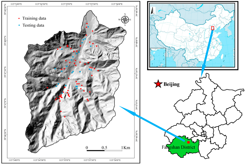
Figure 1.
Geographical position of the Xiqu Gully, Beijing.
The Xiqu Gully was once a colliery. Slag from the coal mining process was left and deposited there. Due to the long-term presence of the coalmine, there is evidence of subsidence and ground fissures in the study area. Subsidence and fissures may be hazards by themselves, but they also have a negative influence on the formation of flash floods. Flash flooding is a phenomenon related to the surface water flow, which is substantially affected by the presence of subsidence and ground fissures. Surface water may reach the groundwater reserves through subsidence and fissures, which can reduce the effects of flash flooding (Figure 2).
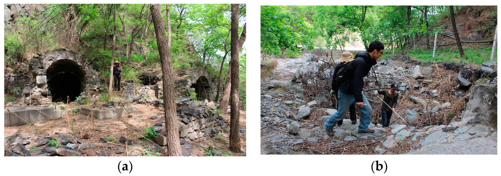
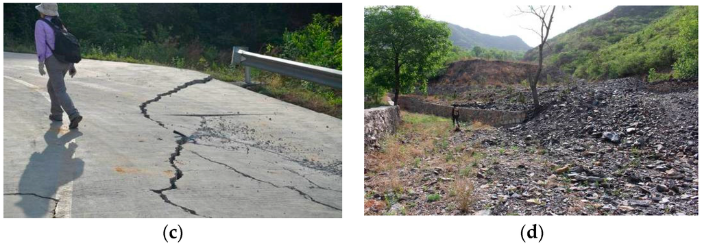
Figure 2.
Field survey: (a) coalmine caves; (b) subsidence; (c) ground fissures and (d) coalmine slag.
2.1. Flash Flood Hazard Inventory
A flash flood hazards inventory map shows the spatial distribution of flash flood hazards in the study area. This is used as the base map for producing a FFHSM. It is necessary to analyze the past records of flash flooding hazards in order to delineate areas that are susceptible to flash flooding hazards. The flash flood hazard inventory map used for this study is mainly a collection of flash flood occurrences on 21 July 2012 and some flash flood hazards occurred in XQG during 2012–2015. The inventory map was developed by first identifying the flash flood hazard locations in XQG using the available documentation and a detailed field survey. Landslides, collapses, erosions, etc. caused by flash flooding were identified through the field survey (Figure 3). Road surfaces experienced lateral erosion due to flash flooding. Farmland terraces in hillsides were destroyed by flash flooding, causing small landslides. Identifying the effects of flash flooding is fairly straightforward. Meanwhile, through interviews with area residents, the authors also identified houses and public facilities that were destroyed by flash floods.
Figure 3.
Flash flood hazards in the field: (a) landslide; (b) roadbed scouring; (c) lateral erosion and (d) ground erosion.
Through the detailed field survey, a total of 85 hazards caused by flash flooding were identified and located on the map. The locations of these 85 flash flood hazards (n = 85) are shown in Figure 1. Previous work suggests the appropriate number of samples that should be used for analysis and validation []. In this analysis, 70% (n = 60) of the hazard locations were selected for training the FFHSM models. The remaining 30% (n = 25) were used as model validation data. The field survey revealed that most vulnerability were roads, residential areas, and dam terraces. Residents in the area had constructed artificial drainage systems. However, due to the rainstorm on 21 July 2012 in Beijing, the drainages were destroyed by flash flooding (Figure 3).
2.2. Conditioning Parameters
In order to generate a model for evaluating the hazard susceptibility, a series of conditioning parameters must be defined [,,]. Various thematic data layers representing flash flooding hazard conditioning parameters, such as elevation, slope, curvature, land use, geology, soil texture, subsidence risk area, stream power index (SPI), topographic wetness index (TWI), and short-term heavy rain, were derived. Determination of the conditioning parameters for flash flooding hazards is important, as they vary widely from one study area to another []. Note that this type of flash flooding assessment should be applicable for this catchment. Thus, the chosen parameters should be representative, reliable, and readily obtained for the study area.
Water flows from higher to lower elevations, and low elevation areas may flood quicker than areas at higher elevation. Flash flooding typically does not occur in high elevation regions []. The elevation of the study area is shown in Figure 4a. Meanwhile, slope and curvature also influence the amount of surface runoff and infiltration []. Flat areas more easily accumulate water (Figure 4b). Curvature is classified into three classes: concave, convex, and flat (Figure 4c). Stream power index (SPI) represents the power of water flow in terms of erosion []. The topographic wetness index (TWI) shows the amount of flow accumulation at any point in a drainage basin and the ability of the water to travel downslope with gravity []. This parameter is related to soil moisture status. Figure 4d,e shows the thematic layers for SPI and TWI, respectively. Elevation, slope, TWI and SPI were classified by the natural breaks method [,,]. SPI and TWI were calculated using the following equations []:
where As is the specific catchment area (m2/m), and β (radian) is the slope gradient (in degrees) [].
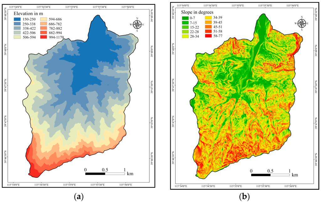
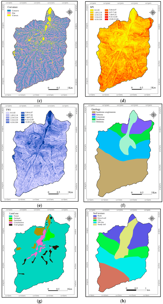
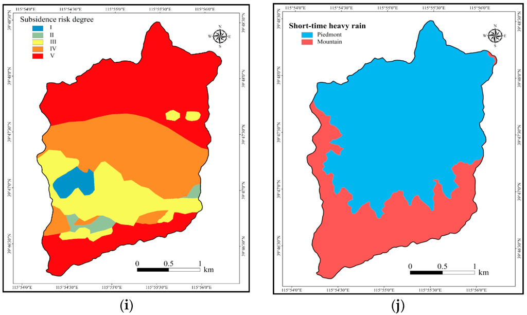
Figure 4.
Input thematic layers: (a) elevation; (b) slope; (c) curvature; (d) SPI; (e) TWI; (f) geology; (g) land use; (h) soil texture; (i) subsidence risk area and (j) short-term heavy rain.
Five geology classes were used to create the geology map: Limestone, dolomite, siltstone, sandstone intercalated with conglomerate, and sandstone (Figure 4f). The land use data for the XQG provided by the Beijing Institute of Geology is shown in Figure 4g. Land use influences water infiltration. In the study area, there are five land use types: forest, orchard, farmland, coal gangue, and construction areas. Forest, orchard, and farmland favor infiltration. Coal gangue and construction areas support surface flow. The soil layer was produced using five soil textures that can be seen in Figure 4h. Sandy soil is found in the villages, which is where most of the flash flooding hazard occurred in the catchment. Because the XQG used to be a coal mining area, there is the potential for subsidence in the study area. Zhang [] proposed a method to predict the potential mining subsidence risk and categorized five zones of risk in the Xishan area of Beijing. The XQG is located within Xishan. Figure 4i displays the risk zoning results. Flash flooding is a type of runoff along the ground surface. In the most dangerous subsidence areas, runoff easily flows into the groundwater through ground fissures. In these instances, the susceptibility to flash flooding in the subsidence area becomes very low.
Rainfall plays a very important role in the occurrence of flash flood. Flash flood is caused by heavy or excessive rainfall in a short period of time, generally less than six hours. Brooks [] considered that flash flooding is frequently associated with heavy precipitation occurring over a short period of time. He believed that the hourly precipitation dataset (HPD) could be useful for observing and defining the threat of flash flooding. HPD is used to develop a climatology of heavy rains on timescales of 3 h or less. Hourly precipitation data collected from 187 weather stations in Beijing between 2006 and 2010 were used in this study. Spatially, in the western mountainous area of Beijing, the frequency of short-term heavy rains (STHR) (defined here as ≥20 mm/h) is very low in high elevation areas. The piedmont and the plains are the more common locations for STHR, which have a greater rainfall accumulation than that of higher elevation areas []. The XQG is a small-scale catchment located in the western mountainous area. Differences in elevation within the XQG are greater than 1000 m, and the urban district sees high incidences of STHR, where the four villages are located []. Regions where elevation is more than 500 m are considered mountainous zones in China. Based on this factor and the rain gauge data in XQG, we divided STHR data into two classes: (1) 150 m–500 m; and (2) 500 m–1170 m. The first class is considered piedmont and the second class is referred to as mountainous (Figure 4j).
3. Data Collection
Field surveys and prior research were used to identify the relationship between the occurrence of flash flooding hazards and the conditioning parameters. The 85 flood locations were investigated and mapped in the study area at a scale of 1:10,000. A Digital Elevation Model (DEM) with 2.5 m × 2.5 m resolution covers an area of 7.98 km2 and was produced using the 5 m interval contours from a geomorphologic map generated using Geographic Information System (GIS). The DEM is the ideal source from which to derive topographic parameters of elevation, slope, curvature, SPI, and TWI. The DEM and its derivatives play a major role in determining which areas are susceptible to flood occurrence []. The geology parameter was obtained using a geological map of Beijing, which has a scale of 1:10,000. The land use parameter was extracted from remotely-sensed imagery. Both the land use data and soil texture data were provided by the Beijing Institute of Geology. The subsidence risk level parameter was obtained from Zhang []. Short-term heavy rain data were collected from 187 weather stations in Beijing during 2006–2010 and summarized by Wang [].
Because the results depend on the classification of different parameters, this study attempted different manual parameter classification schemes for elevation, slope, TWI, and SPI. Elevation was divided into ten classes: (1) 150 m–250 m; (2) 250 m–350 m; (3) 350 m–450 m; (4) 450 m–550 m; (5) 550 m–650 m; (6) 650 m–750 m; (7) 750 m–850 m; (8) 850 m–950 m; (9) 950 m–1050 m; and (10) 1050–1170 m. The slope was reclassified into eight classes: (1) 0°–10°; (2) 10°–20°; (3) 20°–30°; (4) 30°–40°; (5) 40°–50°; (6) 50°–60°; (7) 60°–70°; and (8) 70°–77.65°. Both SPI and TWI were reclassified into ten classes: (1) 0–1; (2) 1–2; (3) 2–3; (4) 3–4; (5) 4–5; (6) 5–6; (7) 6–7; (8) 7–8; (9) 8–9; and (10) >9.
4. Methods
4.1. Frequency Ratio
The Frequency ratio (FR) model was adopted to generate a FFHSM in this study. A simple geospatial assessment tool for understanding the probabilistic relationship between dependent and independent variables, including spatial datasets with multiple classification levels, can be applied to the FR model []. This approach can be described as an FR index that represents the quantitative relationship between flash flooding hazards occurrence and different conditioning parameters. It is expressed based on Equation (3):
where FFHSI is the flash flood hazard susceptibility index and FR is the frequency ratio for each parameter. The FR can be defined as the ratio of the area where flash flooding hazards may occur to the total study area, or the ratio of the probability of a flash flood hazard occurrence to a non-occurrence as shown in Equation (4) []:
where A is the number of pixels with a flash flooding hazard for each class of each parameter; B is the total number of pixels with flash flooding hazards in study area; M is the number of pixels for each class of the parameter; and N is total number of pixels in the study area.
In this analysis, if the FR value is greater than 1, it means there is a stronger correlation, whereas a value of less than 1 means there is a weaker correlation. The spatial relationship between each flash flood conditioning parameter and flash flooding hazards derived from the frequency ratio model is shown in Table 1. The manual parameter classification for elevation, slope, TWI, and SPI calculated by FR are shown in Table 2.

Table 1.
Distribution of the training pixels.
Table 2.
Distribution of the training pixels in manual classification schemes.
In Table 1, FR is the flash flooding hazard susceptibility index that was calculated by Equation (4). A represents the number of flash flooding hazards for each parameter. B represents the total number of flash flooding hazards across all 60 hazard locations that were selected as training data. M represents the number of pixels for each parameter, and N represents the number of pixels in the study domain.
In order to produce a flash flooding hazard susceptibility map, the FFHSI was calculated by summing each weighted factor using the following equation:
Thus, a flash flooding hazard susceptibility map was produced using the FR model.
4.2. Statistical Index
The statistical index (SI) approach was introduced by Van Westen []. It is a bivariate statistical analysis that has been widely used in many studies [,,]. In the statistical index method, the weighted value for each categorical unit is defined as the natural logarithm of the flash flooding hazard density in any class divided by the flash flooding hazard density for the entire study area. This method is based on the distribution of flash flood hazards across each class. It can be expressed by the formula:
where Wij is the weight given to the i-th class of the j-th parameter. Dij is the flash flooding hazard density within the i-th class of the j-th parameter. D is the total flash flooding hazard density within the study area. Nij is the number of pixels with flash flooding hazard in the i-th class of the j-th parameter. Mij is the number of pixels in the i-th class of the j-th parameter. N is the total number of flash flooding hazards in the study area. M is the total number of pixels in the study area. Since the natural logarithm (ln) is not defined, the weighting value (Wij) can only be calculated for classes that contain flash flooding hazards.
where FFHSI, Wij and n represent the flash flood hazard susceptibility index, the weighting values of the i-th class of the j-th parameter using the SI model and the number of conditioning parameters, respectively.
Table 1 shows the spatial relationship between each conditioning parameter and flash flooding hazards using the statistical index model. In Table 1, Wij (SI) shows the flash flooding hazard susceptibility index using the statistical index method. Nij represents the number of flash flooding hazards in the i-th class of the j-th parameter. Mij represents the number of pixels in the i-th class of the j-th parameter. N is the total number of flash flooding hazards, out of the 60 hazard locations. M represents the number of pixels in the domain. Because there are no flash flooding hazards in the study area between 994 m and 1170 m elevation, the Wij (SI) for this class is set to −1 to indicate the extremely low possibility of flash flood hazard occurrence [].
5. Results and Discussion
5.1. Application of the Frequency Ratio Model
Application of the frequency ratio model found that most flash flooding hazards are located at elevations of 150 m–422 m. Elevation class 150 m–250 m has the highest FR value of 2.52, followed by 250 m–338 m, and 338 m–422 m. Elevations higher than 506 m had the lowest frequency ratio (0.00), agreeing with earlier work that found that flooding is unlikely in high elevation regions []. In the case of slope, it could be seen that the classes 0°–7°, 7°–15°, and 15°–22° had higher FR values, followed by 34°–39°. Flooding was not possible at slopes higher than 51°. For the curvature parameter, flat areas proved to be the most prone to flooding with the highest FR value of 2.14. The convex and concave classes had the lowest FR values of 0.94 and 0.89, respectively. As for the SPI parameter, the class 0–1.03 had the highest FR value, followed by classes 1.03–2.14 and 2.14–3.16. The FR values of SPI generally decreased as the value of SPI decreased. FR values for the TWI classes showed a general trend that increased with higher TWI values in the range of 0–5.15. For the geology parameter, the dolomite class had the highest FR value of 2.78, indicating high susceptibility in this area, followed by sandstone conglomerate and limestone. As for the land use parameter, the FR values for coal gangue and construction areas were 5.67 and 3.77, respectively, as these two classes support the overland flow of water. Forest, orchard, and farmland classes are more likely to store water in the soil. The lowest FR value of 0.63 belonged to the forest class. For soil texture, results found that sandy soil and silt clay have the highest FR values (2.40 and 1.14, respectively), implying that these characteristics are favorable for flash flooding hazards. Regarding subsidence risk, classes I, II and III have the highest FR values (1.15, 1.37 and 0.84, respectively). This implies that the higher the subsidence risk, the lower the potential for flash flooding hazards. When it comes to short-term heavy rain, the piedmont and mountainous areas both have hazard susceptibility (2.79 and 1.39, respectively).
Based on Equation (5), the FR flash flooding hazards susceptibility map is shown in Figure 5a. The map was divided into five susceptibility classes (very low, low, moderate, high, and very high) using the natural breaks method []. Table 3 displays the FFHSM for the five classes are 2.53, 2.66, 1.30, 0.94 and 0.56 km2.
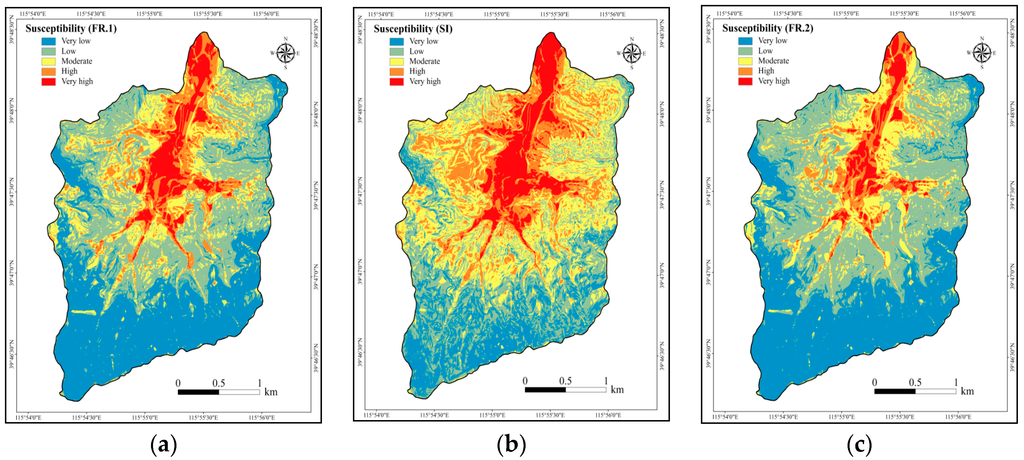
Figure 5.
Flash flood hazard susceptibility using (a) Frequency Ratio-natural breaks method (FR.1) (b) Statistical Index-natural breaks (SI) and (c) Frequency Ratio-manual classification (FR.2).
Table 3.
Flash flood hazard susceptibility classification in the Xiqu Gully.
5.2. Application of the Statistical Index Model
For the elevation parameter, classes 150 m–250 m, 250 m–338 m, and 338 m–422 m had positive SI values (0.92, 0.38 and 0.36, respectively). When elevations were higher than 422 m, the SI values became negative. In the case of the slope angle parameter, 7°–15° had the highest positive value (1.11), indicating the highest probability of flash flooding hazards occurrence. The SI value continued to be positive for slope angle class greater than 15°, but when slope angle was greater than 22°, SI values were negative. For the curvature parameter, the only positive SI value occurred in the flat class (0.76), while the convex and concave class values were negative (−0.06 and −0.12, respectively). In the case of SPI, the class 0–1.03 had a positive SI value, meaning this range is more susceptible to flash flooding hazards. As for the TWI parameter, SI values were negative between classes 0–1.53, 1.53–1.94, and 1.94–2.80. The highest value (1.53) was for class 4.08–5.15, meaning that as TWI reached 5.15, SI only increased. SI values were positive for dolomite and siltstone geological areas, while limestone, sandstone conglomerate, and siltstone classes were negative (−0.09, 0.35 and −0.29, respectively). As Table 1 shows, SI values for the land use classes were as follows: coal gangue (1.74), construction (1.33), farmland (1.16), orchard (0.39) and forest (−0.46). Among the land use classes, only forest had a negative effect on flash flooding hazards. In the case of soil texture, sandy soil (0.88), silt clay (0.13), and rock (0.02) classes had positive SI values, while clay (−0.70) and gravel soil (−1.73) had negative values. For subsidence risk, level II had the highest SI value (0.31), followed by level III (0.14), and level I (−0.18). Levels IV and V had the highest risk of subsidence, an overall negative impact on the occurrence of flash flooding hazards. SI values were as follows in terms of short-term heavy rain: piedmont (0.37) and mountainous (−2.97).
Based on Equation (7), the SI flash flooding hazards susceptibility map is shown in Figure 5b. Five susceptibility categories were created using the natural breaks method []: very low (−8.51–−4.65), low (−4.65–−1.98), moderate (−1.98–0.76), high (0.76–4.06), and very high (4.06–9.40). The five categories areas were 1.25, 2.10, 2.31, 1.49 and 0.84 km2.
5.3. Validation
It is essential to verify the predictive capabilities of the FFHSM. Both models should be validated to be scientifically rigorous []. This study used success and prediction rate methods to validate the two FFHSMs by comparing predicted hazard areas to existing hazard locations []. A total of 85 flood hazards were generated and located on the map. Previous work suggests that 70% (n = 60) of the flooded hazard locations should be randomly selected for the training database. Meanwhile, an area under curve (AUC) method evaluated the prediction capabilities of the three classification methods. The AUC calculated success and prediction rate percentages of each model and was obtained using both the training data and the testing data. The larger the AUC value, the better the prediction ability of the model. Figure 6a displays accuracy rates of 86.61%, 83.35%, and 78.52% for the FR-natural breaks (FR.1), SI-natural breaks, and FR-manual (FR.2) classification methods, respectively. The associated prediction accuracy rates were 83.69%, 81.22%, and 74.23%, respectively. These results show that both FR and SI were fairly good at predicting the flooding hazard susceptibility for the XQG, with FR being slightly better than SI, and the FR natural breaks classification performing better than FR manual classification.
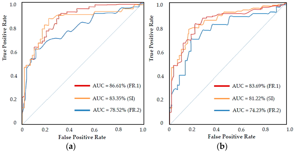
Figure 6.
Success and prediction rate curves using Frequency Ratio-natural break (FR.1), Frequency Ratio-manual classification (FR.2) and Statistical Index-natural breaks (SI): (a) success rate curve (b) prediction rate curve.
5.4. Discussion
Figure 5a,b show that the residential areas of the XQG are the most high risk vulnerable. Areas of very high and high susceptibility accounted for 18.75% and 29.16% of the whole catchment, based on the FR-natural breaks method and SI-natural breaks method, respectively. People who live in these areas should be aware of the potential hazards caused by flash flooding, because all four villages are located in highly susceptible areas. Farmland, orchards, and some forest classes were found in vulnerable areas, mostly in low elevation and flat. Lower elevation areas are more susceptible to flooding []. Slope also influenced the amount of surface runoff and infiltration, consistent with earlier findings []. People who reside in very high and high susceptibility areas should pay attention to weather forecasts for heavy rain and evacuate in advance. Areas of moderate susceptibility accounted for 16.29% and 28.98% of the whole study area using FR-natural breaks method and SI-natural breaks methods, respectively. These were primarily found in middle to high elevations.
As Figure 5a,b show, very low and low susceptibility classes are mainly located in high elevation and high slope angle areas. However, the susceptibility map produced by FR was different from that of SI. Comparing the two maps, classes with low susceptibility in FR map had higher susceptibility in the SI map. The FR method found that subsidence risk had a negative influence on the susceptibility of flash flooding hazards; thus these areas were classified as very low and low susceptibility. In contrast, there was no obvious evidence that subsidence risk areas played a role in flash flooding susceptibility using the SI method. The SI map shows some moderate susceptibility in high elevation areas, mainly located in the channel where water flowed. However, the role of subsidence and ground fissures cannot be ignored in the XQG. In other words, both the FR and SI maps are able to inform the people in the XQG of how to prevent damage and escape from flash flooding hazards, but the FR method appears to reflect the actual situation of the XQG considering the subsidence and ground fissure features.
In this study, we also used a manual classification scheme. The results were different from those of the natural breaks classification method. These are shown in Figure 5c, where high elevation and high slope angle areas were classified correct into low and very low susceptibility areas. However, compared with Figure 5a, some of the residential areas were not classified into the correct susceptibility category. Residential areas should receive the most attention. In Table 3, areas of high and very high susceptibility account for 12.98% of the total study area, which is much less than the other two methods (18.75% and 29.16%). Manual classification method is a subjective methodology, while the natural breaks classification method avoids this pitfall. Natural breaks classification is a data clustering method designed to determine the best arrangement of values into different classes. This is done by seeking to minimize each class’s average deviation from the class mean, while maximizing each class’s deviation from the means of the other classes. In other words, the method seeks to reduce the variance within classes and maximize the variance between classes [,]. Thus, natural breaks method is more appropriate for the classification of parameters in FFHSM using an FR method.
If this method was applied to another catchment or a larger study area, the selection of the appropriate conditioning parameters is essential. The conditioning parameters should reflect the characteristics of the catchment based on field survey data collection and other case studies with similar characteristics. For example, because the XQG is a catchment with coalmine subsidence, the subsidence risk level must be taken into consideration. And as this catchment has elevation differences >1000 m, precipitation should be considered in different way. Because the XQG is a small-scale catchment, and there are several rain gauges that being set in the catchment. So the rainfall data collected and analyzed more accuracy. As for large-scale catchment, the annual rainfall data or summer rainfall data can be used as a parameter for FFHSM. The rainfall data can be obtained from rainfall distribution map. And the other parameters, such as elevation, slope, curvature, land use, geology, soil texture, subsidence risk area, stream power index (SPI) and topographic wetness index (TWI), should also be taken into consideration. However, the accuracy of the conditioning parameters in large-scale study area cannot be as high as that in small-scale study area. And the results prediction accuracy would be decreased. Therefore, if we apply these two methods on large-scale study area, the accuracy of the thematic layers must be obtained accurately in case of decreasing prediction accuracy.
Areas where people live were mostly located in lower elevations and flat areas. These areas suffered from high and very high susceptibility levels of flash flooding hazards. People who reside there should consider constructing protective barriers for flash flooding. Additionally, subsidence areas should also be a focus because they are prone to sink or collapse during flood events.
6. Conclusions
In this study, two GIS-based models, frequency ratio (FR) and statistical index (SI), were applied to generate flash flood hazard susceptibility maps (FFHSM) for the XQG in Beijing, China, and their performance was compared. Input parameters were classified using the natural breaks method and a manual classification method. The results of the two classification methods were tested using the FR model. The area under the curve (AUC) was used as a validation method.
Based on detailed field survey results, this study selected ten conditioning parameters to generate the FFHSM. Conditioning parameters included elevation, slope, curvature, land use, geology, soil texture, subsidence risk level, stream power index (SPI), topographic wetness index (TWI), and short-term heavy rain. A total of 85 flash flooding hazard locations were surveyed in the field and prepared in GIS software for the models, where 70% (60 flooded locations) were used randomly for training and building the FFHSM models. The remaining 30% (25 flooded locations) were used for model validation. FFHSMs were produced from map index values for each conditioning parameter calculated using SI and FR models (with the latter using two different classification methods). The final results were plotted in ArcGIS.
The maps produced by the two models were divided into five classes, including very low, low, moderate, high and very high flash flooding hazard susceptibility. AUC results of FR and SI models showed that both models performed well in training and prediction. The susceptibility maps generated by the two approaches were reliable and applicable, able to assist government and planners to take proper action in order to prevent flash flooding hazards. Based on the field survey and map products, this study found that the FR model was more appropriate for guiding management of the XQG. Because subsidence and ground fissures are characteristics of XQG, the FR method may better reflect the actual flash flood hazard susceptibility. The FR method also showed higher accuracy in success and prediction rates than SI.
This study also compared different classification schemes to classify the values for each conditional parameter and checked the impacts on the results. Of the ten parameters, four parameters were classified by a natural breaks method and a manual classification method: elevation, slope, TWI, and SPI. Results from the two classification methods were vastly different. Using only manual classification, residential areas were not classified into the correct susceptibility category. As an objective method, on the other hand, the natural breaks method seeks to reduce the variance within classes and maximize the variance between classes. Consequently, the natural breaks method was more appropriate than manual classification for FFHSM parameters using an FR model.
Acknowledgments
This work was supported by the State Key Program of National Natural Science of China (Grant No. 41330636). Natural Science Foundations of China (Grant No. 41402243). Beijing science and technology project (Grant No. Z141100003614052). Graduate Innovation Fund of Jilin University (2016208). Thanks to anonymous reviewers for their valuable feedback on the manuscript.
Author Contributions
Chen Cao and Peihua Xu have equal contribution to data analysis and manuscript writing. Jianping Chen proposed the main structure of this study. Yihong Wang is the project provider. Lianjing Zheng and Cencen Niu provided useful advice and revised the manuscript. All authors read and approved the final manuscript.
Conflicts of Interest
The authors declare no conflict of interest.
References
- Guzzetti, F.; Stark, C.P.; Salvati, P. Evaluation of flood and landslide risk to the population of Italy. Environ. Manag. 2005, 36, 15–36. [Google Scholar] [CrossRef] [PubMed]
- Penning-Rowsell, E.; Floyd, P.; Ramsbottom, D.; Surendran, S. Estimating injury and loss of life in floods: A deterministic framework. Nat. Hazards 2005, 36, 43–64. [Google Scholar] [CrossRef]
- Salvati, P.; Bianchi, C.; Rossi, M.; Guzzetti, F. Societal landslide and flood risk in Italy. Nat. Hazard Earth Syst. Sci. 2010, 10, 465–483. [Google Scholar] [CrossRef]
- Du, J.; Fang, J.; Xu, W.; Shi, P.J. Analysis of dry/wet conditions using the standardized precipitation index and its potential usefulness for drought/flood monitoring in Hunan province, China. Stoch. Environ. Res. Risk Assess. 2013, 27, 377–387. [Google Scholar] [CrossRef]
- Tehrany, M.S.; Pradhan, B.; Jebur, M.N. Flood susceptibility analysis and its verification using a novel ensemble support vector machine and frequency ratio method. Stoch. Environ. Res. Risk Assess. 2015, 29, 1149–1165. [Google Scholar] [CrossRef]
- Grimaldi, S.; Petroselli, A.; Arcangeletti, E.; Nardi, F. Flood mapping in ungauged basins using fully continuous hydrologic-hydraulic modeling. J. Hydrol. 2013, 487, 39–47. [Google Scholar] [CrossRef]
- Zhang, D.W.; Quan, J.; Zhang, H.B.; Wang, F.; Wang, H.; He, X.Y. Flash flood hazard mapping: A pilot case study in Xiapu River Basin, China. Water Sci. Eng. 2015, 8, 195–204. [Google Scholar] [CrossRef]
- Perucca, L.P.; Angilieri, Y.E. Morphometric characterization of del molle basin applied to the evaluation of flash floods hazard, Iglesia department, San Juan, Argentina. Quat. Int. 2011, 233, 81–86. [Google Scholar] [CrossRef]
- Bajabaa, S.; Masoud, M.; Al-Amri, N. Flash flood hazard mapping based on quantitative hydrology, geomorphology and gis techniques (case study of Wadi Al-Lith, Saudi Arabia). Arab. J. Geosci. 2014, 7, 2469–2481. [Google Scholar] [CrossRef]
- Youssef, A.M.; Pradhan, B.; Sefry, S.A. Flash flood susceptibility assessment in jeddah city (Kingdom of Saudi Arabia) using bivariate and multivariate statistical models. Environ. Earth Sci. 2016, 75, 12. [Google Scholar] [CrossRef]
- Pramanik, N.; Panda, R.K.; Sen, D. Development of design flood hydrographs using probability density functions. Hydrol. Process. 2010, 24, 415–428. [Google Scholar] [CrossRef]
- Serinaldi, F.; Grimaldi, S. Synthetic design hydrographs based on distribution functions with finite support. J. Hydrol. Eng. 2011, 16, 434–446. [Google Scholar] [CrossRef]
- Grimaldi, S.; Petroselli, A.; Serinaldi, F. A continuous simulation model for design-hydrograph estimation in small and ungauged watersheds. Hydrol. Sci. J. 2012, 57, 1035–1051. [Google Scholar] [CrossRef]
- Hsieh, L.S.; Hsu, M.H.; Li, M.H. An assessment of structural measures for flood-prone lowlands with high population density along the Keelung River in Taiwan. Nat. Hazards 2006, 37, 133–152. [Google Scholar] [CrossRef]
- Laforce, S.; Simard, M.C.; Leconte, R.; Brissette, F. Climate change and floodplain delineation in two southern Quebec River Basins. J. Am. Water Resour. Assoc. 2011, 47, 785–799. [Google Scholar] [CrossRef]
- Manfreda, S.; Nardi, F.; Samela, C.; Grimaldi, S.; Taramasso, A.C.; Roth, G.; Sole, A. Investigation on the use of geomorphic approaches for the delineation of flood prone areas. J. Hydrol. 2014, 517, 863–876. [Google Scholar] [CrossRef]
- Tucker, G.E.; Whipple, K.X. Topographic outcomes predicted by stream erosion models: Sensitivity analysis and intermodel comparison. J. Geophys. Res. Solid Earth 2002, 107, 1–16. [Google Scholar] [CrossRef]
- McGlynn, B.L.; Seibert, J. Distributed assessment of contributing area and riparian buffering along stream networks. Water Resour. Res. 2003, 39, 1082. [Google Scholar] [CrossRef]
- Dodov, B.A.; Foufoula-Georgiou, E. Floodplain morphometry extraction from a high-resolution digital elevation model: A simple algorithm for regional analysis studies. IEEE Geosci. Remote Sens. 2006, 3, 410–413. [Google Scholar] [CrossRef]
- Petroselli, A.; Alvarez, A.F. The flat-area issue in digital elevation models and its consequences for rainfall-runoff modeling. Gisci. Remote Sens. 2013, 27, 1201–1215. [Google Scholar] [CrossRef]
- Cloke, H.L.; Pappenberger, F. Ensemble flood forecasting: A review. J. Hydrol. 2009, 375, 613–626. [Google Scholar] [CrossRef]
- Biswajeet, P.; Mardiana, S. Flood hazrad assessment for cloud prone rainy areas in a typical tropical environment. Disaster Adv. 2009, 2, 7–15. [Google Scholar]
- Pradhan, B.; Hagemann, U.; Tehrany, M.S.; Prechtel, N. An easy to use arcmap based texture analysis program for extraction of flooded areas from terrasar-x satellite image. Comput. Geosci. UK 2014, 63, 34–43. [Google Scholar] [CrossRef]
- Kim, E.S.; Choi, H.I. A method of flood severity assessment for predicting local flood hazards in small ungauged catchments. Nat. Hazards 2015, 78, 2017–2033. [Google Scholar] [CrossRef]
- Sanyal, J.; Lu, X.X. Application of remote sensing in flood management with special reference to monsoon asia: A review. Nat. Hazards 2004, 33, 283–301. [Google Scholar] [CrossRef]
- Balogun, A.L.; Matori, A.N.; Hamid-Mosaku, A.I. A fuzzy multi-criteria decision support system for evaluating subsea oil pipeline routing criteria in east malaysia. Environ. Earth Sci. 2015, 74, 4875–4884. [Google Scholar] [CrossRef]
- Tehrany, M.S.; Pradhan, B.; Jebur, M.N. Spatial prediction of flood susceptible areas using rule based decision tree (dt) and a novel ensemble bivariate and multivariate statistical models in GIS. J. Hydrol. 2013, 504, 69–79. [Google Scholar] [CrossRef]
- Mukerji, A.; Chatterjee, C.; Raghuwanshi, N.S. Flood forecasting using ann, neuro-fuzzy, and neuro-ga models. J. Hydrol. Eng. 2009, 14, 647–652. [Google Scholar] [CrossRef]
- Pulvirenti, L.; Pierdicca, N.; Chini, M.; Guerriero, L. An algorithm for operational flood mapping from synthetic aperture radar (sar) data using fuzzy logic. Nat. Hazard Earth Syst. Sci. 2011, 11, 529–540. [Google Scholar] [CrossRef]
- Tehrany, M.S.; Pradhan, B.; Jebur, M.N. Flood susceptibility mapping using a novel ensemble weights-of-evidence and support vector machine models in gis. J. Hydrol. 2014, 512, 332–343. [Google Scholar] [CrossRef]
- Campolo, M.; Soldati, A.; Andreussi, P. Artificial neural network approach to flood forecasting in the river arno. Hydrol. Sci. J. 2003, 48, 381–398. [Google Scholar] [CrossRef]
- Kia, M.B.; Pirasteh, S.; Pradhan, B.; Mahmud, A.R.; Sulaiman, W.N.A.; Moradi, A. An artificial neural network model for flood simulation using gis: Johor River Basin, Malaysia. Environ. Earth Sci. 2012, 67, 251–264. [Google Scholar] [CrossRef]
- Tiwari, M.K.; Chatterjee, C. Uncertainty assessment and ensemble flood forecasting using bootstrap based artificial neural networks (Banns). J. Hydrol. 2010, 382, 20–33. [Google Scholar] [CrossRef]
- Rahmati, O.; Pourghasemi, H.R.; Zeinivand, H. Flood susceptibility mapping using frequency ratio and weights-of-evidence models in the Golastan province, Iran. Geocarto Int. 2016, 31, 42–70. [Google Scholar] [CrossRef]
- Nandi, A.; Mandal, A.; Wilson, M.; Smith, D. Flood hazard mapping in jamaica using principal component analysis and logistic regression. Environ. Earth Sci. 2016, 75, 465. [Google Scholar] [CrossRef]
- Wang, Q.Q.; Li, W.P.; Yan, S.S.; Wu, Y.L.; Pei, Y.B. Gis based frequency ratio and index of entropy models to landslide susceptibility mapping (Daguan, China). Environ. Earth Sci. 2016, 75, 780. [Google Scholar] [CrossRef]
- Zhang, Z.W.; Yang, F.; Chen, H.; Wu, Y.L.; Li, T.; Li, W.P.; Wang, Q.Q.; Liu, P. Gis-based landslide susceptibility analysis using frequency ratio and evidential belief function models. Environ. Earth Sci. 2016, 75, 948. [Google Scholar] [CrossRef]
- Wu, Y.L.; Li, W.P.; Wang, Q.Q.; Liu, Q.Q.; Yang, D.D.; Xing, M.L.; Pei, Y.B.; Yan, S.S. Landslide susceptibility assessment using frequency ratio, statistical index and certainty factor models for the Gangu County, China. Arab. J. Geosci. 2016, 9, 84. [Google Scholar] [CrossRef]
- Zhao, C.X.; Chen, W.; Wang, Q.Q.; Wu, Y.L.; Yang, B. A comparative study of statistical index and certainty factor models in landslide susceptibility mapping: A case study for the Shangzhou district, Shaanxi province, China. Arab. J. Geosci. 2015, 8, 9079–9088. [Google Scholar] [CrossRef]
- Bui, D.T.; Lofman, O.; Revhaug, I.; Dick, O. Landslide susceptibility analysis in the Hoa Binh province of Vietnam using statistical index and logistic regression. Nat. Hazards 2011, 59, 1413–1444. [Google Scholar] [CrossRef]
- Ohlmacher, G.C.; Davis, J.C. Using multiple logistic regression and gis technology to predict landslide hazard in Northeast Kansas, USA. Eng. Geol. 2003, 69, 331–343. [Google Scholar] [CrossRef]
- Jebur, M.N.; Pradhan, B.; Tehrany, M.S. Manifestation of lidar-derived parameters in the spatial prediction of landslides using novel ensemble evidential belief functions and support vector machine models in GIS. IEEE J. Sel. Top. Appl. Earth Remote Sens. 2015, 8, 674–690. [Google Scholar] [CrossRef]
- Tehrany, M.S.; Pradhan, B.; Mansor, S.; Ahmad, N. Flood susceptibility assessment using GIS-based support vector machine model with different kernel types. Catena 2015, 125, 91–101. [Google Scholar] [CrossRef]
- Elkhrachy, I. Flash flood hazard mapping using satellite images and gis tools: A case study of najran city, kingdom of Saudi Arabia (KSA). Egypt. J. Remote Sens. Space Sci. 2015, 18, 261–278. [Google Scholar] [CrossRef]
- Botzen, W.J.W.; Aerts, J.C.J.H.; van den Bergh, J.C.J.M. Individual preferences for reducing flood risk to near zero through elevation. Mitig. Adapt. Strateg. Glob. Chang. 2013, 18, 229–244. [Google Scholar] [CrossRef]
- Kazakis, N.; Kougias, I.; Patsialis, T. Assessment of flood hazard areas at a regional scale using an index-based approach and analytical hierarchy process: Application in Rhodope-Evros region, Greece. Sci. Total Environ. 2015, 538, 555–563. [Google Scholar] [CrossRef] [PubMed]
- Jebur, M.N.; Pradhan, B.; Tehrany, M.S. Optimization of landslide conditioning factors using very high-resolution airborne laser scanning (lidar) data at catchment scale. Remote Sens. Environ. 2014, 152, 150–165. [Google Scholar] [CrossRef]
- Gokceoglu, C.; Sonmez, H.; Nefeslioglu, H.A.; Duman, T.Y.; Can, T. The 17 march 2005 Kuzulu Landslide (Sivas, Turkey) and landslide-susceptibility map of its near vicinity. Eng. Geol. 2005, 81, 65–83. [Google Scholar] [CrossRef]
- Falaschi, F.; Giacomelli, F.; Federici, P.R.; Puccinelli, A.; Avanzi, G.D.; Pochini, A.; Ribolini, A. Logistic regression versus artificial neural networks: Landslide susceptibility evaluation in a sample area of the Serchio River Valley, Italy. Nat. Hazards 2009, 50, 551–569. [Google Scholar] [CrossRef]
- Pourghasemi, H.R.; Pradhan, B.; Gokceoglu, C. Application of fuzzy logic and analytical hierarchy process (ahp) to landslide susceptibility mapping at Haraz Watershed, Iran. Nat. Hazards 2012, 63, 965–996. [Google Scholar] [CrossRef]
- Cao, C.; Wang, Q.; Chen, J.; Ruan, Y.; Zheng, L.; Song, S.; Niu, C. Landslide susceptibility mapping in vertical distribution law of precipitation area: Case of the Xulong Hydropower station Reservoir, Southwestern China. Water 2016, 8, 270. [Google Scholar] [CrossRef]
- Regmi, N.R.; Giardino, J.R.; Vitek, J.D. Modeling susceptibility to landslides using the weight of evidence approach: Western Colorado, USA. Geomorphology 2010, 115, 172–187. [Google Scholar] [CrossRef]
- Zhang, C.M. Subsidence Features and Risk Prediction in Coalmine Goafs: A Case Study of the Xishan Area in Beijing; Institute of Geology, China Earthquake Administration: Beijing, China, 2009. [Google Scholar]
- Brooks, H.E.; Stensrud, D.J. Climatology of heavy rain events in the United States from hourly precipitation observations. Mon. Weather Rev. 2000, 128, 1194–1201. [Google Scholar]
- Wang, G.; Wang, L. Temporal and spatial distribution of short-time heavy rain of Beijing in summer. Torrential Rain Disasters 2013, 32, 276–279. [Google Scholar]
- Pradhan, B. Groundwater potential zonation for basaltic watersheds using satellite remote sensing data and GIS techniques. Cent. Eur. J. Geosci. 2009, 1, 120–129. [Google Scholar] [CrossRef]
- Laxton, J.L. Geographic information systems for geoscientists—Modelling with GIS—Bonhamcarter, GF. Int. J. Geogr. Inf. Syst. 1996, 10, 355–356. [Google Scholar] [CrossRef]
- Oztekin, B.; Topal, T. GIS-based detachment susceptibility analyses of a cut slope in Limestone, Ankara-Turkey. Environ. Geol. 2005, 49, 124–132. [Google Scholar] [CrossRef]
- Pourghasemi, H.R.; Moradi, H.R.; Aghda, S.M.F. Landslide susceptibility mapping by binary logistic regression, analytical hierarchy process, and statistical index models and assessment of their performances. Nat. Hazards 2013, 69, 749–779. [Google Scholar] [CrossRef]
- Zhang, G.; Cai, Y.; Zheng, Z.; Zhen, J.; Liu, Y.; Huang, K. Integration of the statistical index method and the analytic hierarchy process technique for the assessment of landslide susceptibility in Huizhou, China. Catena 2016, 142, 233–244. [Google Scholar] [CrossRef]
- Feizizadeh, B.; Blaschke, T. GIS-multicriteria decision analysis for landslide susceptibility mapping: Comparing three methods for the Urmia Lake Basin, Iran. Nat. Hazards 2013, 65, 2105–2128. [Google Scholar] [CrossRef]
- Zare, M.; Pourghasemi, H.R.; Vafakhah, M.; Pradhan, B. Landslide susceptibility mapping at vaz watershed (Iran) using an artificial neural network model: A comparison between multilayer perceptron (mlp) and radial basic function (rbf) algorithms. Arab. J. Geosci. 2013, 6, 2873–2888. [Google Scholar] [CrossRef]
- Jenks, G.F. Visualizing statistical distributions and generalizing process. Ann. Assoc. Am. Geogr. 1967, 57, 179–179. [Google Scholar]
- Jenks, G.F.; Caspall, F.C.; Williams, D.L. Error factor in statistical mapping. Ann. Assoc. Am. Geogr. 1969, 59, 186–187. [Google Scholar]
© 2016 by the authors; licensee MDPI, Basel, Switzerland. This article is an open access article distributed under the terms and conditions of the Creative Commons Attribution (CC-BY) license (http://creativecommons.org/licenses/by/4.0/).