Article

Evaluating the Potential of Variable Renewable Energy for a Balanced Isolated Grid: A Japanese Case Study

Research Institute of Science for Safety and Sustainability, National Institute of Advanced Industrial Science and Technology, 16-1 Onogawa, Tsukuba 305-8569, Japan
*
Author to whom correspondence should be addressed.
Sustainability 2017, 9(1), 119; https://doi.org/10.3390/su9010119
Submission received: 30 November 2016 / Revised: 3 January 2017 / Accepted: 9 January 2017 / Published: 14 January 2017
(This article belongs to the Special Issue Sustainable Electric Power Systems Research)

Abstract

:
There is a global push to develop renewable energy to further a low-carbon society. However, the nature of variable renewable energy (VRE) sources such as wind power and solar photovoltaic (PV) systems may create problems because electricity grids require a stable power supply to match demand. To evaluate the potential capacity of VREs that may be installed, we develop an optimized model that balances power supply and demand and also considers grid balancing by battery storage and load frequency control. The model was applied to a case study of an isolated grid on a remote Japanese island. When set to optimize the grid in terms of lowest cost, the model suggested that, compared with the base case, the capacity of wind power should be increased by a factor of 1.7 and 15.8 for situations without and with battery storage, respectively. Since it was always considered to be more expensive than wind power, no change in solar PV capacity was observed. These approaches resulted in a decrease in the total power generation cost of 2% and 24%, respectively, while total CO2 emissions fell by 3% and 52%, primarily driven by decreased used of the existing fossil-fueled thermal plant.

1. Introduction

Technologies based on renewable energy (RE) offer a clean and inexhaustible source of energy, and such technologies are expected to play an important role in mitigating the emissions of greenhouse gases (GHGs) and in sustainable development [1,2,3,4]. Indeed, global RE deployment has grown significantly in recent years [5] and is likely to continue to do so thanks to the recent adoption of the 2015 Paris Agreement [6]. Among the various RE sources, energy from wind and solar photovoltaic (PV) systems are classified as variable renewable energy (VRE) sources. VRE systems are unable to store their energy source [7] and the power they generate cannot be controlled; instead it fluctuates depending on local weather conditions. To avoid frequency fluctuations that could arise from imbalances between electricity supply and demand, which could destabilize the grid, increasing the capacity of VRE requires the deployment of technologies that can balance the grid and their variable output. Load-balancing can be carried out by dispatchable generation (typically thermal power plants) and battery storage. Energy from VRE sources may even be curtailed if supply is greater than demand in a grid that is unable to divert excess supply to battery storage or decrease the supply from other generating capacities.
There are a number of examples of VRE curtailment in Japanese islands that have isolated power grids, which therefore require localized grid-balancing. The main energy sources in these isolated grids were typically thermal plants (mainly diesel generators) with limited deployment of VRE. However, following the implementation of a renewable energy feed-in-tariff (FIT) scheme in July 2012 [8], the deployment of VRE, especially solar PV, has grown rapidly in both isolated and centralized grids. Thus, some isolated grids have been forced to curtail power from VRE sources on sunny days when supply exceeds demand. For example, May 2015 saw the Kyushu Electric Power Company order VRE operators on the island of Tanegashima to curtail the power from solar PV, a first in Japan, and in 2016 it ordered VRE to be curtailed in Iki [9].
Although the deployment of VREs requires considering how to ensure a stable grid, it remains an appealing option for remote Japanese islands because: (a) increasing VRE can decrease the islands’ heavy dependence on fuels imported from the mainland as well as the cost of electricity; (b) VRE can increase the ability of the grids to supply power in the event of natural disasters; and (c) it aligns with the Japanese Act on the Promotion of Global Warming Countermeasures, which urges subnational governments to implement locally tailored programs to limit GHG emissions. With these factors in mind, using local characteristics to evaluate the potential VRE capacity that could be installed while maintaining a stable grid is useful for designing future energy systems in these communities.
A range of literature is pertinent to evaluating the potential of introducing VREs from a macroscopic point of view. Baños et al. [10] noted that optimization models are frequently used to evaluate amount of VREs that can be installed while maintaining a stable supply. Connolly et al. [11] documented the various optimization models that can be used to analyze the penetration of VRE into electricity grids at a global, national, and regional scale. Analyzing results of optimization models that stabilize atmospheric CO2 concentrations at 450 ppm, Luderer et al. [12] concluded that nuclear power and installing carbon capture and storage (CCS) on thermal power plants are important options for mitigating GHG emissions from the global energy system at the lowest cost. Shiraki et al. [13] optimized the Japanese energy system, accounting for subnational transmission infrastructure, and also found that CCS was important for mitigating GHG emissions at the lowest cost. Because nuclear and CCS projects are usually much larger than VRE projects, they can take advantage of economies of scale and tend to dominate energy system models that target least-cost GHG mitigation.
An alternative modeling approach to optimize energy systems aims to balance the grid when VRE is connected. Komiyama et al. [14] used such a model of the Japanese grid to demonstrate that the impact of fluctuating supply on the stability of the grid, caused by installing significant levels of solar PV, can be controlled by thermal power, battery storage, and curtailment of VRE. The same group then used the model to investigate storing surplus power from VRE sources as hydrogen in Tohoku district [15]. They concluded that hydrogen use could be increased by decreasing the cost of hydrogen for consumers and through the implementation of CO2 regulations. Ogimoto et al. [16] investigated how to balance the grid for the scenario in which VRE was installed in Japan’s energy mix according to national targets. Optimization models have also been applied to evaluate the potential installation of VRE on remote islands. For example, Yoo et al. [17] investigated installing VRE on a remote Korean island. They concluded that, compared with conventional thermal power plants, the higher capital cost of installing VRE was offset by the lower operating costs and that the introduction of VRE resulted in a lower overall power generation cost. Senju et al. [18] focused on the introduction of VRE and battery storage on four remote Japanese islands. Their optimization model showed that the overall cost of power generation was lower than that of the baseline diesel only power grid. Duić [19] modeled the VRE installation potential on a remote Portuguese island and concluded that both wind power and solar PV could help with peak-shaving the demand curve and that wind power could economically supply the entire electricity grid.
One example of a model that investigates the potential for VRE alongside the impact on the stability of the grid is that developed by Komiyama et al. [14,15]. This model simulated the supply-demand balance of the grid every 10 min, but it did not detail the full scope of uncertainties associated with VRE. The range of uncertainties also remained unclarified for optimization results in remote island cases using battery storage or hydrogen to stabilize the power supply [17,18,19]. We note that while the power planning model developed by Ogimoto et al. [16] specifically accommodates VRE uncertainties, it focuses on balancing the grid rather than optimizing the amount of installed VRE.
To address the gap in the literature, we have built a power supply and demand model for a small grid that finds the optimal amount of installed VRE to minimize either the total power generation cost or total CO2 emissions. The demand in small, remote, island grids is usually met with fossil fuel power plants. When VRE is introduced, existing systems and new battery storage can be used to balance the grid. We also therefore use our remote Japanese island case study to investigate the ability of these responsive technologies to mitigate the fluctuating output from VREs to ensure stable power supply.

2. Materials and Methods

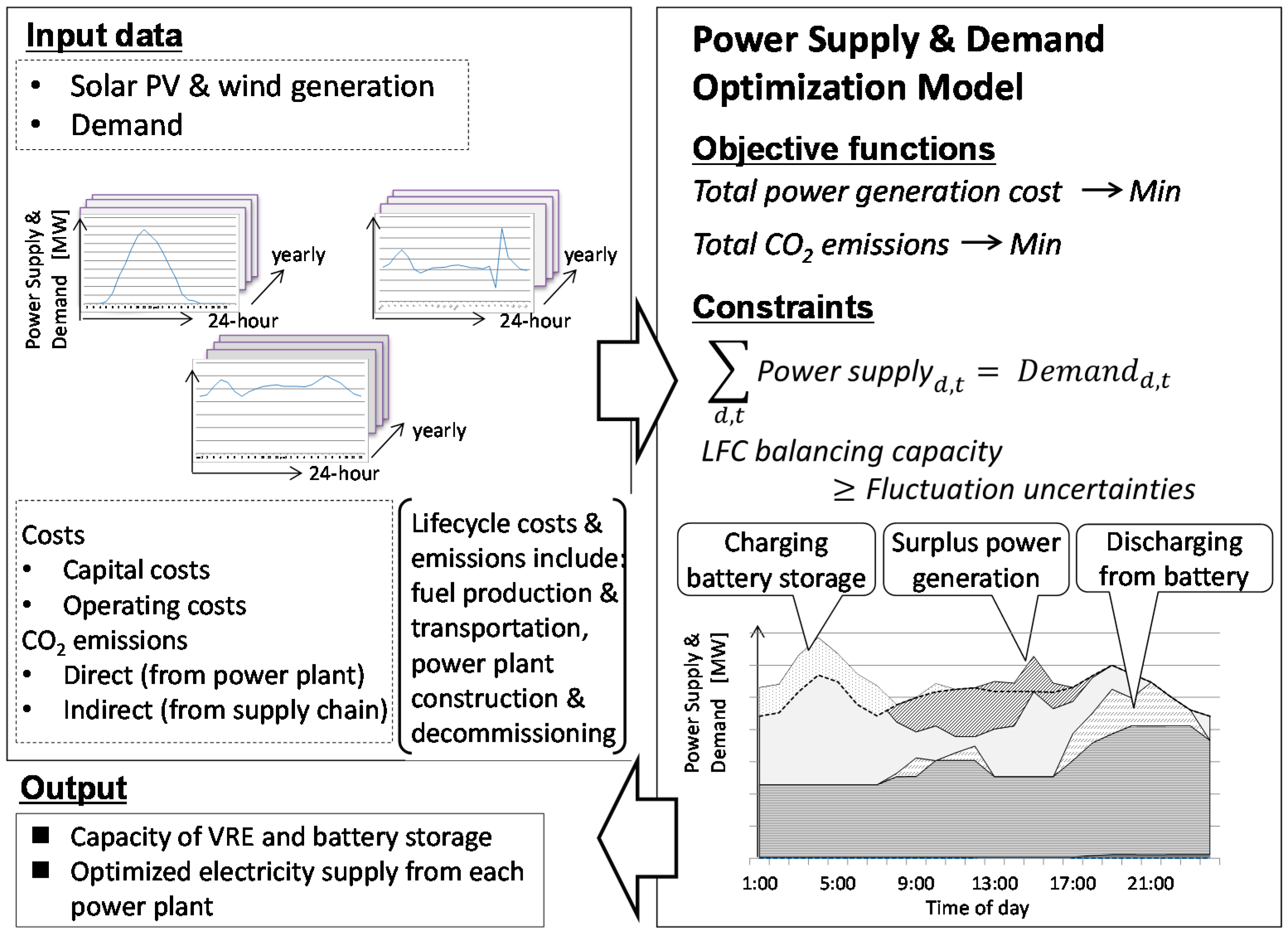
2.1. Overview of the Model

Figure 1 shows an overview of the power supply and demand optimization model that we developed. It is a linear programming model using the software “What’s Best!” (Lindo System Inc., Chicago, IL, USA), a Microsoft Excel-based add-in program, that calculates the optimal capacity of VRE installation to minimize either the total power generation cost or the total CO2 emissions. The total cost depends on the annualized capital cost, the operation and maintenance cost, and the fuel cost, while the CO2 emissions include direct CO2 emissions from thermal plant and indirect annualized life cycle emissions from sources associated with the manufacture of power generation equipment and related infrastructure. The model operates under various constraints to balance electricity demand and supply on an hourly basis, as described below.
Several control options are used to stabilize the grid depending on the timeframe over which variations in supply occur. When the need for control extends over 20 min, an economic dispatch control tool operates to adapt the system to minimize the fuel cost. For variations that occur for less than 20 min but more than a few minutes, load frequency control (LFC) can effectively mitigate the fluctuations in VRE supply. When the range of the fluctuation cycle is less than a few minutes, governor-free control of the thermal plant is invoked to stabilize the grid. Although the model balances supply and demand on an hourly basis, the potential for LFC balancing (by thermal plant and battery storage) of VRE within each hourly period is also considered. The model does not consider balancing by governor-free control.

2.2. Model Configuration

The model’s objective is to minimize the total annual cost of power generation (Equation (1)) or total annual CO2 emissions (Equation (2)).
T o t a l   p o w e r   g e n e r a t i o n   c o s t = i K C o s t i × C a p i + d t C o s t f u e l × E t h e r m a l , d , t + C o s t b a t t e r y × C a p b a t t e r y
T o t a l   C O 2   e m i s s i o n s = i i C O 2 i × C a p i + d t d C O 2 × E t h e r m a l , d , t + C O 2 b a t t e r y × C a p b a t t e r y
In Equation (1), i is the type of power plant (thermal, hydro, wind, or solar PV), K C o s t i [Yen/kW] is the annualized capital cost of power plant i , C a p i [kW] is the capacity of power plant i , C o s t f u e l [Yen/kWh] is the cost of fuel used at the thermal power plant, E t h e r m a l , d , t [kWh] is the amount of electricity generated at the thermal power plant at time t of day d , C o s t b a t t e r y [Yen/kWh] is the annualized cost of battery storage, and C a p b a t t e r y [kWh] is the capacity of battery storage. In addition, in Equation (2) i C O 2 i [t-CO2/kW] is the annualized indirect emissions of CO2 from the power plant i , d C O 2 [t-CO2/kWh] represents the direct emissions of CO2 from fuel combustion in the thermal power plant, and C O 2 b a t t e r y [t-CO2/kWh] is the annualized emissions of CO2 from the battery storage manufacturing process.
The two objective functions are subject to the following constraints.
  • Balancing power supply and demand:
Equation (3) describes how the model balances demand across the grid with the various supply options.
i E i , d , t + D i s d , t C h a d , t = D e m a n d d , t
where E i , d , t [kWh] is the electricity generated from power plant i at time t of day d , D i s d , t [kWh] is the amount of electricity discharged to the grid from battery storage, C h a d , t [kWh] is the amount of electricity sent from the grid to battery storage, and D e m a n d d , t [kWh] is the aggregate electricity demand.
As described in Equation (4), the amount of electricity generated from power plant i is limited by the capacity of that plant. For the thermal power plant, the amount of electricity generated in an hour must be greater than or equal to the hourly output produced at the plant’s minimum operating level, P t h e r m a l , m i n [kW], as shown in Equation (5).
0   E i , d , t C a p i
P t h e r m a l , m i n     E t h e r m a l , d , t
  • Constraints on battery storage
The model assumes storage is provided by a sodium-sulfur battery. Equations (6)–(12) describe the incumbent constraints.
S d ,   t + 1 =   S d , t +   C h a d , t × ε c h a     D i s d , t ε d i s
0     S d , t     C a p b a t t e r y
S 1 , 1 = C a p b a t t e r y   × S O C i n i t
C a p b a t t e r y   =   m s t o r a g e × P b a t t e r y
0     C h a d , t     P b a t t e r y
0     D i s d , t   P b a t t e r y
0     D i s d , t   S d ,   t 1 ×   ε d i s
where S d , t [kWh] is the amount of electricity stored in battery at time t of day d , ε c h a and ε d i s represent the battery’s cycle efficiency for charging and discharging, respectively, S O C i n i t is the battery’s initial state of charge, m s t o r a g e [kWh/kW] is the ratio of the energy storage capacity to the rated output of the battery, which is given by P b a t t e r y [kW].
  • VRE constraints
To balance the grid when supply is greater than demand, some VRE sources may be curtailed, as described in Equation (13). Equation (14) shows that the installed capacity of VRE, C a p V R E [kW], must also be greater than a minimum capacity value, C a p m i n , V R E [kW].
E V R E , d , t = E V R E , d , t ' C u r V R E , d , t
C a p m i n , V R E C a p V R E
where E V R E , d , t [kWh] is the VRE supplied at time t of day d , E V R E , d , t ' [kWh] is the estimated VRE generation, and C u r V R E , d , t [kWh] is the amount of VRE curtailment.
  • LFC constraints
LFC is important to maintain the frequency of the power grid so that concerns to the LFC issues have been addressed in various power system models and control techniques/strategies [20]. In this study, the constraints on LFC expressed in Equations (15)–(22) were taken from the literature [21,22] that is used by Japanese electric power companies to estimate the potential capacity of wind power that can be connected to the power grid. The balanced equation, which assumes that the fluctuations caused by VRE output and demand uncertainties can be absorbed by LFC balancing capacity, is algebraically expressed as Equation (15). Rearranging then allows the direct calculation of the LFC balancing capacity in Equation (16).
k E L F C k 2 + V r e s , d , t 2 V d e m a n d , d , t 2 + l ( U l , d , t 2 )
k E L F C k V d e m a n d , d , t 2 + l ( U l , d , t 2 ) V r e s , d , t 2
E L F C t h e r m a l = C a p t h e r m a l × α t h e r m a l
E L F C b a t t e r y = P b a t t e r y × α b a t t e r y
V d e m a n d , d , t = β d e m a n d × D e m a n d d , t
U w i n d , d , t = β w i n d × C a p w i n d ×   E w i n d ,   d , t E w i n d , d , t '
U P V ,   d , t = β P V × E P V , d , t ' ×   E P V ,   d , t E P V , d , t '
V r e s , d , t = γ r e s × D e m a n d d , t
where k represents the type of LFC balancing capacity (thermal power plant or battery storage), E L F C k [kWh] is the amount of electricity provided from the LFC balancing capacity of type k , V d e m a n d , d , t [kWh] is the variability in demand (from the forecast value) at time t of day d , l represents the type of VRE (wind power or solar PV), U l , d , t [kWh] is the variability in supply of VRE l (from the forecast value), V r e s , d , t [kWh] is the residual variability that cannot be absorbed by LFC, α t h e r m a l and α b a t t e r y represent, respectively, the fraction of the capacity of the thermal power plant and battery storage that is available to provide LFC balancing capacity, β d e m a n d is a coefficient that represents the fraction of demand that varies, β w i n d and β P V represent the variation in supply for wind power and solar PV respectively, and γ r e s is a coefficient that represents the fraction of demand that cannot be met by LFC.
Approximating Equation (16) in a linear form (the development of which is shown in Equations (23)–(28)) then permits evaluation of the amount of VRE curtailment [22].
k E L F C k L b a s e , d , t l ( L b a s e , d , t L l , d , t ) × ( 1 E l , d , t E l , d , t ' )
L b a s e , d , t = V d e m a n d , d , t 2 + l ( U l , d , t ' 2 ) V r e s , d , t 2
L w i n d , d , t = V d e m a n d , d , t 2 + U P V , d , t ' 2 V r e s , d , t 2
L P V , d , t = V d e m a n d , d , t 2 + U w i n d , d , t ' 2 V r e s , d , t 2
U w i n d , d , t ' =   β w i n d ×   C a p w i n d
U P V , d , t ' = β P V   ×   E P V , d , t '

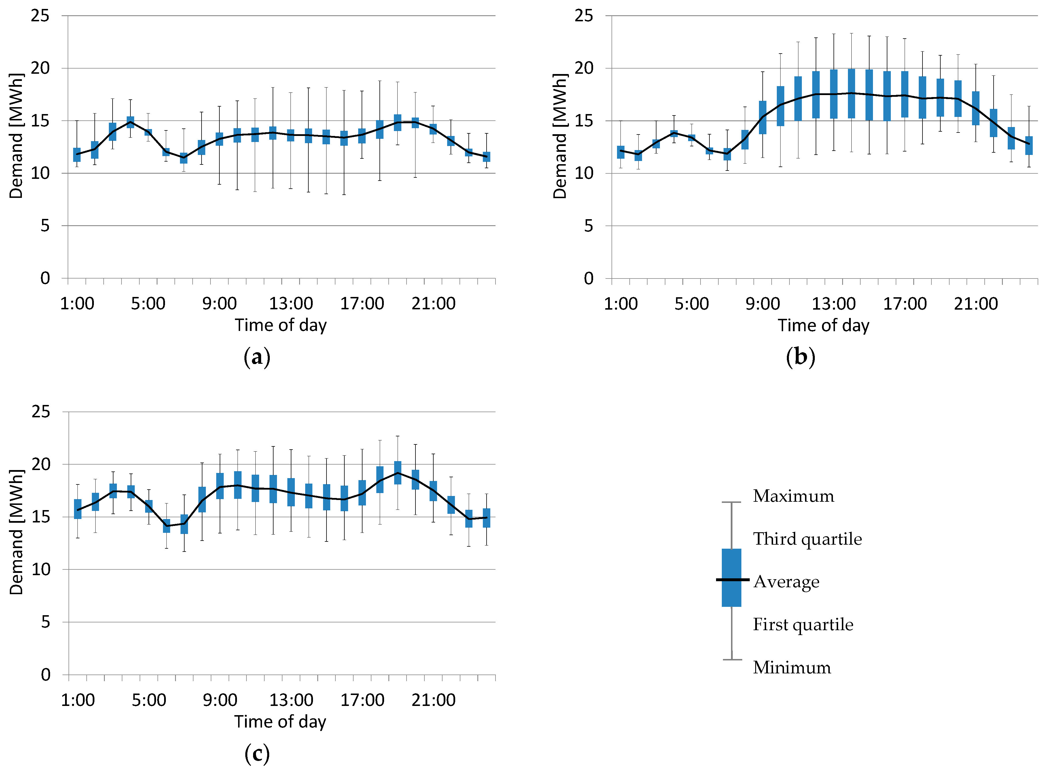
2.3. Case Study Site and Its Electricity Supply and Demand Data

The case study site was a remote island located in western Japan. As of 2011, the island had a population of 20,000, which was distributed among 10,000 households. Tertiary industries employed the largest portion of the population, and 80% of the island was covered by forest. Three types of power plant provided electricity to the island’s grid; 32.7 MW of diesel thermal plant fueled by heavy fuel oil, 0.3 MW of hydropower, and 1.8 MW of wind power. A further 0.4 MW of residential solar PV was installed across some of the island’s households.
Electricity supply data for the three power plants and an estimate of the electricity generated by solar PV (see Section 2.4.2 for method) were summed to estimate aggregate demand for financial year (FY) 2011 (April 2011–March 2012).
Figure 2 shows the distribution of diurnal electricity demand for three stages in the year (midseason: April–June and October–November; summer: July–September; and winter: December–March). Total demand during FY 2011 was 131 GWh. The minimum hourly demand of approximately 8 MWh was observed at 16:00 in the midseason while the maximum value of approximately 23 MWh was observed at 14:00 in summer. The daily variation in hourly demand was largest in the summer.

2.4. VRE Power Generation Estimates
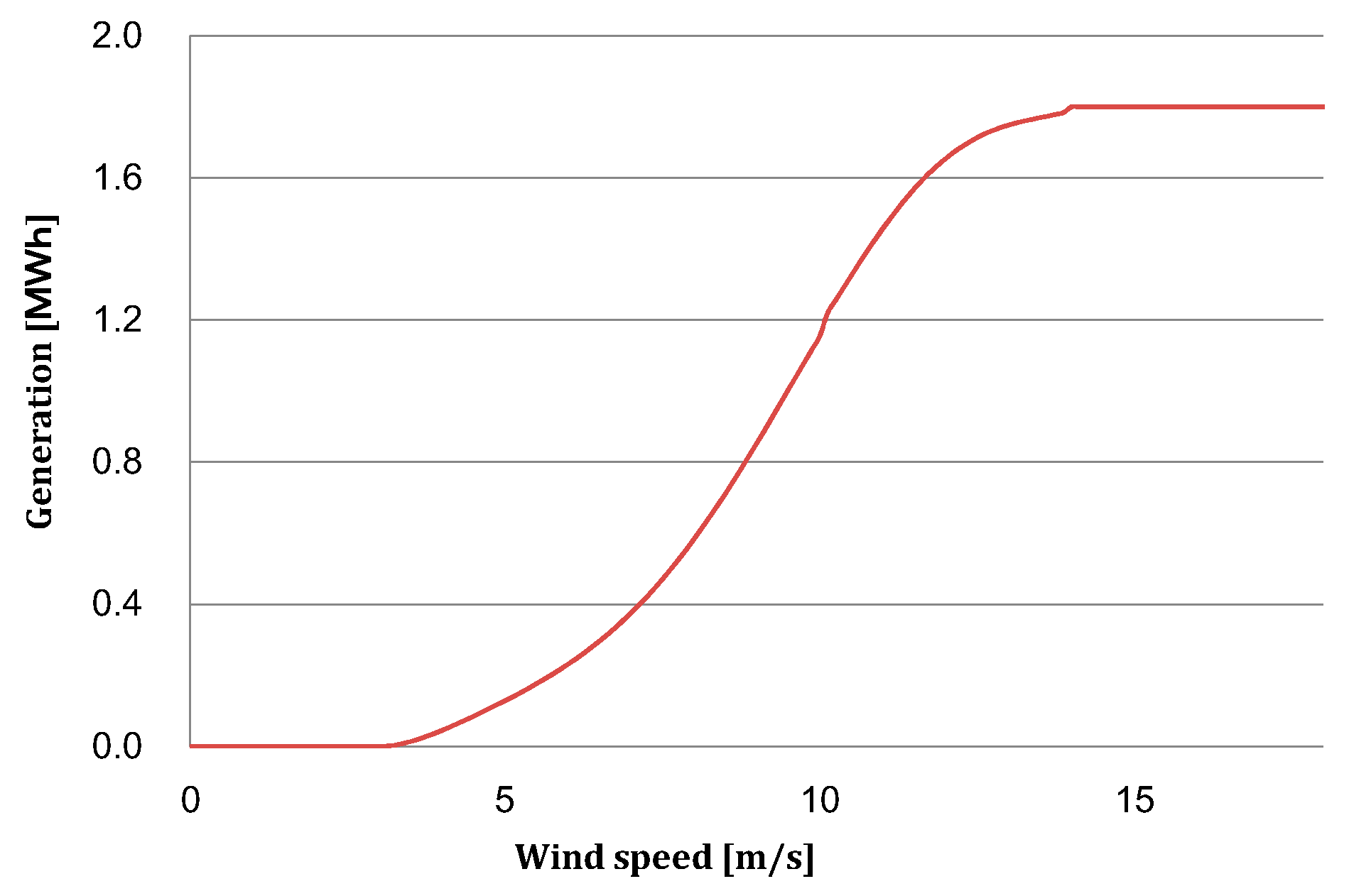
2.4.1. Wind Power

The amount of wind power supplied to the grid does not necessarily reflect the total wind powered generation because it cannot account for any wind power that was curtailed. We therefore employ the following schema to estimate the total electricity generated from wind power.
The hourly average wind speed V [m/s] at an altitude of Z [m] can be calculated using Equation (29) [23] and a reference wind speed value, V1 [m/s], taken from a point in the same location at a height of Z1 [m] of the Japanese Automated Meteorological Data Acquisition System (AMeDAS) [24]. The value of n in Equation (29) was set to 3.5, as the literature suggests [23]. The power curve of the turbine can then be calculated (Equation (30)). Figure 3 shows the power curve of a 500 kW wind turbine, which was assumed to be representative for the case study site.
V d , t = V 1   d , t ( Z Z 1 ) 1 n
E w i n d , d , t ' = F ( V d , t )

2.4.2. Solar PV

With no primary data available for the case study site, the hourly solar PV generation was calculated using Equation (31).
E P V , d , t ' = S R i n / X × C a p P V × ( 1 a ) × ( 1 b ) × ( 1 c )
where S R i n [kWh/m2] is the solar irradiance of an inclined surface, X [kW/m2] is the standard solar irradiance, a is the temperature loss coefficient (set to 15% for March–May and September–November, 20% for June–August, and 10% for December–February), and b and c are losses caused by the inverter and within the solar PV system, respectively, both of which were set to 5% in agreement with assumptions made by the Japanese industry. The solar irradiance of an inclined surface is the sum of direct, reflected, and diffuse solar irradiance [25]. These terms were calculated using the variables summarized in Table A1 (Appendix A) [26,27]. The number of sunshine hours at the case study site in FY 2011 were sourced from AMeDAS) [24]. The inclination and azimuth angles of the solar PV cell were set to 30° and 22.5°, respectively.

2.5. Model Parameters

Table 1 details the parameters used to calculate the total power generation cost and total CO2 emissions at the case study site. Capital cost represents the sum of the annualized construction cost, property tax, and decommissioning cost. Operating cost is the sum of annual labor, maintenance, and administrative costs. The fuel costs for the diesel thermal plant were calculated using fuel charges [28], the price of heavy fuel oil [29], the plant’s thermal efficiency [30], and the fuel’s calorific value [31]. Indirect emissions from the power plant included annualized lifecycle emissions accruing from the construction and manufacturing process and those produced by the fuel supply chain. Table 2 presents the costs and CO2 emissions data used for battery storage, with other miscellaneous model parameters shown in Table 3.

2.6. Simulation Cases Settings

The base case represents the current situation (32.7 MW of diesel thermal plant, 0.3 MW of hydro power, 1.8 MW of wind power, and 0.4 MW of solar PV, no battery storage). Cases 2 and 3 simulate the optimal capacity of VRE to install to meet current electricity demand without (Case 2) and with (Case 3) battery storage.

3. Results and Discussion

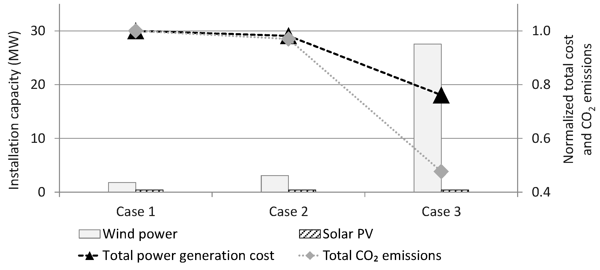
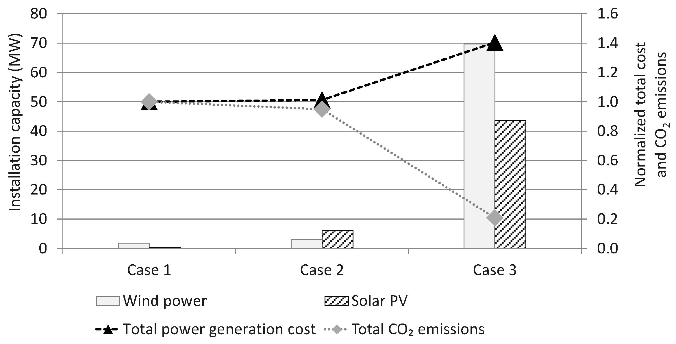
3.1. Total Power Generation Cost Minimization

Figure 4 shows the installed capacity of VRE and battery storage for the various cases when minimizing the total power generation cost. The total cost of generation and the total associated CO2 emissions are also shown, normalized to those from the base case (Case 1: 3328 million Yen and 98,278 t-CO2, respectively). In Case 2 the optimized capacity of wind power was 3 MW (1.7 times greater than that in the base case). The total generation cost and total CO2 emissions were found to be 98% and 97% of those calculated in Case 1, respectively. Both decreases were attributed to a decrease in fuel usage at the diesel thermal power plant. Installing 73 MWh of battery storage (Case 3) had a significant impact on the VRE capacity. Wind power capacity increased to 28 MW (15.8 times that of Case 1), while the total power generation cost and total CO2 emissions were found to be 76% and 48% of those calculated in Case 1, respectively. In both Cases 2 and 3, the installed capacity of solar PV did not increase because it was more economic to install extra wind-powered capacity instead.

3.2. Example Generation Mix
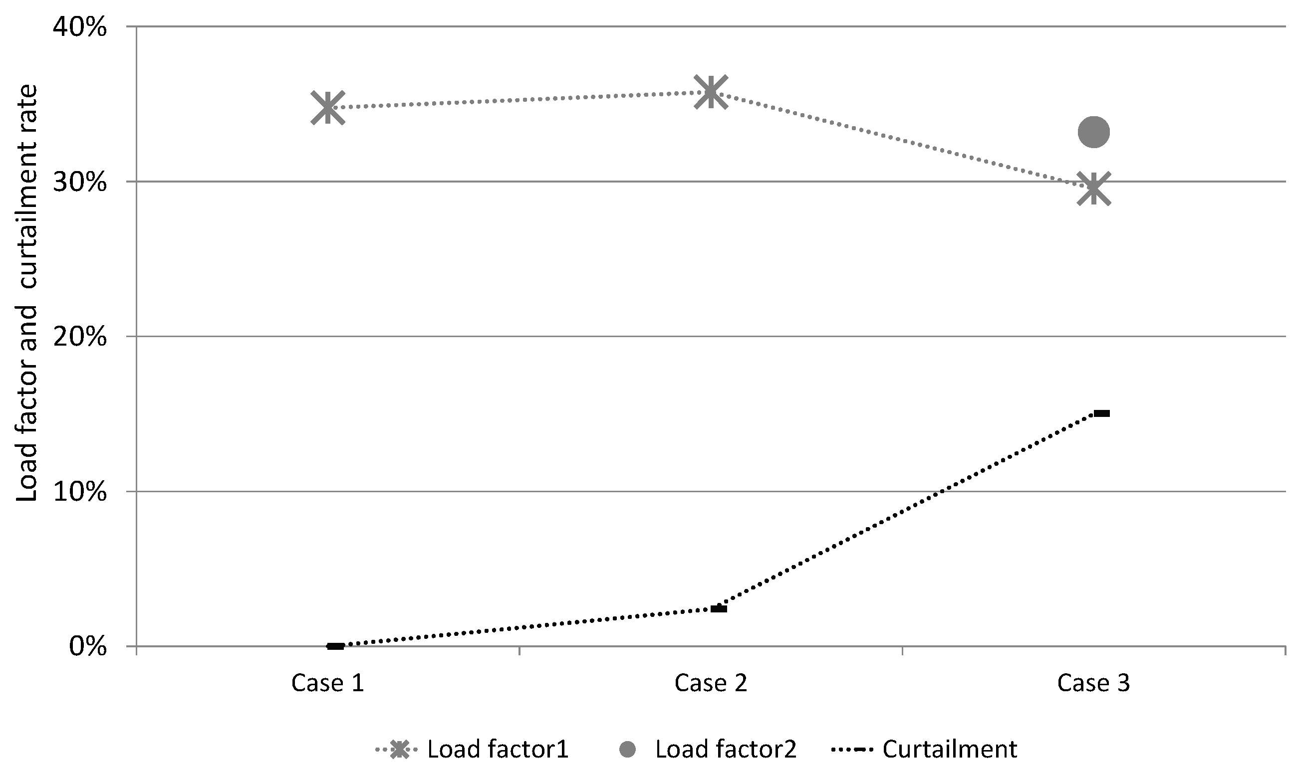
The calculated hourly generation mixes for the period 1–20 August 2011 for the three cases are shown in Figure 5. Diesel thermal power is the main source of electricity in Case 1 (Figure 5a) and no VRE curtailment was observed. In Case 2 (Figure 5b), the 1.7 increase in installed wind power capacity resulted in VRE curtailment because of the LFC constraint (see Equation (23)). In Case 3 (Figure 5c), VRE capacity significantly substituted generation from diesel thermal power on several days. Frequent charging and discharging of battery storage failed to entirely prevent VRE curtailment, and low VRE generation during some hours meant that, at times, diesel thermal power was still the main electricity source. This suggests that conventional thermal power can play an important role in ensuring a stable electricity supply.

3.3. Load Factor

The introduction of battery storage was expected to increase the load factor of VRE capacity as batteries allow excess electricity generated above the level demanded to be stored instead of curtailed. To investigate this, the load factor of VRE capacity was evaluated for each of the simulation cases. The load factor (LF1) calculated in Equation (32) represents the ratio of the annual electricity supply from VREs to the total theoretical electricity supply from the installed capacity. The alternative load factor described in Equation (33) (LF2) includes an appreciation of indirect VRE generation via battery storage. Please note that FY 2011 was a leap year.
L F 1 = l d t E l , d , t / l C a p l × 24 × 366
L F 2 = ( l d t E l , d , t " + d t D i s d , t ) / l C a p l × 24 × 366
where E l , d , t " is the direct electricity supply from VRE l . Figure 6 presents the load factor values for the three cases. From Case 1 to Case 2, LF1 increased by 1 percentage point, even though VRE curtailment increased from zero to almost 2%. This was alongside the decrease in cost observed above. In Case 3, which had a significantly higher installed wind power capacity alongside battery storage and an even lower total power cost, the load factor was the lowest of the three cases because of an increase in VRE curtailment. Even when accounting for secondary capacity via the battery storage, the load factor in Case 3 did not reach the levels observed in the other cases. Thus, at a grid-optimization level, the addition of battery storage does not necessarily lead to increased load factors if the same optimization also involves adding significant amounts of VRE to the grid.

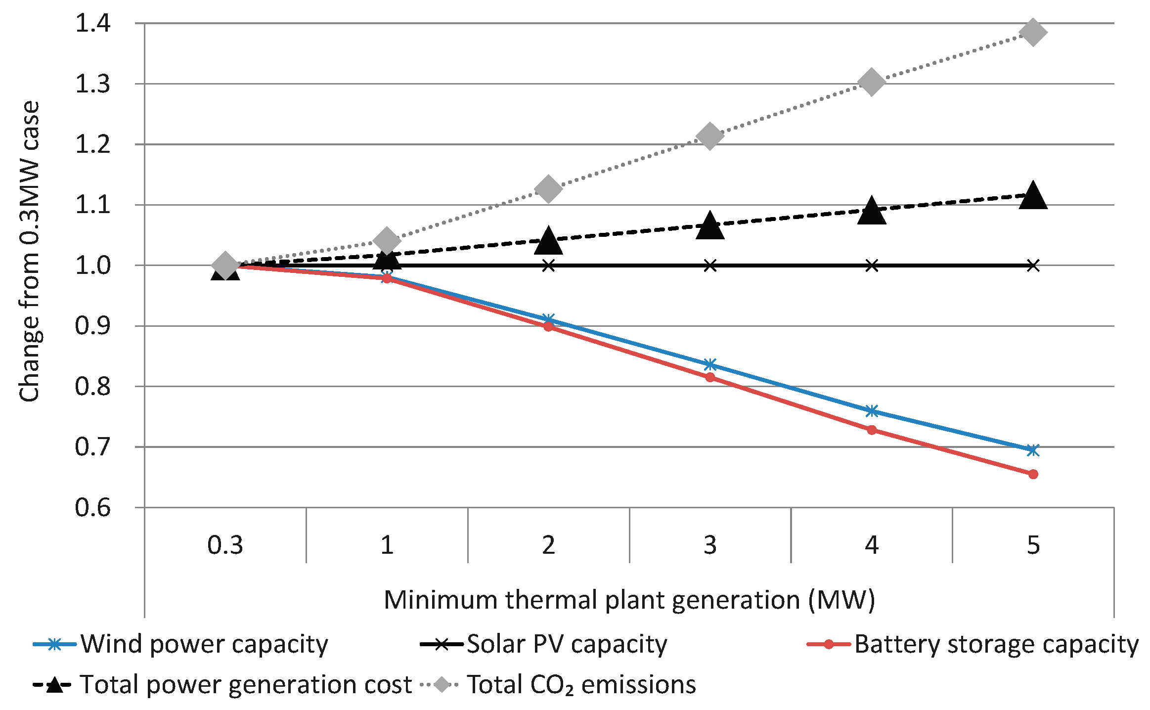
3.4. Sensitivity to Minimum Thermal Plant Generation

As described in Equation (5) and Table 3, the minimum output of the thermal power plant was set to 0.3 MW. However, because this parameter affects the usage of VRE on the grid and therefore the optimal installed VRE capacity, we decided to conduct a sensitivity analysis on this parameter. The lowest hourly electricity supply from the thermal power in Case 2 was 6 MWh, 20 times greater than the minimum threshold. Thus, the sensitivity study was only carried out for Case 3.
Figure 7 shows how the installed VRE capacity, required battery storage, total cost, and total CO2 emissions varied with changes to the minimum thermal plant output. As the minimum output of thermal power was increased, the amount of VRE-generated electricity decreased. The installed VRE and battery capacity also fell from 28 MW of wind power and 73 MWh of battery storage with a minimum thermal plant output of 0.3 MW to 19 MW of wind power and 48 MWh of battery storage when the minimum thermal plant output was increased to 5 MW. As these capacity values decreased, the total power generation cost and the total emissions of CO2 increased by 10% and 40%, respectively. These high sensitivities suggest that significant effort should be made to use accurate values for minimum plant load when conducting this type of modelling.

3.5. Minimizing Total CO2 Emissions

Figure 8 shows the case study optimization results to minimize total CO2 emissions. The installation of both VRE technologies increased compared with the base case, with the installed capacity of solar PV much higher than in the cost-minimization approaches (Figure 4), reaching, for example, 6 MW for Case 2 (compared with 0.4 MW for Case 2 in the cost-optimization approach). Adding VRE capacity in Case 2 resulted in a 5% decrease in CO2 emissions, because less power was generated by the diesel thermal plant, and a 1% increase in total cost, as the decrease in operating costs for the diesel thermal plant was offset by increased VRE capital costs. For Case 3, the emissions-minimization approach resulted in the installed capacity of wind power expanding to 70 MW (28 MW in cost-minimization approach) and that of solar PV reaching 44 MW (0.4 MW in cost-minimization approach). The capital costs associated with this increase in VRE capacity and battery storage led to a 40% increase in the total cost over that of the base case, though this approach produced just 21% of the base case’s CO2 emissions as the amount of energy sourced from thermal power decreased significantly.

4. Conclusions

A model that optimizes power supply to meet demand was developed to evaluate the potential for installing VRE capacity by considering the hourly grid balance and LFC constraints. The model was applied to a case study of a remote Japanese island that is dependent on diesel thermal power generation and was optimized to minimize either the total power costs or the total power-related CO2 emissions.
Simulations suggest that the VRE capacity could be increased from the baseline values of 1.8 MW of wind power and 0.4 MW of solar PV. The degree to which it was economic to install VRE depended on whether battery storage was available. The cost-optimization model calculated that the capacity of wind power should be expanded by a factor of 1.7 if storage was not available (Case 2), but by a factor of 15.8 if 73 MWh of battery storage was also installed (Case 3). This resulted in total costs that were 2% and 24% lower than the baseline and decreases in total CO2 emissions of 3% and 52%, for Cases 2 and 3, respectively. The capacity of solar PV did not change in the cost-optimization model because wind power was always cheaper for the model to procure. The main reason for the changes that resulted was attributed to decreased fuel usage for the diesel thermal power plant. Optimizing the scenarios to minimize the total CO2 emissions showed that the installation of 307 MWh of battery storage could permit CO2 emissions that were 21% of those in the base case, though the total cost would increase by 40%. A sensitivity analysis showed that when battery storage was available, the results were notably impacted by the thermal plant’s minimum output threshold.
We hope that the findings in this work will be useful to governments interested in implementing climate change mitigation technologies in isolated power grids. In particular, this work may help to illustrate the potential of developing VRE in such grids while maintaining stable supply. However, we urge interested parties to also take account of exogenous factors not modeled here, such as the impact of population change on energy demand, to support decision makers in the further development of power grids.

Author Contributions

Mai Inoue conducted the analysis and wrote the paper under the guidance of Yutaka Genchi and Yuki Kudoh All authors checked and approved the final draft.

Conflicts of Interest

The authors declare no conflict of interest.

Appendix A

Table A1. Decomposition of solar irradiation on an inclined surface.
IrradianceVariables UsedCalculation Notes
Direct normal irradiance on inclined surface1. Direct normal irradianceCalculated from global horizontal irradiance and the diffuse horizontal irradiance.
2. Angle of incidence angle for direct irradiance to solar PV cell surfaceCalculated using the solar PV cell’s inclination and azimuth angles.
3. Solar altitudeCalculated using the declination and hour angle of the sun, which are determined astronomically, and the latitude of the site.
Reflected solar irradiance on inclined surface4. Global horizontal irradianceCalculated using the extraterrestrial irradiance—which is determined from the solar constant, solar altitude and geocentric solar distance—and the ratio of sunshine hours and hours of daylight.
5. Inclination angle of solar PV cell
Diffuse solar irradiance on inclined surface6. Diffuse solar irradianceCalculated using the ratio of global horizontal irradiance and extraterrestrial irradiance.
7. Inclination angles of solar PV cell

References

  1. Lund, H. Renewable energy strategies for sustainable development. Energy 2007, 32, 912–919. [Google Scholar] [CrossRef]
  2. Evans, A.; Strezov, V.; Evans, T.J. Assessment of sustainability indicators for renewable energy technologies. Renew. Sustain. Energy Rev. 2009, 13, 1082–1088. [Google Scholar] [CrossRef]
  3. Jaramillo-Nieves, L.; del Río, P. Contribution of Renewable Energy Sources to the Sustainable Development of Islands: An Overview of the Literature and a Research Agenda. Sustainability 2010, 2, 783–811. [Google Scholar] [CrossRef]
  4. Dincer, I. Renewable energy and sustainable development: A crucial review. Renew. Sustain. Energy Rev. 2000, 4, 157–175. [Google Scholar] [CrossRef]
  5. International Energy Agency (IEA). Medium-Term Renewable Energy Market Report 2015; OECD/IEA: Paris, France, 2015. [Google Scholar]
  6. United Nations Framework Convention on Climate Change (UNFCCC). Report of the Conference of the Parties on Its Twenty-First Session; UNFCCC: Berlin, Germany, 2015. [Google Scholar]
  7. Cochran, J.; Bird, L.; Heeter, J.; Arent, D.J. Integrating Variable Renewable Energy in Electric Power Markets: Best Practices from International Experience, Summary for Policymakers; NREL (National Renewable Energy Laboratory, U.S. Department of Energy): Golden, CO, USA, 2012.
  8. Agency for Natural Resources and Energy; Japan Ministry of Economy, Trade and Industry (METI). Feed-In Tariff Scheme in Japan; METI: Tokyo, Japan, 2012.
  9. Nikkei, B.P. Kyushu Electric Announces Output Restriction Records. Available online: http://techon.nikkeibp.co.jp/atclen/news_en/15mk/051000562/?ST=msbe (accessed on 20 July 2016).
  10. Baños, R.; Manzano-Agugliaro, F.; Montoya, F.G.; Gil, C.; Alcayde, A.; Gómez, J. Optimization methods applied to renewable and sustainable energy: A review. Renew. Sustain. Energy Rev. 2011, 15, 1753–1766. [Google Scholar] [CrossRef]
  11. Connolly, D.; Lund, H.; Mathiesen, B.V.; Leahy, M. A review of computer tools for analysing the integration of renewable energy into various energy systems. Appl. Energy 2010, 87, 1059–1082. [Google Scholar] [CrossRef]
  12. Luderer, G.; Krey, V.; Calvin, K.; Merrick, J.; Mima, S.; Pietzcker, R.; van Vliet, J.; Wada, K. The role of renewable energy in climate stabilization: Results from the EMF27 scenarios. Clim. Chang. 2014, 123, 427–441. [Google Scholar] [CrossRef] [Green Version]
  13. Shiraki, H.; Ashina, S.; Kameyama, Y.; Hashimoto, S.; Fujita, T. Analysis of Optimal Locations for Power Stations and Their Impact on Industrial Symbiosis Planning under Transition toward Low-carbon Power Sector in Japan. J. Clean. Prod. 2016, 114, 81–94. [Google Scholar] [CrossRef]
  14. Komiyama, R.; Fujii, Y. Assessment of massive integration of photovoltaic system considering rechargeable battery in Japan with high time-resolution optimal power generation mix model. Energy Policy 2014, 66, 73–89. [Google Scholar] [CrossRef]
  15. Komiyama, R.; Otsuki, T.; Fujii, Y. Energy modeling and analysis for optimal grid integration of large-scale variable renewables using hydrogen storage in Japan. Energy 2015, 81, 537–555. [Google Scholar] [CrossRef]
  16. Ogimoto, K.; Kataoka, K.; Ikegami, T.; Nonaka, S.; Azuma, H.; Fukutome, S. Demand–Supply Balancing Capability Analysis for a Future Power System. Electr. Eng. Jpn. 2014, 186, 21–30. [Google Scholar] [CrossRef]
  17. Yoo, K.; Park, E.; Kim, H.; Ohm, J.Y.; Yang, T.; Kim, K.J.; Chang, H.J.; del Pobil, A.P. Optimized Renewable and Sustainable Electricity Generation Systems for Ulleungdo Island in South Korea. Sustainability 2014, 6, 7883–7893. [Google Scholar] [CrossRef]
  18. Senjyu, T.; Hayashi, D.; Yona, A.; Urasaki, N.; Funabashi, T. Optimal configuration of power generating systems in isolated island with renewable energy. Renew. Energy 2007, 32, 1917–1933. [Google Scholar] [CrossRef]
  19. Duić, N.; Carvalho, M.D.G. Increasing renewable energy sources in island energy supply: Case study Porto Santo. Renew. Sustain. Energy Rev. 2004, 8, 383–399. [Google Scholar] [CrossRef]
  20. Pandey, S.K.; Mohanty, S.R.; Kishor, N. A literature survey on load–frequency control for conventional and distribution generation power systems. Renew. Sustain. Energy Rev. 2013, 25, 318–334. [Google Scholar] [CrossRef]
  21. Kuramoto, M.; Nagata, M.; Inoue, T. A Modified Algebraic Method to Evaluate Required Capacity for Frequency Control under a Large Penetration of Solar PV Generations; Research Report 2011, R10005; CRIEPI (Central Research Institute of Electric Power Industry): Tokyo, Japan, 2011. (In Japanese) [Google Scholar]
  22. Yamamoto, H.; Bando, S.; Sugiyama, M. Development of a Power Generation Mix Model Considering Multi Modes of Operation of Thermal Power Fleets and Supply-Demand Adjustability; Research Report 2014, Y12030; CRIEPI (Central Research Institute of Electric Power Industry): Tokyo, Japan, 2014. (In Japanese) [Google Scholar]
  23. New Energy and Industrial Technology Development Organization (NEDO). Guidebook on Wind Power Introduction; NEDO: Tokyo, Japan, 2008. (In Japanese)
  24. Japan Meteorological Agency, Japan (JMA). Automated Meteorological Data Acquisition System (AMeDAS). Available online: http://www.data.jma.go.jp/obd/stats/etrn/index.php (accessed on 20 July 2016). (In Japanese)
  25. New Energy and Industrial Technology Development Organization (NEDO). Reference of NEDO Standard Meteorological database. Japan Weather Association. Available online: http://www.nedo.go.jp/content/100778067.pdf (accessed on 20 July 2016). (In Japanese)
  26. Erbs, D.G.; Klein, S.A.; Duffie, J.A. Estimation of the Diffuse Radiation Fraction for Hourly, Daily and Monthly Average Global Radiation. Sol. Energy 1982, 28, 293–302. [Google Scholar] [CrossRef]
  27. Masaki, Y.; Kuwagata, T.; Ishigooka, Y. Precise estimation of hourly global solar radiation for micrometeorological analysis by using data classification and hourly sunshine. Theor. Appl. Climatol. 2010, 100, 283–297. [Google Scholar] [CrossRef]
  28. Cost Verification Committee. Report of the Cost Verification Committee 2011; Cabinet Office, Government of Japan: Tokyo, Japan, 2011. (In Japanese)
  29. Agency for Natural Resources and Energy; Ministry of Economy, Trade and Industry (METI). Price Survey of Petroleum Products 2011; METI: Tokyo, Japan, 2011. (In Japanese)
  30. Imamura, E.; Nagano, K. Evaluation of Life Cycle CO2 Emissions of Power Generation Technologies—Update for State-of-the-Art Plants; Research Report 2010, Y09027; CRIEPI (Central Research Institute of Electric Power Industry): Tokyo, Japan, 2010. (In Japanese) [Google Scholar]
  31. Japan Automobile Research Institute (JARI); Special Committee of Synthesis Study on Efficiency. The Results about Efficiency from Synthesis Study; JHFC Japan Hydrogen & Fuel Cell Demonstration Project; Japan Automobile Research Institute (JARI): Tsukuba, Japan, 2006. (In Japanese) [Google Scholar]
  32. World Bank. Official Exchange Rate (LCU per USS, Period Average). Available online: http://data.worldbank.org/indicator/PA.NUS.FCRF?locations=JP (accessed on 12 August 2016).
  33. Ministry of Economy, Trading and Industry (METI). Strategy of Battery 2012; Project Team for Strategy of Battery; METI: Tokyo, Japan, 2012. (In Japanese)
  34. Sullivan, J.; Gaines, L. A Review of Battery Life-Cycle Analysis: State of Knowledge and Critical Needs; Argonne National Laboratory Report 2010, ANL/ESD/10-7; Argonne National Laboratory: Argonne, IL, USA, 2010.
  35. Komiyama, R.; Shibata, S.; Nakamura, Y.; Fujii, Y. Analysis of Possible Introduction of PV Systems Considering Output Power Fluctuations and Battery Technology, Employing an Optimal Power Generation Mix Model. Electr. Eng. Jpn. 2013, 182, 9–19. [Google Scholar] [CrossRef]
Figure 1. Schematic overview of the model.
Sustainability 09 00119 g001
Figure 2. Diurnal electricity demand throughout the year for the remote island grid. (a) Midseason; (b) Summer; (c) Winter.
Sustainability 09 00119 g002
Figure 3. Power curve of a 500 kW wind turbine.
Sustainability 09 00119 g003
Figure 4. Installed VRE capacity (bars) and the associated total power generation cost and total CO2 emissions normalized to the base case (lines) when minimizing total power generation cost.
Sustainability 09 00119 g004
Figure 5. Calculated hourly generation mix for the period 1–20 August 2011 for the three cases, which were optimized to minimize the total power generation cost. (a) Case 1 (Base case); (b) Case 2 (Without battery storage installation); (c) Case 3 (With 73 MWh battery storage installation).
Sustainability 09 00119 g005
Figure 6. Load factors and curtailment rates for the three cases under a least-cost approach.
Sustainability 09 00119 g006
Figure 7. Sensitivity to minimum thermal plant output in Case 3 under a least-cost approach.
Sustainability 09 00119 g007
Figure 8. Installed VRE capacity (bars) and the associated total power generation cost and total CO2 emissions normalized to the base case (lines) when minimizing total CO2 emissions.
Sustainability 09 00119 g008
Table 1. Cost- and emissions-related model parameters for power generation technologies [28,29,30,31]. 1 USD = 121.04 JPY [32].
Diesel Thermal PlantHydro Power PlantWind Power PlantResidential Solar PV System
Reference for cost estimate [28]400 MW oil-fired0.2 MW20 MW onshore4 kW residential
Capital cost [Yen/kW] [28]505426,63314,89623,100
Operation cost [Yen/kW] [28]668174,10013,5668250
Fuel cost [Yen/kWh]23.05 ---
Reference for emissions estimate [30]1000 MW heavy oil10 MW 0.6 MW onshore4 kW residential
Indirect emissions [t-CO2/kW] [30]0.320.040.040.05
Direct emissions [t-CO2/kWh] [30]0.0007n/an/an/a
Table 2. Cost- and emissions-related model parameters for sodium–sulfur battery storage.
Model ParameterValue
Manufacturing cost [Yen/kWh] [33]2667
Emissions from manufacturing stage [t-CO2/kWh] [34]0.008
Table 3. Miscellaneous model parameter settings.
ParameterValue
P t h e r m a l , m i n 0.3 [MW]
ε c h a ,   ε d i s 95%
S O C i n i t 20%
  m s t o r a g e 6 [kWh/kW] [35]
α t h e r m a l 5%
α b a t t e r y 100%
β demand 4%
β reg 1%
β wind 50%
β PV 50%

