Scenario Prediction of Energy Consumption and CO₂ Emissions in China’s Machinery Industry

Abstract

Energy conservation and CO₂ abatement is currently an important development strategy for China. It is significant to analyze how to reduce energy consumption and CO₂ emissions in China’s energy-intensive machinery industry. We not only employ a cointegration method and scenario analysis to predict the future energy demand and CO₂ emissions in China’s machinery industry, but we also use the Monte Carlo simulation to test the validity of the predictions. The results show that energy demand in the industry will respectively reach 678.759 Mtce (million ton coal equivalent) in 2020 and 865.494 Mtce in 2025 under the baseline scenario. Compared with the baseline scenario, the energy savings in 2020 will respectively be 63.654 Mtce and 120.787 Mtce in the medium and advanced scenarios. Furthermore, we forecast the corresponding CO₂ emissions as well as the reduction potential respectively in 2020 and 2025. In order to achieve energy conservation and emissions reduction, the government should increase energy price, levy environmental taxes based on the emissions level of machinery enterprises, promote mergers and acquisitions of enterprises, and expand the scale of enterprises. This paper provides a reference for energy conservation and CO₂ abatement policy in China’s machinery industry.

1. Introduction

The machinery industry is the main body of the manufacturing sector and the pillar industry of the national economy. It provides not only equipment for the industry, agriculture, transportation, defense, etc., but also the material and technical foundation of the national economy. In line with the classification of the industrial structure, the machinery industry is an important part of the secondary industry. With the accelerating industrialization and urbanization processes in China, the industry maintained a rapid growth trend considering output, energy consumption as well as CO₂ emissions. High energy consumption is one of the important attributes of China’s machinery industry. Energy intensity in China is higher than that in developed countries like Japan and Germany. Due to the serious environmental pollution caused by fossil energy consumption, low-carbon development is the key to constraining the use of fossil fuel. This compels the machinery industry to strengthen the innovation and extension of energy-saving technology, promote clean production, and improve energy efficiency.

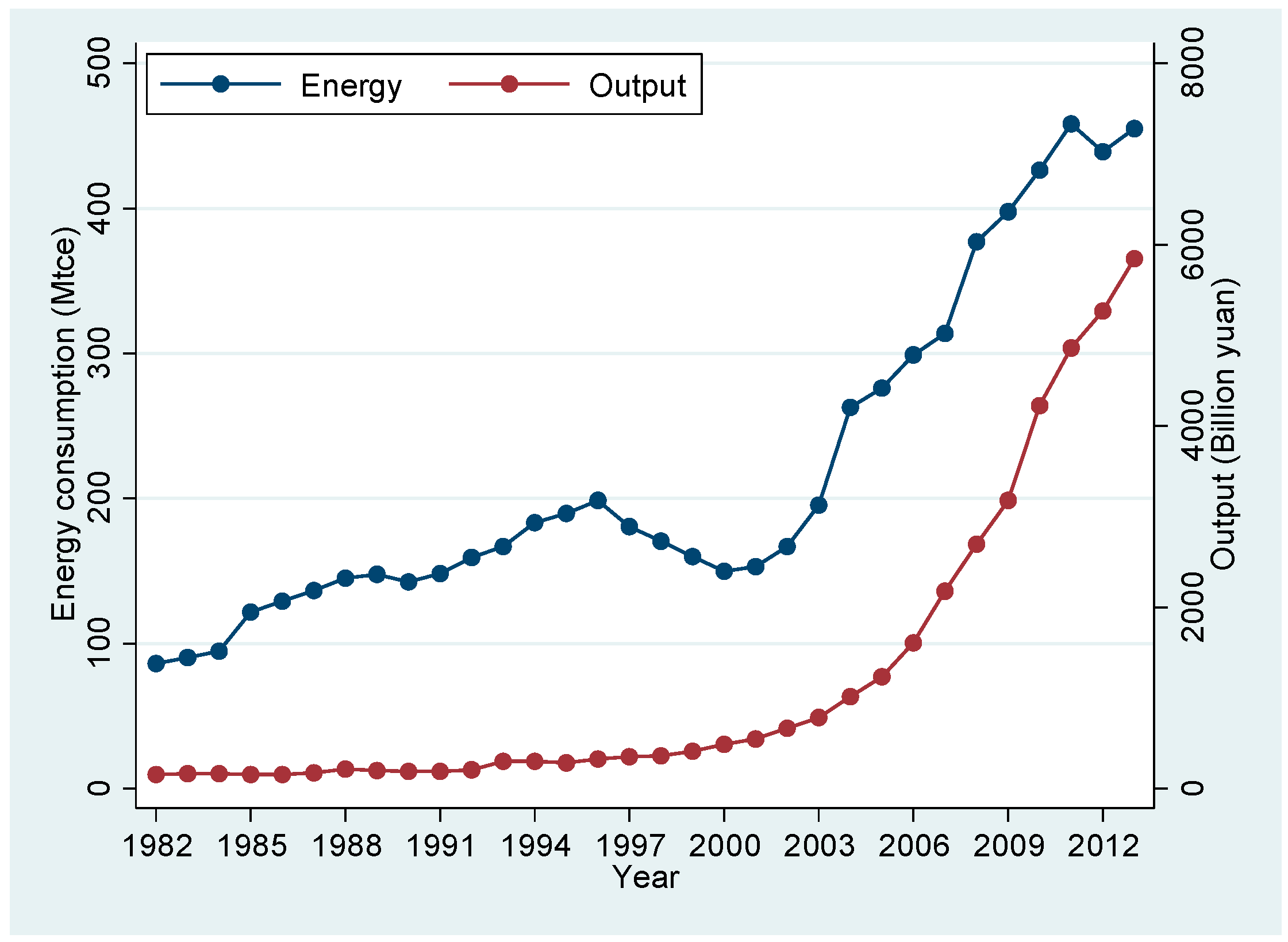
Energy consumption in China’s machinery industry rose from 86.13 Mtce (million ton coal equivalent) in 1982 to 455.17 Mtce in 2013, with an average growth rate of 5.9% [1]. Its output (industrial added value) rose from 152.16 billion yuan in 1982 to 5841.63 billion yuan in 2013, with an average growth rate of 13.2%. As Figure 1 shows, during the period of 1982–2013, the output and energy consumption of the industry showed a general upward trend. The Asian financial crisis of 1997 led to the abrupt decline in energy consumption over the next several years. However, the inventory of mechanical products was still on the rise. Hence, the output did not reduce. Lin and Liu [2] also found a similar phenomenon in the relationship between electricity consumption and economic growth in China.

Increasing energy consumption and environmental pollution as well as CO₂ emissions have caused great concern around the world. China has surpassed the United States as the largest energy consumer in the world. Compared with developed countries, China’s energy structure needs to be optimized and energy efficiency should be improved in China. An extensive economic growth model has facilitated tremendous development in China for decades, but the model has also caused unsustainable energy consumption and greenhouse gas emissions. The adjustment of economic structure is also imperative, as intensive economic growth is the predicted development trend. China is currently in a crucial stage of promoting economic transformation, whereas energy conservation and CO₂ abatement is still an important development strategy. It requires more advanced and energy-efficient machinery equipment, thereby promoting transformation and upgrading of the machinery industry.

Exploring how to reduce energy consumption and CO₂ emissions in China’s machinery industry is necessary. To understand the coordinated development of energy and economy as well as the environment, some scholars have studied relevant factors that profoundly affect energy demand from different perspectives. In this article, we mainly focus on the following four aspects: (1) Which factors affect energy consumption in China’s machinery industry? (2) How much is the energy conservation potential? (3) How much is the CO₂ emissions reduction potential? (4) How can energy conservation and CO₂ abatement be achieved? Solving these problems will be beneficial to the sustainable development of China’s machinery industry, and reduce energy consumption.

We present the research in the following order. Section 2 consists of a brief literature review of works related to China’s machinery industry and its energy consumption. Section 3 introduces the methodology and data sources. In this part, we describe the cointegration method, the Granger test of causality, as well as IRF (impulse response function) and FEVD (forecast-error variance decomposition). Scenario analysis is employed to estimate the potential of energy conservation and CO₂ abatement. In addition, we illustrate relevant data about the explanatory variables correlated with energy consumption. Section 4 is the empirical analysis, using econometric theory and the method outlined in Section 3 to test and process the data. The results of the empirical analysis are presented in this section. In Section 5, we forecast not only the energy demand and CO₂ emissions but also the potential of energy conservation and CO₂ abatement under different scenarios in 2020 and 2025. Section 6 gives the conclusion and policy suggestions.

2. Literature Review

Thus far, the world has experienced an oil crisis three times, each event having caused a global recession. Since then, many scholars have examined the causal link between GDP and the supply and demand of energy. On one hand, some literature such as Apergis and Payne [3] concluded the unilateral causality from energy consumption to GDP. On the other hand, one-sided causality from GDP to energy consumption was found by Hu and Lin [4], etc.

Furthermore, Cheng-Lang et al. [5], Belke et al. [6], Wesseh and Zoumara [7], Raza et al. [8] observed a bidirectional causality between GDP and energy consumption. More complicatedly, Azam et al. [9] found the existence of the long-term Granger causality moving from energy consumption to GDP for almost all ASEAN-5 countries including the Philippines, Thailand, Malaysia, Singapore, and Indonesia over 1980–2012. However, the presence of reverse causality between the two was not the same for different countries.

The cointegration method and VECM (vector error correction model) are also used to test for Granger causality and the equilibrium between energy consumption and GDP. Lee [10] and Al-Iriani [11] respectively used the panel cointegration and causality test respectively. The former concluded that there is unidirectional causality from energy consumption to GDP for 18 developing countries using a trivariate model with capital stock. The latter found a reverse unidirectional causality between the two variables for six countries of the Gulf Cooperation Council using a bivariate model. Subsequently, international trade was included in the later studies. Mahadevan and Asafu-Adjaye [12], applying panel cointegration and VECM to reexamine the causality between GDP and energy consumption in 20 net importers and exporters of energy over 1971–2002, found bidirectional causality between GDP and the supply and demand of energy for the energy-exporting developed countries in the short and long term. Energy consumption has a unidirectional impact on GDP among the developing countries only in the short run. Nasreen and Anwar [13] used causality approaches and panel cointegration to explore the long-term equilibrium among GDP, energy consumption and trade openness in 15 Asian countries during 1980–2011. Their empirical results showed that GDP and trade openness promoted energy consumption, and vice versa. El-Shazly [14] examined the dynamic relationship among per capita electricity consumption, real electricity prices, real exchange rate and real per capita income in Egypt using panel cointegration approach and forecasted electricity consumption at a disaggregated sectoral level under alternative scenarios.

In addition, several studies focused on the relationship between energy and GDP in several regions. Sadorsky [15] used a panel cointegration model to verify that real GDP drove renewable energy consumption in the long term and oil price had a small but negative effect on renewable energy consumption in G7 countries. Apergis and Payne [3] used panel cointegration and VECM to investigate the equilibrium among GDP, energy, capital stock and labor in six Central American countries from 1980 to 2004. Their results showed that energy is Granger causality of economic growth in both the short term and long term. Belke et al. [6] explored the long-term equilibrium relationship among real GDP, energy consumption and fuel price in 25 OECD countries during 1981–2007 by using principal component analysis and cointegration. They deduced that a bilateral causality exists between GDP and energy consumption which is price inelastic.

Due to the rapid growth of the economy and the associated high energy consumption, energy demand as well as energy conservation potential in China has attracted increasing attention. Jiang and Lin [16] believe that energy demand in China will maintain at a high level in the medium term and energy intensity will present an inverted U-shaped curve in the industrialization and urbanization stages. Lin and Ouyang [17], comparing the urbanization of China and the US, employed panel cointegration to study the determinants of energy consumption and forecast energy demand in China under different scenarios. Their conclusions showed an “inverted U” curve between GDP and energy consumption in the long term. Zhang and Xu [18] reexamined the causality between GDP and energy consumption in China using dynamic panel data from sectors and regions They verified the existence of a bidirectional causality between GDP and energy demand, and proposed that the industrial sector and the eastern region of China should play an exemplary role in economic restructuring and the transformation of fuel consumption patterns. Ouyang and Lin [19,20] investigated the future electricity intensity, energy demand and energy conservation potential for China’s building materials industry.

Some scholars have also researched energy demand, economic growth and CO₂ emissions in South Africa. Such studies are as follows: Odhiambo [21], Inglesi [22], Kohler [23], Lin and Wesseh [24], and Thondhlana and Kua [25].

Energy issues in specific industries and their sub-sectors have been extensively studied. Zhang et al. [26] investigated the effect of institutional factors on corporate energy demand and CO₂ emissions in China during 2006–2010 using data from 84 firms related to the chemical or steel industry. They found that tax, subsidies, media exposure and credit policies had notable positive effect on corporate energy demand but the degree of market and laws showed no significant effects. There is a lot of literature on energy conservation at the sub-sector level. Examples include Lin and co-workers [27,28,29,30,31,32,33,34,35].

Along with the consumption of fossil energy and environmental pollution, related research on CO₂ emissions has increased. Considine and Manderson [36] forecasted renewable energy demand as well as CO₂ emissions abatement in California under different natural gas price scenarios. Applying a multi-objective optimization model based on input-output analysis, Mi et al. [37] found industrial structure adjustment had a significant influence on energy conservation and CO₂ abatement in Beijing. Mishra et al. [38] conducted a decomposition analysis on global CO₂ emissions using the LMDI (logarithmic mean Divisia index) approach and scenario planning. Ouyang and Lin [39], and Shao et al. [40] also conducted a similar study. Morrow et al. [41], Salahuddin and Gow [42], and Wen et al. [43] explored the connection between energy consumption and CO₂ emissions.

In some literature, stochastic frontier analysis method is adopted to estimate energy conservation potential. Lin and Yang [44] employed stochastic frontier analysis and panel data to measure the energy conservation potential for China’s thermal power industry during 2005–2010. Ouyang and Sun [45] estimated the factor allocative efficiency, measured factor price distortion, and forecasted the energy conservation potential in China’s industrial sector over 2001–2009 using the stochastic frontier analysis.

In short, there is a lot of literature on energy demand and energy conservation potential, yet very few scholars investigated that of China’s machinery industry. As can be seen from Figure 1, the energy consumption in China’s machinery industry is vast and worthy of scholastic attention. Thus, this present research fills the gap. We employ the cointegration approach to examine the long-term equilibrium relationship between energy demand and its related factors, such as GDP, in China’s machinery industry. Based on the cointegration equation, scenario analysis is used to predict the future energy demand and CO₂ emissions.

3. Methodology and Data

3.1. Cointegration

In the classical regression analysis, an implicit assumption is that time series should generally be stationary. If not, spurious regression problems may arise. Regarding nonstationary variables which have unit roots, their first-order difference may be stationary. Nevertheless, the economic implications of variables after first-order difference are different from the primary time series, and we want to acquire a long-term equilibrium among the original time series. Hence, unit root test and cointegration are employed to set up a long-term equilibrium relationship among these variables. The common stochastic trend may be eliminated by making a linear combination of these variables if a cointegration relationship exists.

Engle and Granger proposed the cointegration theory in 1987. If each component of $x_t={\left(x_{t1},x_{t2},\cdots ,x_{tk}\right)}^{\text{'}}$ is integrated of the order $d$, i.e., $x_{ti}\sim I(d),i=1,2,\cdots ,k$, there is a nonzero vector $\alpha ={\left({\alpha }_1,{\alpha }_2,\cdots ,{\alpha }_k\right)}^{\text{'}}$, so that

$${\alpha }^{\text{'}}\cdot x_t={\alpha }_1{x}_{t1}+{\alpha }_2{x}_{t2}+\cdots +{\alpha }_k{x}_{tk}\sim I(d-b),0<b\le d$$

(1)

That is the linear combination ${\alpha }^{\text{'}}\cdot x_t$ is integrated of order $d-b$. Thus, we say time series $x_t={\left(x_{t1},x_{t2},\cdots ,x_{tk}\right)}^{\text{'}}$ is cointegrated to the order of $\left(d,b\right)$, denoting $x_t\sim CI(d,b)$, where $\alpha ={\left({\alpha }_1,{\alpha }_2,\cdots ,{\alpha }_k\right)}^{\text{'}}$ is called cointegrating vector.

It should be noted that the two variables must be in the same order of integration if they are cointegrated. In other words, if they are integrated to different orders, the two variables cannot be cointegrated. However, three or more variables may be cointegrated by constructing a linear combination if they are integrated to different orders. For instance, if three time series are respectively $u_t~I(2),v_t\sim I(2),w_t\sim I(1)$, and there exist nonzero constants $a,b,c,d$, such that $p_t=a{u}_t+b{v}_t\sim I(1)$, $q_t=c{p}_t+d{w}_t\sim I(0)$, we can say $\left(u_t,v_t\right)\sim CI(2,1)$, $\left(p_t,w_t\right)\sim CI(1,1)$. Thus $u_t,v_t,w_t$ are cointegrated and $q_t$ is a stationary series which is the linear combination of $u_t,v_t,w_t$.

Consequently, cointegration has some economic sense. Some economic variables, which are nonstationary have their respective law of motion. If there is a linear combination which is $I(0)$ among these variables, we may establish a long-run equilibrium. This is called the cointegration model.

According to econometric theory, there is at least a long-run equilibrium relationship among economic variables which are cointegrated. This equilibrium relationship means that there is no internal mechanism which undermines the economic system. If a variable diverges from its long-term equilibrium when it is disturbed at a certain period, it will be adjusted in the next period and return to equilibrium due to the balancing mechanism.

The classic OLS (Ordinary Least Square) regression requires variables to be smooth sequences. When faced with non-stationary variables, we tend to remove deterministic trend or stochastic trend in order to obtain stationary series. However, for a majority of nonstationary time series, there may be one or several stationary sequences in their numerous linear combinations. In this case, we believe that there exists cointegration among these variables.

There are two ways to perform the cointegration test. The Engle-Granger test is applied to two variables, and the Johansen-Juselius test is often applied to multiple variables. Since this paper contains many time series, we adopted Johansen-Juselius test.

There are a variety of methods to implement the unit root test. We employ the ADF (Augmented Dickey–Fuller) test, PP (Phillips–Perron) test and DFGLS (Dickey–Fuller-Generalized Least Squares) test. Then, we employ the Johansen-Juselius test to determine whether there is a cointegration among these variables.

We set up the function form of energy demand in China’s machinery industry as follows:

$$E=A\cdot F{P}^{{\beta }_1}\cdot GD{P}^{{\beta }_2}\cdot L{P}^{{\beta }_3}\cdot E{S}^{{\beta }_4}\cdot e^{\epsilon }$$

(2)

where FP represents the fuel price index; GDP, gross domestic product; LP, labor productivity; and ES, enterprise scale. These variables are described in detail in “Data sources and variable selection” of Section 3.4 in this paper.

In order to neutralize the influence of dimension and make the model linearization, every variable is taken in the form of a logarithm. The result is as below:

$$\ln E={\beta }_0+{\beta }_1\ln FP+{\beta }_2\ln GDP+{\beta }_3\ln LP+{\beta }_4\ln ES+\epsilon$$

(3)

3.2. Granger Causality Test, IRF (Impulse Response Function) and FEVD (Forecast-Error Variance Decomposition)

In time series analysis, the definition of Granger causality between two variables is as follows: if the variable X and its lagged values conduce to significantly explaining changes in variable Y, then X is said to have a Granger causality of Y; otherwise, there is no Granger causality relationship. It should be noted that a Granger causality relationship is not in the true sense, and merely is a dynamic correlation relationship. In addition, the Granger causality applies only on stationary series, or a unit root process-existing cointegration.

Since the coefficient of the explanatory variable reflects only a partial dynamic relationship, a comprehensive and complex dynamic relationship has not been captured. However, the researchers tend to focus on the full impact of how changes run from one variable to another. In this case, the impulse response function can better fully reflect the impact of the dynamic relationship between a set of variables. The impulse responses measure the effects of shocks at different times for a variable, and capture the dynamic path of the effect of one variable on another.

FEVD shows that the prediction variance of a variable at different time points can be decomposed into several parts that can be explained by different shocks. FEVD can be understood as the contribution rates from different shocks to the fluctuation of a variable. The main idea of variance decomposition is evaluating the importance of different structural shocks by analyzing the contribution of the impact of each structure to changes in the endogenous variables. It is given as the relative important orthogonalized innovation of each random perturbation affecting the model variable.

3.3. Scenario Analysis

Scenario analysis is essentially used to complete all the possible cases that describe the development trend of the future. The result consists of three parts: identifying possible future trends, describing the characteristics of each case as well as the likelihood of occurrence, and analyzing the development path of each case.

Scenario analysis focused on uncertainties, recognizing a lot of possible future development trends. Therefore, the predicted results will also be multidimensional. In order to better guide the quantitative analysis in scenario analysis, a number of qualitative analyses are embedded in quantitative analyses. Consequently, it is a new forecasting method that combines qualitative and quantitative analysis.

3.4. Data Sources and Variables Selection

Many factors affect the energy demand of China’s machinery industry. Taking the economic implications and availability of data into account, we select fuel price index (FP), gross domestic product (GDP), labor productivity (LP) and enterprise scale (ES) as the explanatory variables, and energy consumption (E) as the explained variable during 1982–2013. The description of the variables is as follows.

Energy consumption (E): Energy consumption in China’s machinery industry is the focus of this paper. In order to process the data concisely, various types of energy consumption are converted into standard coal.

Fuel price index (FP): Energy price has an important influence on the energy demand of China’s machinery industry. Energy price is subject to government regulation in China, and it cannot be determined solely by market supply and demand. Therefore, energy price failed to fully embody the true costs of energy as well as its scarcity. Nevertheless, energy price continues to affect energy demand.

According to China Statistical Yearbook [1], the fuel price index is a statistical index that reflects the trend and extent of changes in energy prices. The fuel price index is obtained by weighted arithmetic averages based on the price and quantity of various energy consumed. In view of many types of fuel products like coal, coke, crude oil, gasoline, kerosene, diesel oil, fuel oil, natural gas, electricity, etc., the fuel price indexes were selected as energy prices and converted into constant prices with 2000 as the base period for data consistency. The data are from China Statistical Yearbook [1] which provides the chain data of fuel price index over the years. Lin and Long [27], and Lin and Wang [30] also used the same approach to deal with energy prices.

Gross domestic product (GDP): Energy demand in China’s machinery industry depends on its supply of machinery products. Sustained GDP growth will undoubtedly increase the demand for machinery products. In this paper, the nominal GDP is converted into real GDP in 2000 as the base period.

Labor productivity (LP): Normally, the more employees there are, the more the value added of the machinery industry there would be, and the more the energy consumed. Thus, we use labor productivity as an explanatory variable. In this paper, the definition of labor productivity is as follows:

$$Laborproductivity=\frac{Theaddedvalue}{Thenumberofemployees}$$

(4)

Enterprise scale (ES): When a company has a certain scale, it will generate economies of scale, reduce costs, improve energy utilization efficiency, and cut down energy demand. The definition of enterprise scale is as follows:

$$Enterprisescale=\frac{Mainbusinessincome}{Thenumberofcompanies}$$

(5)

Carbon dioxide emissions (CO₂): CO₂ emissions are calculated according to the emission coefficients of coal, coke, crude oil, gasoline, kerosene, diesel, fuel oil and natural gas. Indirect CO₂ emissions from electricity are calculated according to the current ratio of thermal power and coal consumption.

The above data are obtained from China Energy Statistical Yearbook [46], China Electric Power Yearbook [47], China Statistical Yearbook [1], China Machinery Industry Yearbook [48] and China Price Statistical Yearbook [49].

4. Empirical Analysis

4.1. Unit Root Test and Co-Integration Rank Test

First, we need to test whether these variables are stationary. The ADF test, the PP test and the DFGLS test are used to examine the existence of a unit root for each variable.

Table 1. Unit root test.

Series	ADF		PP		DFGLS
	No Trend	With Trend	No Trend	With Trend	No trend	With Trend
lnE	−0.844	−2.069	−0.505	−1.713	−0.397	−2.091
lnFP	−0.697	−1.145	−0.680	−1.503	−0.670	−1.277
lnGDP	0.036	−4.877 ***	−0.752	−2.185	0.185	−4.595 ***
lnLP	1.566	−2.336	1.177	−2.485	0.276	−1.431
lnES	−0.179	−2.473	0.24	−2.369	0.510	−2.427
ΔlnE	−3.446 **	−3.357 *	−3.416 **	−3.324 *	−3.496 ***	−3.511 **
ΔlnFP	−4.588 ***	−4.583 ***	−4.622 ***	−4.566 ***	−4.186 ***	−4.613 ***
ΔlnGDP	−4.409 ***	−4.302 **	−2.550 *	−2.574	−4.475 ***	−4.343 ***
ΔlnLP	−3.583 **	−4.246 **	−3.510 **	−4.246 **	−3.581 ***	−4.343 ***
ΔlnES	−5.340 ***	−5.271 ***	−6.004 ***	−6.016 ***	−5.438 ***	−5.448 ***

Note: *, ** and *** reject the null hypothesis that there exists a unit root respectively at 10%, 5% and 1% significance level, respectively. That is to say, the time series are stationary.

is the result of the unit root test.

According to Table 1, the ADF, PP and DFGLS test show that all variables are the same order integration, which indicates that we can further conduct the Johansen cointegration rank test. The rank test is employed to determine whether there exists a cointegration relationship.

Table 2. Johansen tests for cointegration.

Maximum Rank	Parms	LL	Eigenvalue	Trace Statistic	5% Critical Value
0	30	170.14112		88.1063	68.52
1	39	186.77498	0.67009	54.8386	47.21
2	46	200.53355	0.60038	27.3215 *	29.68
3	51	206.7568	0.33958	14.875	15.41
4	54	212.17705	0.30326	4.0345	3.76
5	55	214.19428	0.12583

Trend: constant. Sample: 1982–2013. Number of observations = 32. Lag = 2. * means that the original hypothesis of cointegration rank 2 cannot be rejected at the 5% significance level.

displays the result of the test.

According to Table 2, trace statistic indicates the presence of cointegration relationship.

4.2. Granger Causality Test and Cointegration Equation

Granger causality test was done as follows:

Table 3. Granger causality test.

Granger Causality Test

H0: lnFP does not Granger-cause lnE

chi2 (4) = 4.21

Prob > chi2 = 0.3784

H0: lnGDP does not Granger-cause lnE

chi2 (4) = 12.64

Prob > chi2 = 0.0132

H0: lnLP does not Granger-cause lnE

chi2 (4) = 8.77

Prob > chi2 = 0.0672

H0: lnES does not Granger-cause lnE

chi2 (4) = 9.62

Prob > chi2 = 0.0474

shows that fuel price is not the Granger cause of energy demand. This contradicts with the a priori expectations of market economy, which is mainly because the government pricing hardly reflects market supply and demand. Nonetheless, we still believe that fuel price can strongly affect energy demand in China’s machinery industry. GDP, labor productivity and enterprise scale are the Granger causes for energy consumption at 5%, 10%, 5% significance level, respectively, which is consistent with economic theory.

Thus, we can analyze the long-term equilibrium relationship among energy demand, fuel prices, GDP, labor productivity and enterprise scale.

The long-run equilibrium relationship is as follows:

$$\widehat{\ln E}=-3.917-0.110\ln FP+0.874\ln GDP+0.191\ln LP-0.289\ln ES$$

(6)

Subsequently, we conclude that:

Firstly, the cointegration equation shows the existence of long-term equilibrium among all the variables during the period of 1982–2013.

Secondly, the rapid growth of GDP and modernization of the machinery industry led the rigid demand for energy. In spite of government regulation, energy price has an impact on energy consumption to some extent. If energy price can be liberalized to respond to market supply and demand, reduction in energy demand is possible when there is an increase in energy price.

Thirdly, the sign of the coefficient of GDP is positive. With the continued growth of GDP, significant investment in infrastructure will expand the social demand for machinery products, thereby causing a rise in the energy demand of the industry. The elasticity coefficient of GDP shows that a 1% growth of GDP will cause a 0.874% rise in energy demand. It reveals that the rapid growth of GDP is a key factor responsible for sharp increase in energy demand in the machinery industry.

Fourthly, the elasticity coefficient of labor productivity is positive. On the one hand, if production remains unchanged, higher labor productivity will reduce energy demand. On the other hand, the improvement in labor productivity will lead to an increase in other input and output factors, thereby causing higher energy consumption. This article helps explain the reason why higher labor productivity increased energy consumption.

Fifthly, the coefficient of enterprise scale is negative. A 1% expansion of enterprise scale will cause a 0.289% reduction in energy demand in China’s machinery industry. Therefore, the expansion of enterprise scale is bound to improve energy efficiency, generate economies of scale, and reduce energy consumption.

In summary, we think that our model is in line with economic theory, and can well explain energy demand in China’s machinery industry.

4.3. Orthogonalized IRF (Impulse Response Function) and FEVD (Forecast Error Variance Decomposition)

An impulse response refers to a response in a dynamic system to external shocks. The impulse response, parameterizing the dynamic behavior of independent variables, depicts the corresponding reaction of the system.

Error variance of a variable can be attributed to the shocks of the error terms of its own and other variables. FEVD determines how much the variance may be clarified by exogenous shocks.

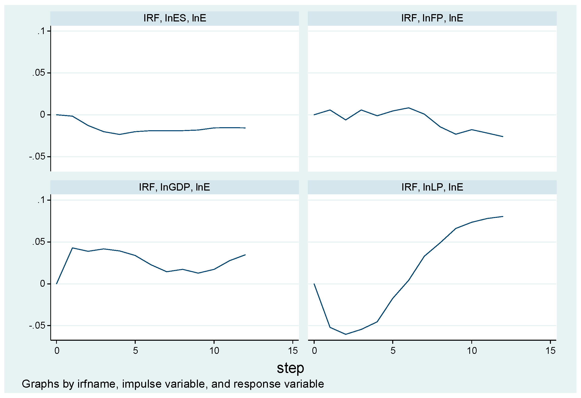
As shown in Figure 2, a positive impulse from the enterprise scale in the current period (namely the expansion of company size) will produce a negative response to energy consumption (namely a reduction of energy demand). In the early period, a positive impulse from fuel price causes a slight fluctuation in energy demand. However, in the long term, it will reduce energy demand. A positive impulse of GDP will cause an increase in energy consumption in subsequent periods. When labor productivity receives a positive impulse, it reduces energy demand at first, and then causes an increase in energy consumption later.

According to

Table 4. Forecast-error variance decomposition.

Results from IRF
	(1)	(2)	(3)	(4)	(5)
Step	Fevd	Fevd	Fevd	Fevd	Fevd
0	0	0	0	0	0
1	1	0	0	0	0
2	0.540930	0.003052	0.182242	0.273511	0.000265
3	0.570034	0.003027	0.143760	0.275967	0.007212
4	0.649489	0.002370	0.117521	0.216965	0.013655
5	0.700726	0.001621	0.102111	0.177573	0.017969
6	0.733684	0.001551	0.096968	0.147927	0.019869
7	0.751837	0.002149	0.092188	0.132020	0.021806
8	0.757523	0.001955	0.085875	0.131088	0.023558
9	0.746597	0.003770	0.081644	0.142912	0.025076
10	0.721234	0.008051	0.076266	0.168603	0.025846
11	0.694169	0.009989	0.072498	0.197552	0.025793
12	0.665529	0.012685	0.071822	0.224661	0.025302

(1) irfname = IRF, impulse = lnE, and response = lnE. (2) irfname = IRF, impulse = lnFP, and response = lnE. (3) irfname = IRF, impulse = lnGDP, and response = lnE. (4) irfname = IRF, impulse = lnLP, and response = lnE. (5) irfname = IRF, impulse = lnES, and response = lnE.

, besides the contribution of energy consumption itself, 22.466% of fluctuations in energy demand is attributed to labor productivity, and 1.269%, 7.182% and 2.530% of fluctuation in energy demand are attributed to fuel price, GDP and enterprise scale, respectively.

5. The Potential of Energy Conservation and CO₂ Abatement in China’s Machinery Industry

5.1. Estimation of Energy Demand and Forecast of Energy Conservation Potential

By analyzing the energy price index data, we know that the mean annual growth rate of the fuel price is about 6% during 2001–2013, and approximately 9% over the entire sample period. Taking the actual price levels and trends of all kinds of energy into account, the growth rate of fuel price is set to be: 6% as baseline scenario, 9% as advanced scenario and their mean 7.5% as medium scenario.

According to the National Bureau of Statistics, China’s GDP growth rate was 6.7% in the first three quarters of 2016. We therefore think it is also the same value in 2016. The Chinese government has formulated a GDP growth target of not less than 6.5% during the 13th Five-Year Plan period [50]. The Chinese Academy of Social Sciences conducted an analysis and outlook for the future macroeconomic situation predicting China’s GDP growth rate to be around 6% during 2021–2030 [51]. We set the GDP growth rates for the next 10 years based on the above information.

Table 5. The scenario of China’s GDP growth rates.

Variables	2017–2020	2021–2025
GDP	6.5%	6%

is the GDP growth rates during 2017–2025.

The 13th Five-Year Plan of the machinery industry requires the growth rate of labor productivity to reach 7.5%. It was set as a medium scenario. Meanwhile, we set 10% and 5% as baseline scenario and advanced scenario, respectively.

The average growth rate of enterprise scale is 5% during 2012–2013, and 11% during 2005–2013. The former is set as the baseline scenario; the latter as the advanced scenario; and the average of the two, 8%, as the medium scenario.

The above scenarios are summarized in

Table 6. The scenario assumptions of related variables.

Variables	Baseline Scenario	Medium Scenario	Advanced Scenario
FP	6%	7.5%	9%
LP	10%	7.5%	5%
ES	5%	8%	11%

.

The above scenario settings of the growth rates above are combined with China’s actual conditions and the judgment of economic theory, which are relatively reasonable.

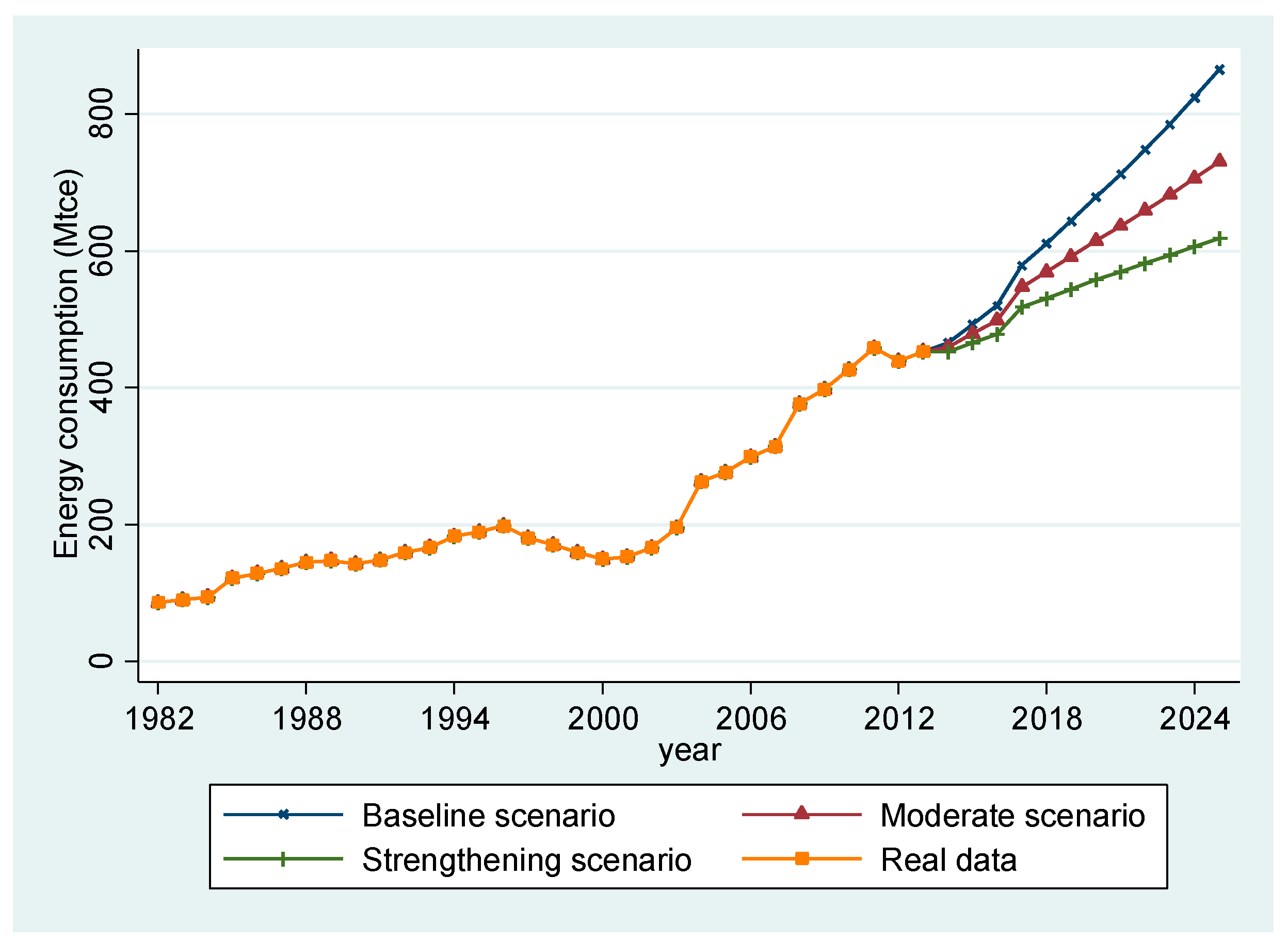
Under these three scenarios, we forecast the energy demand and conservation potential of energy in China’s machinery industry (see Figure 3).

According to the above-mentioned cointegration equation and growth rates of each variable, we predict energy demand in China’s machinery industry under different scenarios.

The forecasted results are displayed in

Table 7. The forecast of energy demand in China’s machinery industry (Unit: Mtce).

Year	Baseline Scenario	Medium Scenario	Advanced Scenario
2020	678.759	615.105	557.972
2025	865.494	731.055	618.547

.

As seen in Table 7, the predicted value of energy demand is 615.105 Mtce in 2020 under the medium scenario, which implies an energy-saving potential of 63.654 Mtce compared with the baseline scenario. The prediction is 731.055 Mtce in 2025 under the medium scenario, which implies an energy-saving potential of 134.439 Mtce, compared with the baseline scenario.

Under the advanced scenario, energy consumption in 2020 is about 557.972 Mtce, which implies an energy-saving potential of 120.787 Mtce compared with the baseline scenario. Energy consumption in 2025 is about 618.547 Mtce, which implies an energy-saving potential of 246.947 Mtce compared with the baseline scenario.

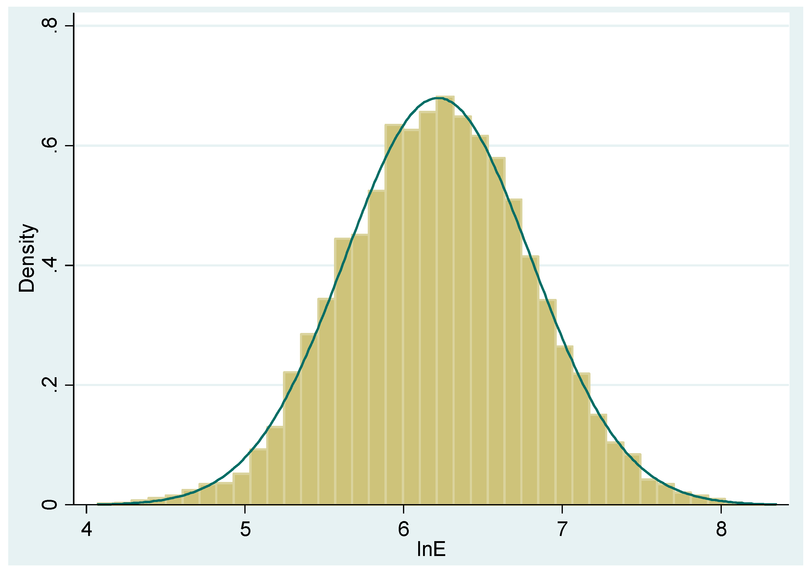
The Monte Carlo method is used to simulate energy demand in 2020 at a medium energy conservation scenario. It should be noted that, in the actual economic analysis, variables frequently appear in the form of natural logarithms. The differences between natural logarithms of a variable are the approximations of its change rates, while the change rates of a variable are generally stable sequences. According to previous experience, stationary series of an economic variable generally follows a normal distribution. To determine the parameters of the distribution of the independent variables, we obtained statistical characteristics of their change rates during 1983–2013 through simulation with Stata 14 (Stata Corp LP, College Station, TX, USA).

According to the mean and standard deviation from

Table 8. The description of variables.

Variable	Mean	Std. Dev.	Min	Max
ΔlnFP	0.075	0.085	−0.114	0.313
ΔlnGDP	0.065	0.025	0.037	0.141
ΔlnLP	0.075	0.170	−0.315	0.443
ΔlnES	0.08	0.253	−0.226	1.086

, specific forms of distribution for each independent variable can be obtained. There are 10,000 random numbers generated separately from the statistical indicators of each explanatory variable. Then, the energy demand in 2020 can be calculated according to the cointegration equation.

Table 9. The statistical characteristics of energy consumption of 10,000 random simulations.

Variable	Obs	Mean	Std. Dev.	Min	Max
lnE2020	10000	6.217	0.587	4.071	8.347

shows its statistical characteristics.

The mean is $\mu =6.217$, and the standard deviation is $\sigma =0.587$.

Its distribution is shown as Figure 4.

Therefore, the natural logarithm of energy demand in 2020 is $\ln E\in \left(\mu -\sigma ,\mu +\sigma \right)$, i.e., $\ln E\in \left(5.630,6.803\right)$, which is a reasonable range of predicted values. According to Table 7, the energy consumption may be 678.759 Mtce, 615.105 Mtce and 557.972 Mtce in 2020 under the baseline, medium and advanced scenarios, respectively, and their natural logarithms 6.520, 6.422 and 6.324 are within the forecasted range $\left(5.630,6.803\right)$.

5.2. CO₂ Emissions Forecast and Emissions Reduction Potential Analysis

Heat released by different types of energy is not the same, so in order to facilitate mutual comparison and research, the calorific value of 1 kg standard coal is defined as 7000 kcal. Standard coal is not a specific energy, but an energy unit of measurement with a uniform standard calorific value. With the change of energy structure, CO₂ emissions generated by a ton of standard coal may not be the same at different periods.

The less CO₂ emissions released by a type of energy, the cleaner that kind of energy is. From that perspective, hydropower, wind power, solar energy, and nuclear energy are much cleaner than fossil energy. Obviously, oil is cleaner than coal, and natural gas is cleaner than oil. Optimizing energy structure means improving the proportion of clean energy.

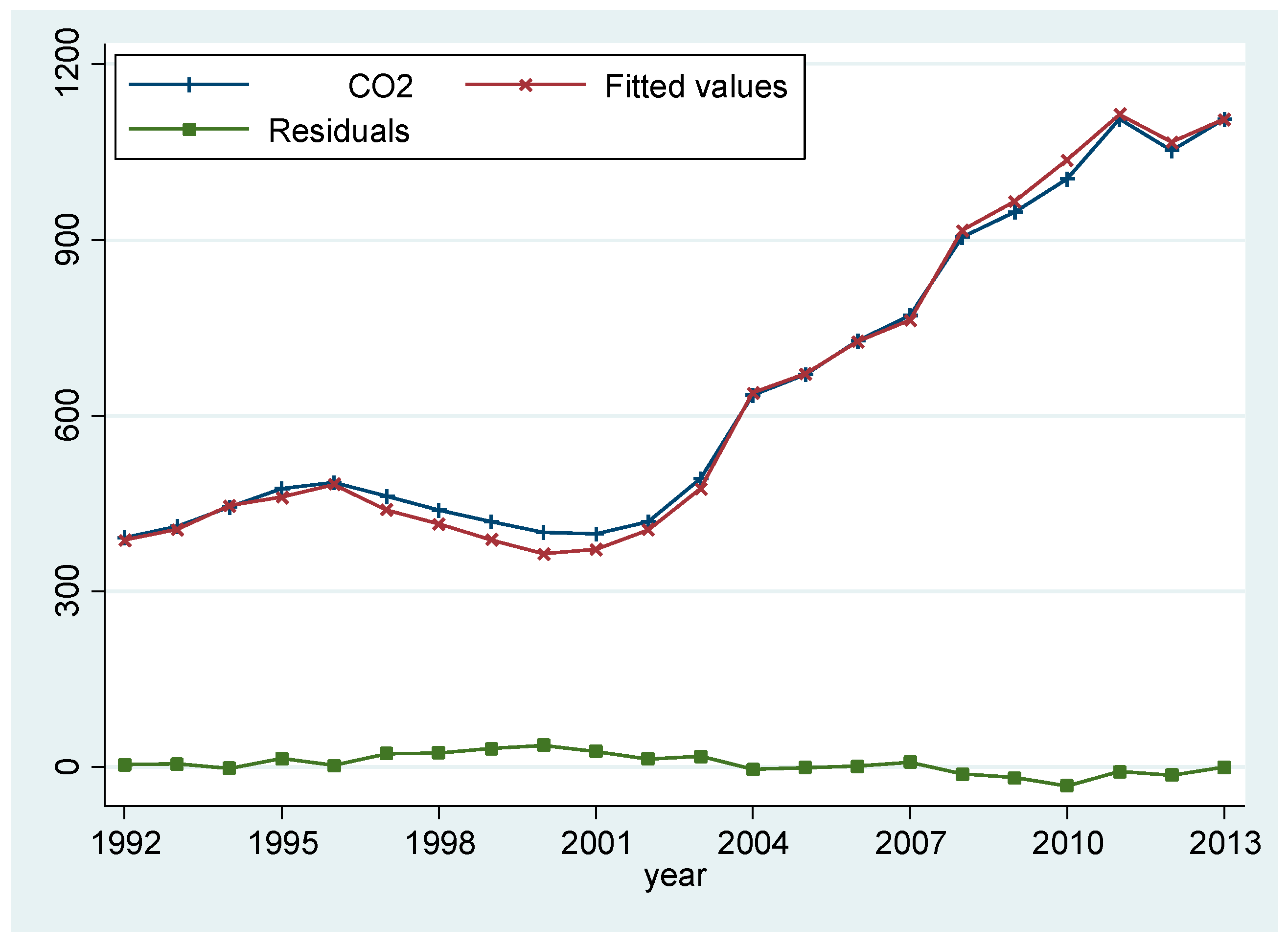
In 1992, China began its market-oriented economic reforms. In 1993, China became a net oil-importing country, rather than oil-exporting country. Therefore, we have reasons to believe that the issues of energy structure began to be highlighted in 1992, and since then, energy structure has been adjusted toward emissions reduction. This means that CO₂ emissions generated by a ton of standard coal are slightly decreasing annually. In other words, CO₂ emissions and time have a weak negative correlation. Therefore, to accurately predict CO₂ emissions, the data on energy and CO₂ emissions after 1992 are selected for analysis.

In the light of so many sources of energy, it is difficult to predict the consumption of different types of energy. We therefore only predict the total energy demand in China’s machinery industry. We adopt the method provided by Mi and co-workers [37,52,53] as well as Ang and Pandiyan [54] to estimate the corresponding CO₂ emissions based on historical data of different energy species and the algorithm in the 2006 IPCC Guidelines for National Greenhouse Gas Inventories (IPCC 2006) [55].

$$C{O}_2={\displaystyle \sum _i{E}_i\cdot A_i}$$

(7)

where, $E_i$ represents the consumption of fuel i; $A_i$, average CO₂ emissions coefficient of fuel $i$.

In addition, if no energy is consumed, there would be no CO₂ emissions. Thus, the constant term is discarded. The regression result is as follows:

$$\widehat{CO{2}_t}=2.433E_t-0.056\left(t-1992\right)$$

(8)

Environmental pressure prompted the adjustment of the energy structure, and the optimized energy structure is in favor of emissions reduction. It shows that the consumption of 1 Mtce energy will result in approximately 2.433 Mt CO₂ emissions, while continuing to optimize the energy structure will reduce 0.056 Mt CO₂ emissions per year on average.

As illustrated in Figure 5, CO₂ emissions had substantially been increasing in China’s machinery industry, which is mainly due to an increase in energy consumption. The Asian financial crisis of 1997 had a negative impact on China, which led to a reduction in energy consumption in subsequent years, thereby reducing CO₂ emissions. The fitting value and the actual value are basically consistent, and the residual fluctuates slightly around zero, which is in line with economic and econometrics theories.

Based on the energy consumption in the foregoing scenario analysis, CO₂ emissions corresponding to 2020 and 2025 are predicted under different scenarios (see

Table 10. CO₂ emissions forecast in China’s machinery industry. (Unit: million tons).

Year	Baseline Scenario	Medium Scenario	Advanced Scenario
2020	1649.73	1494.87	1355.88
2025	2103.75	1776.68	1502.97

).

In 2020, CO₂ emissions may be 1649.73 Mt (Million tons), 1494.87 Mt and 1355.88 Mt in the baseline, medium and advanced scenarios, respectively. CO₂ emissions in the medium scenario is 154.86 Mt less than that in the baseline scenario, and CO₂ emissions in the advanced scenario is 293.85 Mt less than that in the baseline scenario. In 2025, CO₂ emissions may be 2103.75 Mt, 1776.68 Mt and 1502.97 Mt in the baseline, medium and advanced scenarios, respectively. CO₂ emissions in the medium scenario is 327.07 Mt less than that in the baseline scenario and CO₂ emissions in the advanced scenario is 600.78 Mt less than that in the baseline scenario. Thus, reducing the consumption of fossil energy and optimizing energy structure have a significant influence on reducing CO₂ emissions and protecting the environment.

6. Conclusions and Policy Recommendations

We use the cointegration method to establish the long-term equilibrium relationship among fuel price, GDP, labor productivity, enterprise scale and energy consumption in China’s machinery industry during 1982–2013. We further predict the future energy demand in China’s machinery industry, and analyze the potential of energy conservation and CO₂ emissions reduction.

We forecasted the future energy demand in China’s machinery industry using scenario analysis which assumes that there is a wide variety of possible trends for each variable, thus resulting in diverse predictions. This method requires subjective imagination, emphasizing the predictor’s subjective desire in the future. Scenario analysis may not reflect the true state of the future. The correctness of the prediction and the quality of the scenario analysis depend on the establishment of the model and the choice of parameters. It relies on the past relationship and data, hence there are a lot of uncertainties.

Nevertheless, scenario analysis is still a feasible method in the absence of better options. It indicates that minimizing the future energy demand in China’s machinery industry may be achieved through energy-saving policies in a variety of energy-saving scenarios. Monte Carlo simulation verified the validity of prediction.

We predicted the future CO₂ emissions, which is based on the historical relationship between CO₂ emissions and total energy consumption as well as the expected energy consumption. However, the historical relationship and the expected energy consumption are estimates and predictions respectively, and not actual values. Therefore, the uncertainty is further increased. Despite these uncertainties and drawbacks, it can still provide a good reference for CO₂ emissions in China’s machinery industry.

The main conclusions and policy recommendations are as follows:

Firstly, a reasonable long-term cointegration relationship exists among fuel price, GDP, labor productivity, enterprise scale and energy consumption. The coefficients of all the explanatory variables are consistent with economic theory.

Secondly, a rising energy price reduces energy consumption. A 1% rise in energy price will lead to a 0.110% reduction in energy consumption. In China, the energy industry is essentially a state-owned monopoly, and energy price is set by the government. In order to maintain social stability and increase people’s welfare, the price set by the government is significantly lower than the competitive equilibrium price. Government pricing distorts the allocation of resources, which may lead to higher energy consumption. If supply and demand determines fuel price, resulting in fuel price increase, it will inevitably force enterprises to expand research and development (R&D) investment, and thus improve energy efficiency and save energy.

Thirdly, GDP has the greatest impact on energy consumption. A 1% rise in GDP will cause a 0.874% rise in energy consumption. With the continued growth of China’s GDP, the social demand for machinery products has been increasing, and hence the associated energy consumption. This rapid economic development directly led to the extensive growth and high energy consumption as well as CO₂ emissions in the machinery industry, which ignored the externalities of environmental pollution. The government should therefore impose an energy consumption tax, and the subsequent higher cost of energy may promote the substitution of capital and labor for fossil fuel and reduce energy consumption.

Fourthly, in this paper, higher labor productivity increases energy consumption. Urbanization and infrastructure construction in China have led to rigid social demand for machinery products. Higher labor productivity promotes the extensive growth of the machinery industry, which further requires the consumption of more energy. Of course, this only applies to some stages. With China’s economic restructuring and upgrading, and further development of the machinery industry, this phenomenon will be reversed.

Fifthly, the expansion of enterprise scale can also contribute to the reduction of energy consumption. If enterprise scale increases by 1%, energy consumption will be reduced by 0.289%. Expanding enterprise scale can optimize allocation of resources, improve the efficiency and rational use of energy, and reduce energy waste. Therefore, the government should encourage mergers and acquisitions in the machinery industry, and eliminate outdated small enterprises which are energy inefficient in order to effectively reduce energy consumption.

Climate and environmental issues have attracted worldwide attention. In 2015, nearly 200 parties agreed to the adoption of the Paris Agreement on Global Climate Change. The Paris Agreement requires all parties to jointly deal with the threat of climate change by stressing that the global average temperature rise should be maintained at 2 °C or less compared to pre-industrial levels. Meanwhile, the Chinese government made it clear that China’s CO₂ emissions would peak around 2030, and that striving to achieve this reduction goal as soon as possible is imperative [56]. The 13th Five-Year Plan put forward more strict requirements for energy and climate—i.e. for each unit of GDP, energy consumption and CO₂ emissions should be reduced to 15% and 18%, respectively. According to the 13th Five-Year Plan for energy conservation in the machinery industry, energy consumption per unit of industrial added value in 2020 should be reduced by 18% compared to that of 2015 [57]. The Chinese government should moreover promote market-oriented services such as contract energy management, cleaner production and energy auditing as soon as possible, and establish a sound energy-saving monitoring and technical service system for China’s machinery industry.

China’s current environmental pollution is closely correlated to industrialization. The machinery industry is highly energy consuming, and the proportion of coal in China’s energy infrastructure is very high. It is difficult to reconcile the contradictions among urbanization, industrialization and environmental protection. The government should formulate more effective policies and incentives for energy conservation and CO₂ emissions reduction through market mechanisms such as reforming energy prices and adjusting energy structure in order to force the machinery industry to adjust its industrial structure, develop a high-end machinery manufacturing industry, and eliminate obsolete and high energy-consuming machinery enterprises. At the same time, strict environmental standards and law enforcement are essential in order to prevent further deterioration of the environment. The improvement of environmental quality depends not only on the development of the economy and the perfection of the market mechanism but also on the formulation and implementation of environmental laws and regulations in addition to technical support.

In order to realize the energy conservation and CO₂ emissions reduction in China’s machinery industry under the medium and advanced scenarios, the corresponding combination of countermeasures should be to: establish environmental standards and emissions constraints; reduce energy intensity and improve waste recycling; and improve the competitiveness of clean energy for the replacement of fossil fuels. In addition, the government should levy environmental taxes based on the emissions level of machinery enterprises, encourage the machinery industry to reduce energy intensity, promote mergers and acquisitions of enterprises, and expand the scale of enterprises.

In summary, energy consumption in China’s machinery industry is increasing and the demand for energy has long been rigid. At present, energy intensity in China is much higher than that in Japan, which means that there is a large possibility for energy conservation in China’s machinery industry. The government should thus adopt appropriate policies and guide enterprises to actively promote energy conservation and minimize energy consumption. We recommend that the government subsidize and encourage enterprises to purchase highly efficient energy-saving equipment to stimulate energy saving and CO₂ emissions reduction in machinery manufacturing enterprises.