Carbon Reduction Strategies Based on an NW Small-World Network with a Progressive Carbon Tax


School of Economics and Management, Southeast University, No. 2 Southeast University Road, Nanjing 211189, China
*
Author to whom correspondence should be addressed.
Sustainability 2017, 9(10), 1747; https://doi.org/10.3390/su9101747
Submission received: 14 August 2017
/
Revised: 22 September 2017
/
Accepted: 26 September 2017
/
Published: 28 September 2017
(This article belongs to the Special Issue Carbon Footprint: As an Environmental Sustainability Indicator)
Abstract
:There is an increasingly urgent need to reduce carbon emissions. Devising effective carbon tax policies has become an important research topic. It is necessary to explore carbon reduction strategies based on the design of carbon tax elements. In this study, we explore the effect of a progressive carbon tax policy on carbon emission reductions using the logical deduction method. We apply experience-weighted attraction learning theory to construct an evolutionary game model for enterprises with different levels of energy consumption in an NW small-world network, and study their strategy choices when faced with a progressive carbon tax policy. The findings suggest that enterprises that adopt other energy consumption strategies gradually transform to a low energy consumption strategy, and that this trend eventually spreads to the entire system. With other conditions unchanged, the rate at which enterprises change to a low energy consumption strategy becomes faster as the discount coefficient, the network externality, and the expected adjustment factor increase. Conversely, the rate of change slows as the cost of converting to a low energy consumption strategy increases.
1. Introduction
Climate change, as an ultimate common problem of human beings [1], is caused by anthropogenic emissions of greenhouse gases such as carbon dioxide (CO2) that have serious ecological and economic consequences [2]. When considering the means to eliminate or reduce pollution, economists prefer market means because they are more efficient in both static and dynamic aspects [3,4,5].
Carbon tax and cap-and-trade systems have recently been introduced as general market-based carbon reduction measures [6,7]. The former stipulates the price of carbon emission permits, while the latter sets the quota for carbon emission permits. Price-type approaches are more effective and efficient than the quantitative approaches when dealing with public issues such as global warming [8]. Wittneben [9] mentioned that the uncertainties of the cap-and-trade system are due to not only supply and demand adjusting constantly to new information, but also political bargaining; any miscalculation or misrepresentation of party emissions will have a significant effect on the overall system. This is not the case for a tax: if the policy environment changes, it can be adjusted over time and it will not fluctuate as greatly as it would in a cap-and-trade system. In addition, construction and maintenance of a cap-and trade system require huge cost inputs, which a carbon tax does not (it is not difficult for the government to add a new tax). The cost of a cap-and-trade system is also more uncertain than the cost of a carbon tax: if economic growth is greater than expected, setting an upper limit on total emissions will limit economic growth and increase costs [10]. Thus, the carbon tax is more concise and implies lower management and economic costs than the cap-and-trade system.
However, the traditional single tax rate means that firms with different emission indexes adopt the same tax rate. This means that there are still disadvantages in terms of fairness and efficiency. A progressive tax rate is different: enterprises that pay attention to environmental protection receive low tax rates, and enterprises with high emission indexes receive high tax rates. Compared with the traditional single tax rate, this design is much fairer. Moreover, such a design can help enterprises improve production technology and increase the utilization ratio of production factors, which will contribute to the promotion of production efficiency.
Furthermore, studies that provide domestic theoretical descriptions and modeling of carbon tax policies are always based on their overall production and operation, which are relatively macroscopic and start from a completely rational perspective. However, the implementation of carbon tax policies depends on the cooperation of enterprises. Managers of enterprises usually have limited rationality and cannot adjust immediately. The strategy selection in evolutionary game theory is just of limited rationality. In addition, the process by which enterprises make decisions and policy adjustments is a dynamic, evolutionary process. In recent years, evolutionary games in the NW small-world network have advanced in solving the dynamic evolution of real problems [11,12]. The NW small-world network (Appendix A) creates the environment and the evolutionary game acts as a tool; the combination can help us better explain the application of progressive carbon tax policy in practice. Therefore, in this study we propose a new model for setting progressive carbon tax rates. Under the policy, the carbon tax is closely related to carbon emissions. We construct a progressive model of social welfare maximization, and set some model parameters to calculate the total emissions, product price, pre-tax profit, after-tax profit and the environmental costs of enterprises in certain industries, and draw relevant conclusions. Then, we construct the evolutionary game model with enterprises with different levels of energy consumption under an NW small-world network, and use it to study enterprises’ consumption strategy choices under the progressive carbon tax policy. Using experience-weighted attraction (EWA) learning theory and the relevant parameter settings, this study describes and simulates the dynamic strategy selection game between enterprises under the benchmark parameters. It also analyzes the influence of different parameters (including the discount coefficient, conversion cost, network externality and expected adjustment factor) on the evolution results. The results and conclusions can serve as a useful guide for governments to devise relevant policies and for enterprises to make strategic decisions.
2. Literature Review
The negative effects of greenhouse gas emissions are increasingly severe, and therefore carbon emissions are receiving more attention [13,14,15]. Nowadays, the two most popular carbon emission reduction regulation approaches around the world are the carbon tax and cap-and-trade. Cap-and-trade has attracted much more attention because of the emergence and development of the European Union Emissions Trading System (EU ETS). The EU ETS limits the annual aggregate emissions of carbon dioxide (CO2) by allocating a certain amount of pollution permits to each participating emitter. As the typical representative of the cap-and-trade system, the EU ETS not only significantly affects carbon emissions, economic performance and innovation [16], but also plays an important role in the stock market by introducing a “carbon premium” [17]. These advantages of cap-and-trade are worthy of recognition, but there are still many economists who believe that its shortcomings are more obvious and so prefer a carbon tax over cap-and-trade. Wittneben [9] discusses seven differences between carbon tax and cap-and-trade, and concludes that carbon pricing can be more cost-effective than a quantity instrument like ‘cap-and-trade’. Indeed, carbon tax can provide continuous emission reduction incentives to potential emissions without limit, lower transaction costs, and avoid rent seeking and speculative possibility [18], which are just the problems that cap-and-trade systems like EU ETS easily encounter [9].
We now turn to research on carbon tax. Jaeger [19] finds that climate change affects productivity and that the optimal environmental tax should be determined by marginal private damage. Bruvoll and Larsen [20] propose that the slowdown of Norway’s carbon emissions growth from 1990 to 1999 was mainly caused by changes in energy intensity and energy structure, rather than the introduction of carbon tax, which was ineffective due to wide-ranging tax exemptions. Floros and Vlachou [21] apply a two-stage translog cost function to illustrate that a certain amount of carbon tax is beneficial to Greece’s emission reduction activities. Callan et al. [22] study the effects of carbon tax in the Republic of Ireland and conclude that if the tax revenue is used to increase social benefits, the income gap will narrow. Bureau [23] analyzes the impact of carbon tax on different income groups using panel data and finds that the tax is beneficial to the poor, regardless of whether it is in accordance with the number of households or the number of people. Wesseh and Lin [24] propose a set of optimal emissions fees that could be used to reduce the damage caused by industrial pollution, and their results suggest that constructed optimal pollution taxes range from as high as 2.9% per dollar of output for heavy manufacturing in high-income countries, to as low as 0.01% in the service sectors of low-income countries. Liu et al. [25] analyze Chinese companies’ preferred design options for a carbon tax policy. Most of these studies discuss the intensity of the carbon tax policy, the factors affecting the policy under a particular goal orientation, and the impact of the policy on the economy. However, little attention is given to the innovation of carbon tax policies from the perspective of the carbon tax rate.
Numerous studies have proposed the concept of progressive tax. Yates [26] points out the importance of progressive taxes for universal health problems. Chiroleu-Assouline and Fodha [27] reveal the consequences of different environmental tax policies and propose the idea of tax reforms, from regressive pollution taxes to progressive environmental taxes. Orsi [28] believes that one way to achieve sustainable development is to impose a progressive tax on consumer goods, especially those that have adverse effects on the environment. Therefore, progressive tax is an improvement on traditional tax policies, and on this basis we propose the concept of a progressive carbon tax and model it.
At the same time, research on evolutionary game theory has matured. The earliest result using evolutionary game theory was the explanation of group behavior in the Nash equilibrium, which was proposed by Nash in 1950. The evolutionary stable strategy was introduced in the 1970s [29,30]. Taylor and Jonker [31] put forward another important concept for evolutionary game theory, named replicator dynamics. Evolutionary game theory has since developed rapidly and has been applied in many disciplines. For example, Ji et al. [32] build on the supplier selection model and use an evolutionary game model to explore the cooperation trend between multiple stakeholders to establish long-term interest relationships for green procurement between stakeholders (suppliers and manufacturers). The application of evolutionary game theory as a tool is also being used more broadly. Nevertheless, the study of carbon tax is mainly based on the general equilibrium model [33,34,35], and evolutionary game theory is rarely applied. However, the application of evolutionary game theory can better explain how enterprises make decisions and how the enterprises in certain areas interact with each other in the implementation of the carbon tax policy.
We adopt the following research methods in this study. First, we establish a progressive carbon tax model based on carbon tax rates and carbon emissions and propose a social welfare maximization model to evaluate the utility of the carbon tax policy. We also introduce the NW small-world network theory and game theory and apply them to the field of carbon tax. A complex network system based on an NW small-world network is constructed and an experience-weighted attraction (EWA) learning model is selected to simulate and analyze the evolutionary game between different enterprises in the industrial cluster under the progressive carbon tax policy. With policy diffusion in certain conditions, we analyze how the enterprise discount coefficient, purchase price, network effects and expectation influence the application of the policy. The results provide a reference for the real application of carbon tax policies and enterprise strategies. In particular, this study proposes the concept of a progressive tax rate, and combines social welfare maximization, evolutionary game theory, EWA learning theory, and NW small-world network theory to elaborate the problem. The combination of multiple disciplines makes the research conclusions more generalizable.
3. Research Method and Model Construction
3.1. Progressive Carbon Tax and Social Welfare Maximization Models
3.1.1. A Model of Progressive Carbon Tax Policy
Assume that there are N companies in a certain traditional industry, each producing a single type of homogeneous product, and their outputs are . Carbon dioxide emissions are mainly produced by burning fossil fuels to meet the energy needs for production. If company needs energy to produce one unit of product, the energy that it needs to produce products is
where represents the fuel type code, represents the energy consumed per unit of fuel l, and is the amount of fuel l consumed by company i.
Carbon dioxide emissions can be calculated using the emission index to convert energy consumption data. The average value of the CO2 emission index during production reflects the amount of emissions per unit of production. Therefore, the CO2 emission index during the production process of company i can be calculated as
The emission factor varies for each company to reflect the differences in their production efficiency and levels of technology. The total CO2 emissions originating from fossil fuels are calculated as , where represents the CO2 emissions when company i uses one unit of fuel l. Thus, the CO2 emission index of company i is
Policy-makers would prefer to develop a carbon tax that has a minimal effect on the economy while achieving the goal of reducing emissions in a given industry. It is assumed that the regulatory authorities set the target emission factor for a particular industry, and when the level of CO2 emissions differs, different levels of tax should be imposed.
When the carbon emission index of company i is , the n-level progressive tax rate for this company is
Formula (4) shows that for the company’s production and operation activities, the carbon tax rate and the CO2 index are positively correlated; that is, the higher the CO2 index, the higher the tax burden on companies at the corresponding emission level.
3.1.2. Social Welfare Maximization Model
Assuming that the environmental cost of company i’s production activities is , under the progressive carbon tax policy, is
Formula (5) indicates that under the progressive carbon tax policy, the environmental costs are also progressive. The higher the level of emissions, the higher the environmental cost of the enterprise’s production and operation activities.
Assuming that the number of products produced by company i is qi and its production capacity limit is , then the enterprise production cost function is the quadratic function ( and are known constants).
Assume that the fuel cost of company i is , where is the unit cost of fuel l and is the amount of fuel l consumed by company i.
The producer surplus maximization model of company i is
Function (6) maximizes the surplus of company i and depicts its profit structure; is the income from selling products to consumers; is the sum of the production cost and the fuel cost; and is the environmental cost. Constraint condition (7) ensures that the number of products produced is under the production capacity. Constraint condition (8) is the energy conservation formula. Constraint condition (9) indicates the CO2 emission factor. Constraint condition (10) is a non-negative constraint to guarantee the non-negativity of the parameters.
Assuming the environmental cost , then is
The producer surplus maximization model can be rewritten as
Constraints (16)–(18) ensure that the environmental cost of the enterprise is non-negative under the progressive carbon tax policy.
The consumer surplus is the difference between the expected price and the actual price paid by the consumer. The consumer surplus can be calculated using the demand function integral minus the price paid to the enterprise [36,37]. In a perfectly competitive market environment, the inverse demand function is , where is the intercept, is the slope of the inverse demand function, and is the total market demand for products.
The consumer surplus is
The market clearing condition is
Market clearing means that the price of the commodity has enough flexibility to meet the demand and adjust the balance of the market supply. In a perfectly competitive market, Pareto optimality is achieved when the market clearing condition is satisfied, which maximizes the social efficiency. A change in the production level reduces the total social efficiency, which reduces the producer surplus. In such a market, it is helpful to study the utility of the carbon tax policy through the social welfare maximization model.
The market clearing condition is used to ensure that all industrial requirements are met. In a market equilibrium model where consumers and producers are perfectly competitive price-takers, social welfare can be represented by the consumer surplus and producer surplus models (detailed analysis is provided in Appendix B), constrained by consumers, producers and market clearing conditions [37].
The social welfare maximization model is
3.2. Evolutionary Model of Traditional Industrial Clusters Based on a Progressive Carbon Tax Policy in a NW Small-World Network
3.2.1. Evolutionary Game Learning Model
This model uses EWA learning theory [38]. The strategy game between enterprises is established and the formula for updating empirical weight Mt is
where is the discount factor of experience, which reflects the learning speed of the enterprises. , the attractiveness index of strategy j for individual i in period t, is calculated as
where φ is the discount factor of the past attraction index, reflecting that the strategic attractiveness decays during the game. The EWA learning model controls for the growth of the attractiveness index through the parameters and φ, which reflect the participants’ learning speed. is an indicative function, and is the practical strategy of individual i. When , = 1. μ is the discount factor for the income of the non-choice strategy, where a higher value of μ shows that the enterprise pays more attention to the strategy. indicates the benefit that individual i gains by selecting strategy j when other individuals select strategies during period t. Based on the study by Xian and Mei [39], we set the expected earnings as , the numerical value of which depends on how individual i expects his game opponent to behave in period t. In the EWA learning model, the attraction index of each strategy determines the probability that strategy j is chosen: the greater the attractiveness index, the higher the probability. Let be the number or proportion of opponents of individual i in state k in period t. In each period, individual i adjusts his expectation for the behavior of his opponent according to the actual situation. The adaptive expectation adjustment equation is
where is the number or proportion of game opponents of individual i in state k in period t − 1, and is the expected adjustment factor, with larger values indicating faster adjustment. The equation can be rewritten as
In the EWA model, every strategy has its own appeal index that determines the probability that it is randomly chosen. The higher the appeal index, the more likely it is that the strategy will be chosen. A logit decision model is applied to calculate the probability that strategy j will be chosen by individual i in period t,
where is the sensitivity of the attractiveness index in strategic decision-making, which is used to judge the rationality of decision-makers.
3.2.2. The Basic Premise of the Traditional Industrial Cluster Evolution Model
Premise 1.
In the real economy, there is an area in which all enterprises manufacture homogeneous products. There is market competition and a strategy game among them. There are no enterprises producing homogeneous products in the surrounding area, so the strategy game only exists within the region. The progressive carbon tax system is implemented in this region.
Premise 2.
All enterprise agents have limited rationality; under normal circumstances, enterprises base their decisions on the expected returns, but sometimes they make mistakes, which is consistent with the reality.
Premise 3.
Ignoring other factors, it is assumed that the cooperative game among enterprises has only three levels of energy consumption: high, medium and low. We do not take into consideration the specific energy differences at a certain level of energy consumption.
3.2.3. The Expected Earnings Setting in the Evolutionary Game
Set up enterprise i in period t and choose the strategy ,
the high, medium and low energy consumption strategies refer to the characteristics of the production equipment.
The expected return function is
where represents the expected earnings foreign to the network externalities when selecting plan j, and . represents the expected return when enterprise i takes strategy j in period t; . is the discount factor, representing the importance of the enterprise’s future earnings; and is the expected environmental cost when enterprise i takes strategy j in period t.
When the enterprise takes strategy j in period t, it is expected to obtain the return , which is compatible with strategy k.
is the network effect parameter for strategy j, and the higher the value, the larger the network effect; β is the network effect index, which is exogenously given as β > 1 to ensure that the second order derivative of the network effect earning function is less than zero. is the compatibility coefficient of strategy j and strategy k, where the higher the value, the greater the revenue. Assuming that the same strategies are fully compatible, that is, the compatibility coefficient is 1, and different strategies are partially compatible, then the compatibility coefficient matrix between the three strategies can be written as
and . indicates the number of agents that enterprise i expects to adopt strategy k in its neighborhood in period t. Enterprise i adjusts its expectations each period according to the actual situation. The adaptive expectation adjustment equation is
where is the number of enterprises adopting strategy k in period t1 in the neighborhood of enterprise i, and is the expectation adjustment factor.
In period t, enterprise i is expected to obtain the network externality return if it adopts strategy j, which is the sum of the compatibility gains of enterprise i and all of the other enterprises in its neighborhood:
is the purchase cost when enterprise i takes strategy in period t − 1, and takes strategy j in period t. It is assumed that there is no purchase cost when the same strategy is chosen, whereas there are certain purchase costs when a different strategy from that in the previous period is chosen. Therefore, under different conditions, the purchase cost can be written in matrix form
where . is the expectation of the environmental cost when enterprise i takes strategy j in period t.
3.2.4. The Evolution Mechanism of Enterprises under the Progressive Carbon Tax Policy
In the first stage, each enterprise adjusts its probability of achieving every state after adopting a high, medium, or low energy consumption strategy, using the adaptive expectation adjustment method based on the environmental cost of the progressive carbon tax policy. The expected return when adopting the different strategies can then be calculated.
In the second stage, the method of adaptive expectation is used to adjust the number of enterprises in the neighborhood that will adopt the three energy consumption strategies, and the corresponding network externalities are calculated.
In the third stage, according to the EWA model, the attractiveness index and the probability of being chosen are updated for each of the three strategies, and the company acts according to the probability.
From the evolutionary analysis, we obtain the number of enterprises adopting each of the three strategies under the progressive carbon tax policy. We also obtain the evolutionary results for enterprises’ choices of different energy consumption strategies. Then, we study how the evolution results are affected by different parameter settings, allowing us to provide some suggestions for the application of the progressive carbon tax policy in real life.
4. Numerical Simulation and Results
4.1. The Solution of the Progressive Carbon Tax and Social Welfare Maximization Model
In the model solution, we consider enterprises with high, medium and low levels of energy consumption. These refer to the characteristics of the production equipment, which represent the difference in energy consumption for a unit product. The higher the value of , the higher the energy consumption of enterprise i. In addition, the higher the energy consumption of enterprise i, the lower the marginal cost of production, which is consistent with the actual operation of enterprises. We assume that companies can use coal, petroleum coke and natural gas as fuel. We use data sources from Natural Resources Canada (NRCan) and the US Environmental Protection Agency (EPA). According to the 2007 report by the International Energy Agency, we choose the ceramic industry to determine the average energy consumption per ton of clay production and the ratio of clay to finished ceramics. The parameters for fuel and production process are shown in Table 1 and Table 2.
For the inverse demand function, and are set to 376 and 0.0376, and and are set to 0.3 and 0.4 (Appendix C). When the price is 0, the market demand is 10,000 tons, which is higher than the production capacity limit of the enterprise. The reduction in carbon emissions at different levels can be achieved by adjusting the value of the rate r.
The progressive tax rate is divided into three levels to solve the model. Set the zero level tax rate as , the first level tax rate as , and the second level tax rate as and . ranges from 0 to 50 and from to 50. Now, we can solve the emission indices and calculate the emissions for high, medium and low energy consumption enterprises, as shown in Figure 1, Figure 2 and Figure 3. (This part is solved by Matlab.).
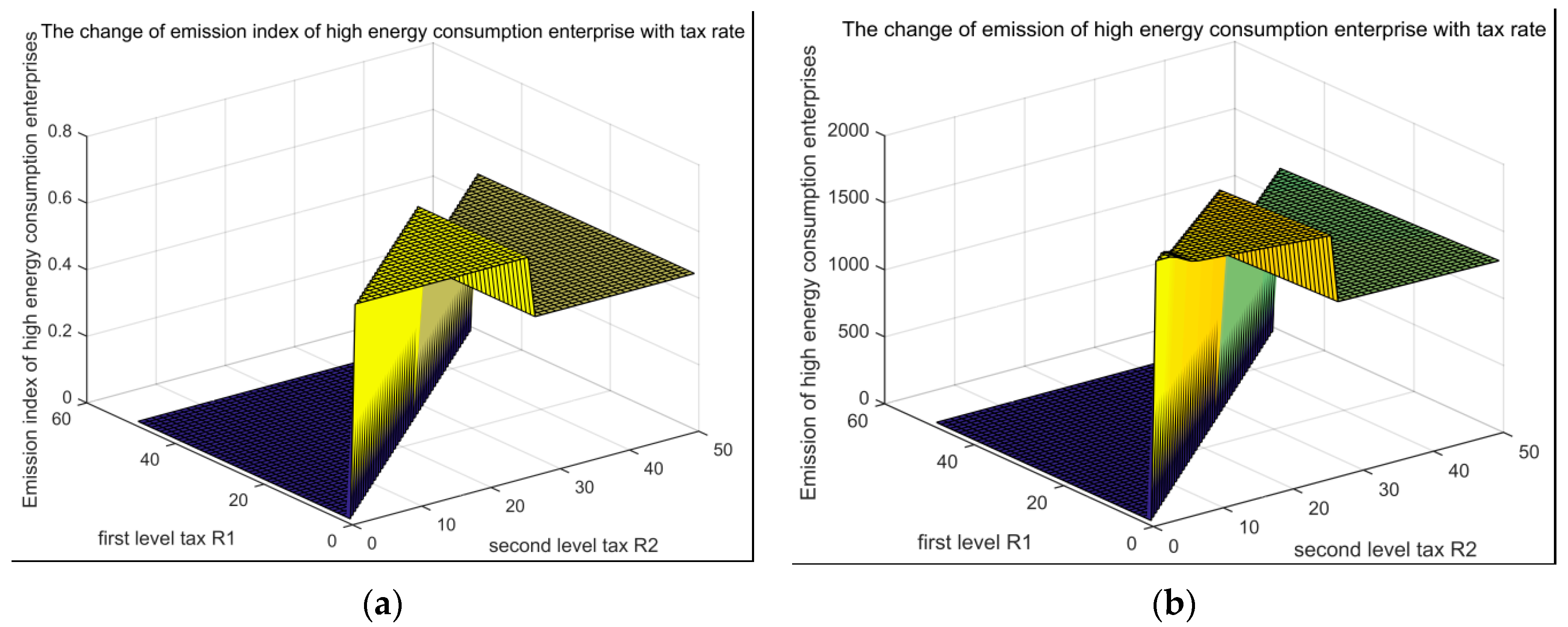
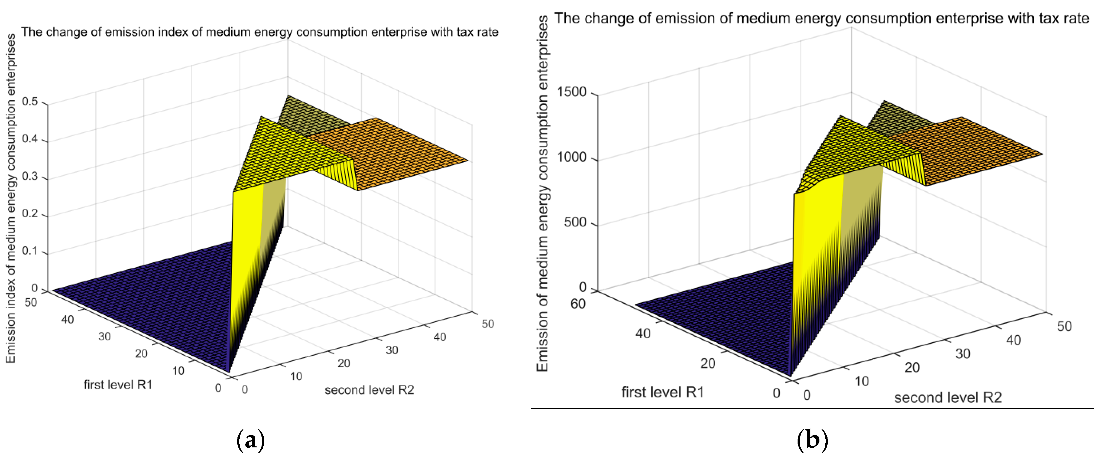
The emission index and emissions are at their lowest levels when and for high energy consumption enterprises (Figure 1), when and for medium energy consuming enterprises (Figure 2), and for low-energy enterprises (Figure 3). We consider to calculate the emission factors, emissions, environmental costs, pre-tax profits, and after-tax profits of the three types of enterprises, as shown in Table 3.
Table 3 shows that high energy consumption enterprises have the highest emission factors, emissions, and environmental costs, and the lowest pre-tax and after-tax profits, while low energy consumption enterprises have the lowest emission index, emissions and environmental costs and the highest pre-tax and after-tax profits.
4.2. Evolution of Enterprises under the Progressive Carbon Tax Policy
4.2.1. Parameter Initialization Settings
An NW small-world network is used to establish a multiple-agent system to analyze the adoption of different energy consumption strategies in the industrial cluster under the progressive carbon tax policy over time. The game is evolutionary and circulates T times after the parameter initialization. Considering that the traditional industrial cluster contains a large number of enterprises, we set the total number of nodes in the network as N = 1000; half the number of neighboring nodes for each node in the nearest neighbor coupling network as K = 3; the random border probability as p = 0.01; the discount factor of the past attraction index as ; the past experience of the discount factor as ; the discount factor of the non-choice strategy as ; the sensitive factors in strategic decision-making as ; the evolutionary length as T = 30; the network effect parameter as ; and the prices of the three strategies as , and . The compatibility coefficients are , and . The expected earnings are unrelated to the network externalities of the three energy consumption strategies, , , and . The environmental costs of the three energy consumption strategies are , , and . As the emission coefficient, environmental cost and profits were calculated above, we do not calculate them again here. Instead, the profits before tax and environmental costs of the three strategies are replaced by simple numbers. The discount coefficient of enterprises is , the network effect index is β = 2, the expected adjustment factor is ξ = 0.5 and the initial experience weight is .
4.2.2. Evolution among Enterprises under the Benchmark Parameters
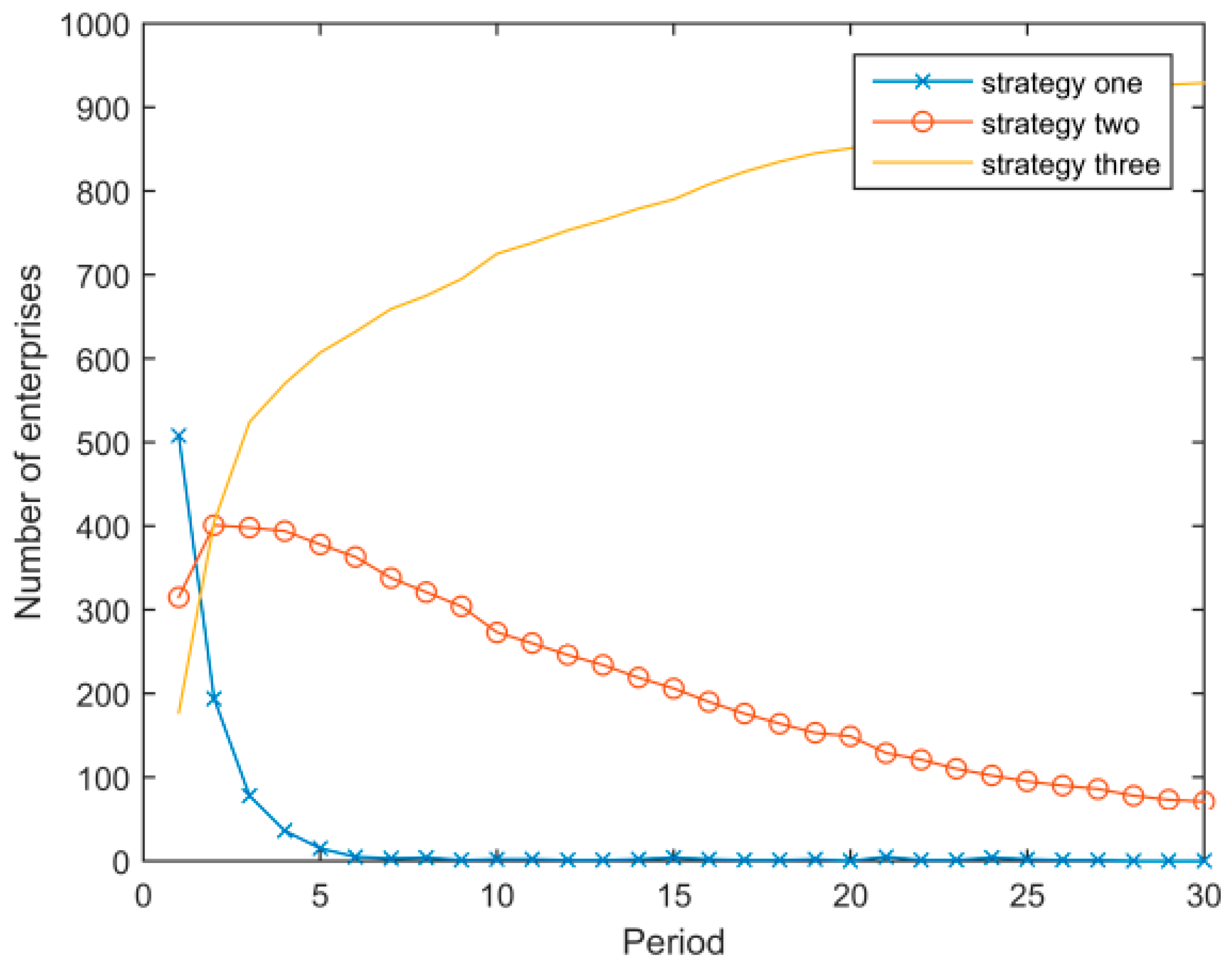
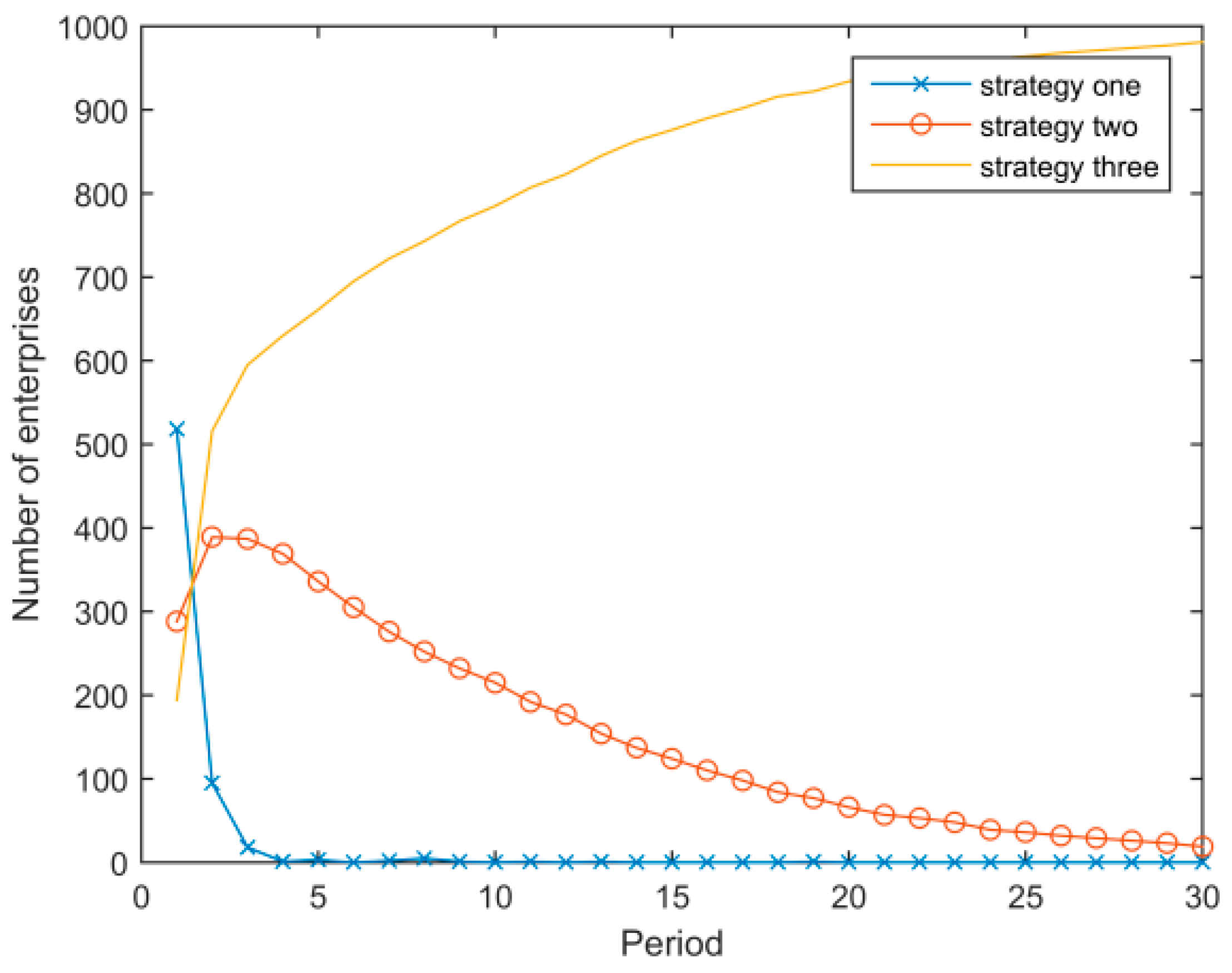
We assume that the initial proportions of enterprises adopting the three energy consumption strategies are 0.5, 0.3, and 0.2, respectively. In the Matlab simulation tests, the results for the number of enterprises adopting the three strategies in the system are shown in Figure 4. In the initial situation, the high energy consumption strategy has the most adopters but the number sharply decreases to zero during the evolution; the number of enterprises that adopt the medium energy consumption strategy increases at first, then decreases to zero; and the number of enterprises that adopt the low energy consumption strategy gradually increases to all those in the system. Although converting from a higher to a lower energy consumption strategy involves extra costs, the lower consumption strategy enjoys higher profits and lower environmental costs. Thus, all of the enterprises in the industrial cluster gradually change to the low energy consumption strategy. The network externalities also facilitate the evolution of the industrial cluster. Under the influence of straight network externalities caused by the link preferences of the NW small-world network, when some of the enterprises in the network adopt a strategy, it will improve neighboring enterprises’ income expectation for the strategy, thus driving them to adopt it faster and facilitating the rapid evolution of the industrial cluster toward the strategy. Therefore, as the number of enterprises adopting the low energy consumption strategy increases, it raises the income expectation not only of the enterprise but also of the network externalities, thus attracting more enterprises to adopt the low energy consumption strategy.
4.2.3. The Influence of Parameter Values
The following analyses examine how the parameter values affect the evolution of the industrial cluster. Keeping the other parameters at their baseline values, we change the discount coefficient of enterprises , the price of the low energy consumption strategy , the network effect parameter , and the expected adjustment factor ξ, respectively, to explore how the industrial cluster evolves.
- (1)
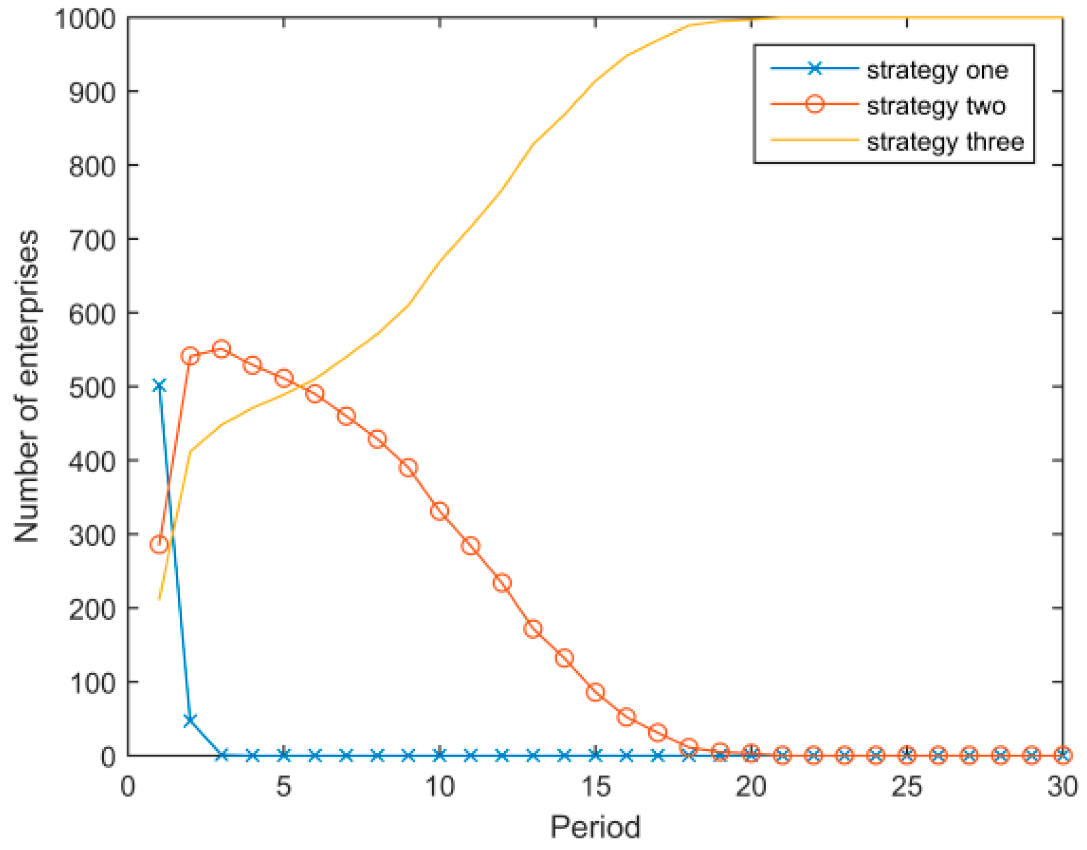
- Assuming that other parameters remain unchanged, Figure 5 and Figure 6 show the evolution results when the discount coefficient of enterprises is δ = 0.1 and δ = 0.9, respectively. Figure 5 illustrates that when δ = 0.1, the general evolutionary trend of the system remains unchanged, but the evolution is slower than with the baseline parameter (δ = 0.5). Figure 6 illustrates that when δ = 0.9, there is a “boom” phenomenon that diffuses the low energy consumption strategy to the whole system.
From Figure 4, Figure 5 and Figure 6, we conclude that while other parameters remain unchanged, the greater the discount coefficient of enterprises, the faster they change from the high to the low energy consumption strategy. The reason for this is that enterprises attach more weight to their future earnings, so there is greater emphasis on how the environmental costs arising from production activities affect profits. Thus, the government should make efforts to publicize the economic advantages of the low energy consumption strategy, so that enterprises can pay more attention to the higher profit and lower environmental cost of the low energy consumption strategy. In this way, high and medium energy consumption enterprises will place more emphasis on future earnings and speed up the transition to a low energy consumption strategy.
- (2)
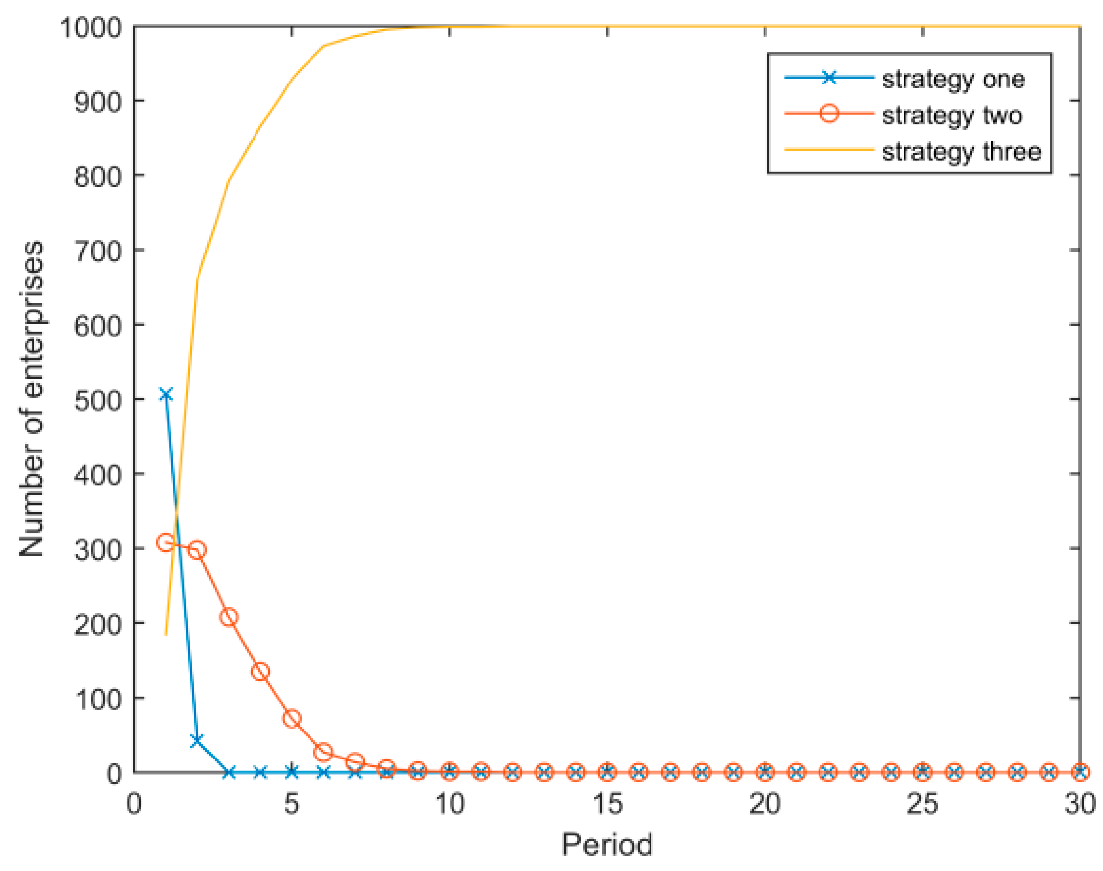
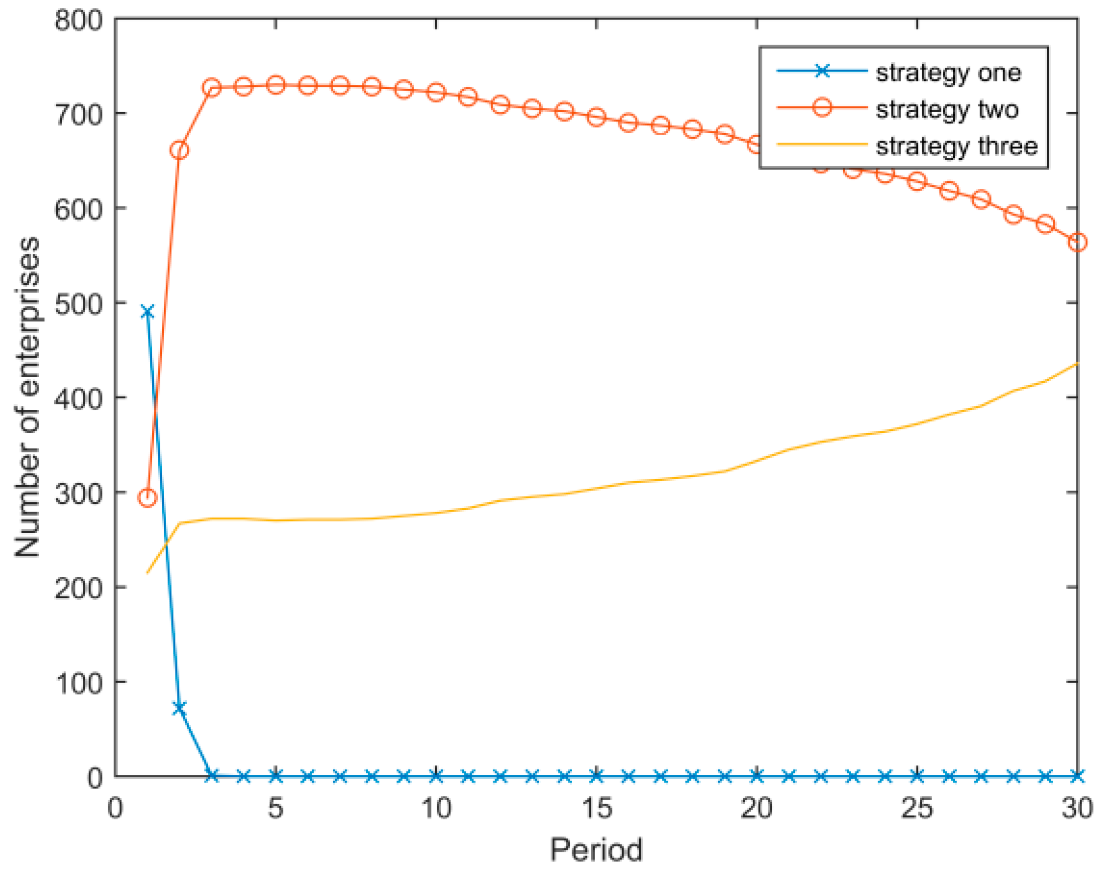
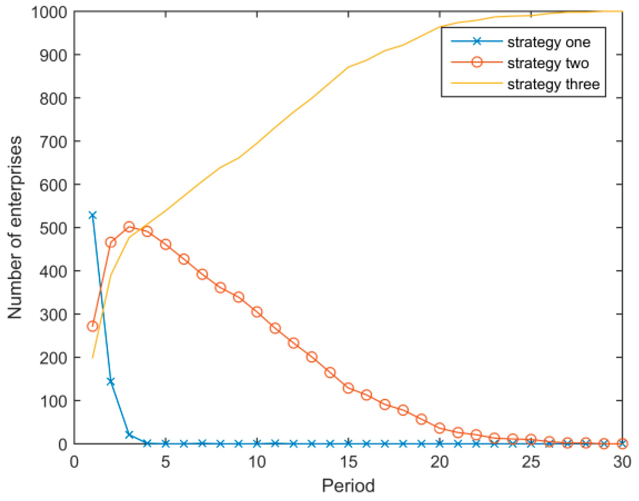
- Assuming that other parameters remain unchanged and only the price of the low energy consumption strategy changes, Figure 7 and Figure 8 show the evolutionary result when and , respectively. Figure 7 illustrates that when , the low energy consumption strategy is diffused much faster, and even the number of enterprises adopting the medium energy consumption strategy does not increase during the process of evolution. Figure 8 illustrates that when the price of the low energy consumption strategy is high, enterprises with a high energy consumption strategy initially convert to the medium energy consumption strategy, and the low energy strategy cannot spread across the system.
Comparing Figure 4, Figure 7 and Figure 8, we conclude that the lower the cost of converting to the low energy consumption strategy, the higher the diffusion speed. When the conversion cost reaches a certain value, the low energy consumption strategy will not spread to the entire system. Thus, the government can provide subsidies to the enterprises that are implementing transformation to the low energy consumption strategy. For example, the government can subsidize enterprises that buy new environmentally-friendly production equipment to replace their old equipment. This can encourage high and medium energy consumption enterprises to transfer to low energy consumption strategy more quickly.
- (3)
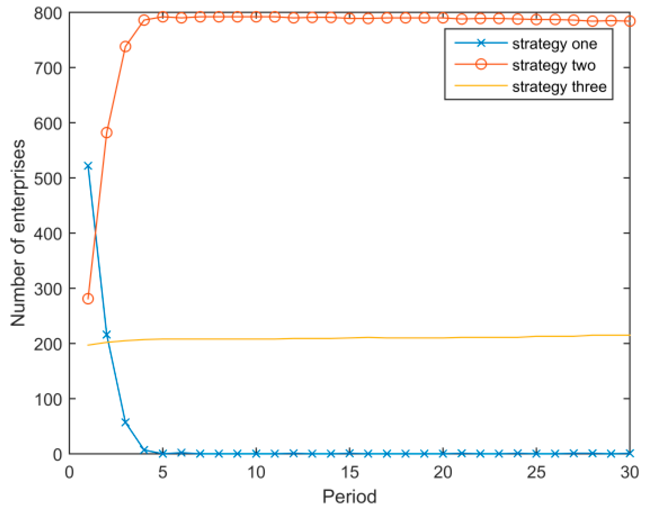
- Figure 9 shows the system evolutionary result when the network effect parameter is changed to , and Figure 10 when . Figure 9 illustrates that when the network externalities are small, the evolutionary trend is similar to that with the baseline parameter, but the speed is slower. Figure 10 illustrates that when the network externalities are large, the low energy consumption strategy eventually spreads to the whole system, but there is a period during which the medium energy consumption strategy dominates.
Combining Figure 4, Figure 9 and Figure 10, we conclude that large network externalities are beneficial to the diffusion speed of the strategy. Figure 10 illustrates that the medium energy consumption strategy has an initial advantage because of its higher initial network externalities, while the low energy consumption strategy gradually takes over from the medium energy consumption strategy because of its higher profit and lower environmental costs. The government can moderately help establish more low energy startups, thereby enhancing the externalities of low energy consumption programs, and then attracting more high energy consumption and medium energy consumption enterprises to adopt low energy consumption programs.
- (4)
- With other parameters unchanged, the expected adjustment factor ξ is set respectively to 0.1 and 0.9. The evolutionary results are shown in Figure 11 and Figure 12. Comparing these two figures with Figure 4, we conclude that the larger the expected adjustment factor, the higher the diffusion speed of the low energy consumption strategy. When the enterprises have a certain expectation for a standard, the faster adjustment quickly reduces the initially large number of enterprises adopting the high energy consumption strategy. The government should increase the publicity for successful examples of the transition to low energy consumption strategy, thereby making those high energy/medium energy enterprises become more confident in the transition to low energy consumption strategy, rather than let them think that it is a “difficult” process which requires significant time and money to complete.
5. Conclusions and Discussion
Given the lack of studies exploring innovative carbon tax policies, we propose a progressive carbon tax policy and build a social welfare maximization model on this basis. We solve and analyze the model to calculate the environmental costs of high, medium and low energy consumption enterprises, their pre-tax profits, after-tax profits, and other indicators. We analyze the strategy selections of enterprises in the industrial cluster using mathematical modeling, evolutionary game theory, EWA learning theory, NW small-world network theory and Matlab modeling and simulation methods.
The main conclusions are as follows.
- (1)
- Under the progressive carbon tax system, enterprises initially adopt different energy consumption strategies and gradually switch to the low energy consumption strategy, which eventually spreads to the entire system. There are two reasons for this result. First, the low consumption strategy has higher profits and lower environmental costs, so the benefits cover the cost of transitioning from a high to a low energy consumption strategy. Second, due to the influence of network externalities, when a business entity chooses a low consumption strategy, neighboring enterprises increase their expected income from adopting a low energy consumption strategy, thus driving the agents in the neighborhood to adopt the strategy faster.
- (2)
- With other conditions remaining unchanged, the greater the discount coefficient of enterprises, the faster they will change to a low energy consumption strategy. Because companies pay more attention to future earnings, they pay more attention to how the environmental costs arising from production activities affect their profits.
- (3)
- The higher the cost of converting, the longer it takes for enterprises to change to a low energy consumption strategy. When the conversion cost is higher than a certain value, the low energy consumption strategy will not spread to the entire system because the cost is higher than the expected benefit. In this case, enterprises that previously adopted the high energy consumption strategy will change to the medium energy consumption strategy.
- (4)
- The network externality effect is positively associated with the diffusion speed of the low energy consumption strategy. When the network externality effect is large (but not too large), the advantages of the low energy consumption strategy gradually rise and the strategy quickly spreads to the whole system because of its higher profit and lower environmental costs.
- (5)
- The greater the expectation adjustment factor, the faster the diffusion speed of the low consumption strategy. This is due to the rapid reduction in the number of enterprises that initially adopt the high energy consumption strategy when the expectation adjustment speed is faster.
Therefore, the low energy consumption strategy becomes the norm within the industrial cluster because the lower environmental costs enable enterprises to maximize their profits. For enterprises, this situation should speed up the development of technological innovations for low energy consumption to achieve carbon emission reductions, which also maximizes their own interests. For the government, the formulation of relevant policies should take full account of the effects of multiple factors on social welfare. Carbon tax policy-related indicators should be adjusted to maximize social welfare to achieve emission reduction targets that minimize the policy’s limitations on economic growth while simultaneously maximizing its benefits.
With respect to the process of the game between enterprises, this paper mainly considers the expected revenue function constructed by combining economics with NW small-world network theory in the process of enterprise strategy selection. The influences of specific layers in enterprises’ operations (such as production and inventory) on strategy selection are worthy of further study. Although the models are also suitable for the analysis of other traditional industries, it will be necessary to use long-term and multi-industry data to conduct more empirical analysis in the future.
Acknowledgments
This research was supported by the Humanities and Social Sciences Foundation of China Ministry of Education (No. 14YJA630066) and the Special Fund for basic research business of Southeast University in 2017 (No. 3214007113).
Author Contributions
B.W. had the idea and conceived the concept of the article; W.H. and P.L. built models and performed the numerical simulation; and W.H. was responsible for the overall writing process.
Conflicts of Interest
The authors declare no conflict of interest.
Appendix A
An introduction to the NW small-world network model:
- (1)
- To learn about the NW small-world network, let us start with the WS small-world network. The first small-world network model (WS small-world network model) was proposed by Watts and Strogatz [40]. Ordinarily, the connection topology is assumed to be either completely regular or completely random. However, many biological, technological, and social networks lie somewhere between these two extremes. Thus, they explored simple models of networks that can be tuned through this middle ground: regular networks ‘rewired’ to introduce increasing amounts of disorder. These systems can be highly clustered, like regular lattices, yet have small characteristic path lengths, like random graphs.
- (2)
- However, there is an obvious disadvantage of the WS small-world network: the process of random reconnection may destroy network’s connectivity, which means that isolated nodes may appear. Thus, Newman and Watts [41] developed the NW small-world network model in 1999 to improve the initial WS model. They pointed out that the NW small-world network model not only is more suitable for simulation analysis of the evolutionary game between individuals in the real world than the traditional regular or random networks, but also overcomes the disadvantage of the WS small-world network model.
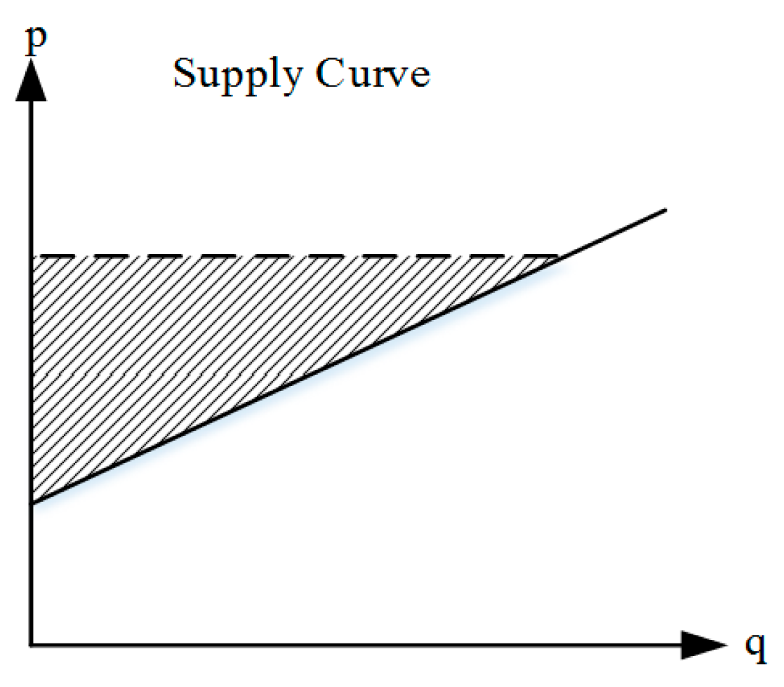
Appendix B
For the producer surplus maximization model:
Figure A1.
Supply curve.

This diagram is just a brief sketch. Regardless of whether the supply curve is linear or nonlinear, the total quantity supplied is a function of the price. The gray shaded area represents producer surplus.
For the consumer surplus maximization model:
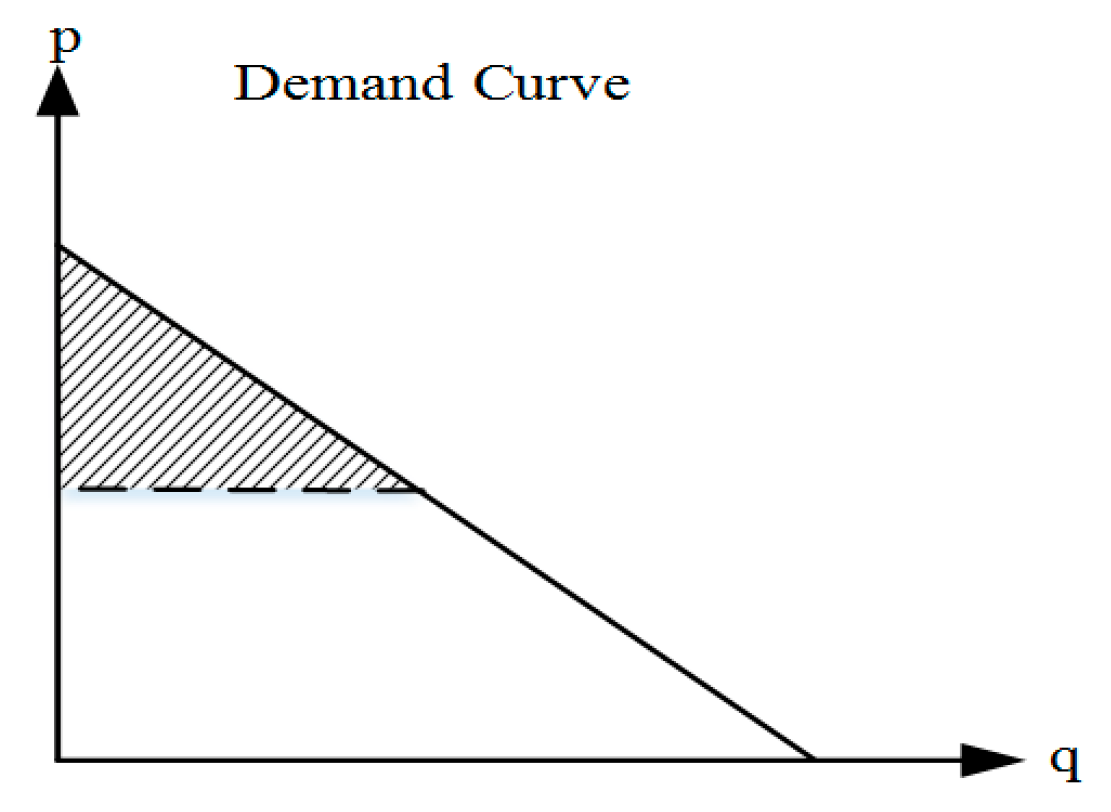
Figure A2.
Demand curve.

This diagram is also just a brief sketch. Regardless of whether the demand curve is linear or nonlinear, the total quantity demanded is also a function of the price. The gray shaded area represents a consumer surplus.
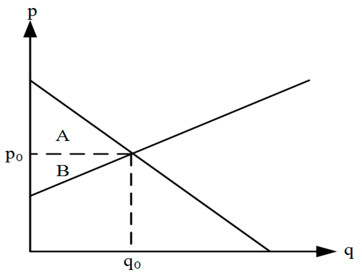
At first sight, each seems to try to optimize its own profit (for firms) or wellbeing (for consumers, usually called utility). However, a market acts as if it maximizes a single objective function, i.e., social welfare [37]. There is a concept of optimality, due to the economist Vilfredo Pareto, that can be applied to economic situations (e.g., production decisions, consumption decisions, and the prices at which things trade) with many different agents: Pareto optimality, also known as Pareto efficiency. Although each producer tries to pursue the maximization of its own interests, these interests (producer surplus) closely relate to the market price (this can be seen in Formula (6)), which is determined by consumers and producers together. Therefore, in the energy market, it is not scientific to choose the energy-consumption strategy through only the producer surplus maximization model. Producers are placed in the market, so their optimal choices are limited by the consumers and the market, which is also the best choice that producers can achieve in the game with consumers. For the social welfare maximization model:
Figure A3.
Social welfare maximization.

This diagram is just a brief sketch. is the equilibrium in the market. A is consumers’ surplus and B is producers’ surplus. At this point, social welfare is maximized.
We want to explore the emission indexes and emissions of enterprises with different energy consumption levels in the market. According to what we have analyzed, solving these problems by only a producer surplus model is not scientific. We should put them in the whole market to solve, following Gabriel et al. [37]. We begin by giving the producer surplus and consumer surplus formulas, then according to the model that Gabriel et al. [37] have mentioned in their book (i.e., in which social welfare maximization is the sum of producer surplus and consumer surplus), we derive the social welfare maximization model to calculate and compare the emission levels of different energy-consumption enterprises in the market, this result is more realistic. So our final model which is used to calculate and compare the emission levels of different energy-consumption enterprises is the social welfare maximization model (Formulas (21)–(28)).
Appendix C
According to Formula (4), when the carbon emission index of company i is smaller than , its carbon tax rate is r1. When the carbon emission index of company i is larger than , its carbon tax rate is r2. is similar. We assume that A is a high energy-consumption company, B is a medium energy-consumption company, and C is a low energy-consumption company. Therefore, should be satisfied (, , and respectively represent carbon emission index of company A, B and C). For , we know that . Combined with the values in Table 1 and Table 2, we calculated by adjusting the proportion of three fuels used that ranges from 0.5 to 0.6 (We keep only one decimal point). Similarly, we found that ranges from 0.3 to 0.4, and
ranges from 0.2 to 0.3. Thus, if is is satisfied, and should be satisfied. Therefore, we set and .
We set in the paper when the price is 0, the market demand is 10,000. According to the inverse demand function , we can get , that is, . We assume when the market is in equilibrium, the price is 188 and the market demand is 5000. Then, when we put the equilibrium (p = 188, qd = 5000) into the inverse demand curve, we can get and . To be clear, the equilibrium (p = 188, qd = 5000) is what we set. Of course other values could also be taken, but would not affect the final relationship of the individual [37].
Just as Gabriel et al. [37] pointed out, the social welfare maximization model and the small-world network model are universal for the traditional manufacturing industries related to carbon emissions (because different parameters can be used to simulate different industries).
References
- Stavins, R.N. The problem of the commons: Still unsettled after 100 years. Am. Econ. Rev. 2011, 101, 81–108. [Google Scholar] [CrossRef]
- Bjorkegren, A.B.; Grimmond, C.S.B.; Kotthaus, S.; Malamud, B.D. CO2 emission estimation in the urban environment: Measurement of the CO2 storage term. Atmos. Environ. 2015, 122, 775–790. [Google Scholar] [CrossRef]
- Milliman, S.R.; Prince, R. Firm incentives to promote technological change in pollution control. J. Environ. Econ. Manag. 1989, 17, 247–265. [Google Scholar] [CrossRef]
- Montgomery, W.D. Markets in licenses and efficient pollution control programs. J. Econ. Theory 1972, 5, 395–418. [Google Scholar] [CrossRef]
- Tietenberg, T.H. Economic instruments for environmental regulation. Oxf. Rev. Econ. Policy 1990, 6, 17–33. [Google Scholar] [CrossRef]
- Agee, M.D.; Atkinson, S.E.; Crocker, T.D.; Williams, J.W. Non-separable pollution control: Implications for a CO2 emissions cap and trade system. Resour. Energy Econ. 2014, 36, 64–82. [Google Scholar] [CrossRef]
- Stavins, R.N. Market-based environmental policies: What can we learn from U.S. Experience (and related research)? Resour. Future 2003, 3–43. [Google Scholar] [CrossRef]
- Nordhaus, W.D. After Kyoto: Alternative mechanisms to control global warming. Am. Econ. Rev. 2005, 96, 31–34. [Google Scholar] [CrossRef]
- Wittneben, B.B.F. Exxon is right: Let us re-examine our choice for a cap-and-trade system over a carbon tax. Energy Policy 2009, 37, 2462–2464. [Google Scholar] [CrossRef]
- Herzog, T.; Baumert, K.A.; Pershing, J. Target: Intensity. An Analysis of Greenhouse Gas Intensity Targets, 1st ed.; World Resources Institute: Washington, DC, USA, 2006; pp. 15–24. ISBN 1-56973-638-3. [Google Scholar]
- Carayol, N.; Roux, P. Knowledge flows and the geography of networks: A strategic model of small world formation. J. Econ. Behav. Organ. 2009, 71, 414–427. [Google Scholar] [CrossRef]
- Hsu, C.-I.; Shih, H.-H. Small-world network theory in the study of network connectivity and efficiency of complementary international airline alliances. J. Air Transp. Manag. 2008, 14, 123–129. [Google Scholar] [CrossRef]
- Sheng, J. Effect of uncertainties in estimated carbon reduction from deforestation and forest degradation on required incentive payments in developing countries. Sustainability 2017, 9, 1608. [Google Scholar] [CrossRef]
- Liu, B.; Li, T.; Tsai, S. Low carbon strategy analysis of competing supply chains with different power structures. Sustainability 2017, 9, 835. [Google Scholar] [CrossRef]
- Li, W.; Li, G.; Zhang, R.; Sun, W.; Wu, W.; Jin, B.; Cui, P. Carbon reduction potential of resource-dependent regions based on simulated annealing programming algorithm. Sustainability 2017, 9, 1161. [Google Scholar] [CrossRef]
- Martin, R.; Muuls, M.; Wagner, U.J. The impact of the European Union emissions trading scheme on regulated firms: What is the evidence after ten years? Rev. Environ. Econ. Policy 2016, 10, 129–148. [Google Scholar] [CrossRef]
- Oestreich, A.M.; Tsiakas, I. Carbon emissions and stock returns: Evidence from the EU emissions trading scheme. J. Bank. Financ. 2015, 58, 294–308. [Google Scholar] [CrossRef]
- Zhang, K.; Wang, Q.; Liang, Q.-M.; Chen, H. A bibliometric analysis of research on carbon tax from 1989 to 2014. Renew. Sustain. Energy Rev. 2016, 58, 297–310. [Google Scholar] [CrossRef]
- Jaeger, W.K. Carbon taxation when climate affects productivity. Land Econ. 2002, 78, 354–367. [Google Scholar] [CrossRef]
- Bruvoll, A.; Larsen, B.M. Greenhouse gas emissions in Norway: Do carbon taxes work? Energy Policy 2004, 32, 493–505. [Google Scholar] [CrossRef]
- Floros, N.; Vlachou, A. Energy demand and energy-related CO2 emissions in Greek manufacturing: Assessing the impact of a carbon tax. Energy Econ. 2005, 27, 387–413. [Google Scholar] [CrossRef]
- Callan, T.; Lyons, S.; Scott, S.; Tol, R.S.J.; Verde, S. The distributional implications of a carbon tax in Ireland. Energy Policy 2009, 37, 407–412. [Google Scholar] [CrossRef]
- Bureau, B. Distributional effects of a carbon tax on car fuels in France. Energy Econ. 2011, 33, 121–130. [Google Scholar] [CrossRef] [Green Version]
- Wesseh, J.P.K.; Lin, B. Optimal emission taxes for full internalization of environmental externalities. J. Clean. Prod. 2016, 137, 871–877. [Google Scholar] [CrossRef]
- Liu, X.; Wang, C.; Niu, D.; Suk, S.; Bao, C. An analysis of company choice preference to carbon tax policy in china. J. Clean. Prod. 2015, 103, 393–400. [Google Scholar] [CrossRef]
- Yates, R. Universal health coverage: Progressive taxes are key. Lancet 2015, 386, 227–229. [Google Scholar] [CrossRef]
- Chiroleu-Assouline, M.; Fodha, M. From regressive pollution taxes to progressive environmental tax reforms. Eur. Econ. Rev. 2014, 69, 126–142. [Google Scholar] [CrossRef]
- Orsi, F. Environment: Progressive taxes for sustainability. Nature 2017, 541, 464. [Google Scholar] [CrossRef] [PubMed]
- Maynard Smith, J. The theory of games and the evolution of animal conflicts. J. Theor. Biol. 1974, 47, 209–221. [Google Scholar] [CrossRef]
- Smith, J.M.; Price, G.R. The logic of animal conflict. Nature 1973, 246, 15–18. [Google Scholar] [CrossRef]
- Taylor, P.D.; Jonker, L.B. Evolutionary stable strategies and game dynamics. Math. Biosci. 1978, 40, 145–156. [Google Scholar] [CrossRef]
- Ji, P.; Ma, X.; Li, G. Developing green purchasing relationships for the manufacturing industry: An evolutionary game theory perspective. Int. J. Prod. Econ. 2015, 166, 155–162. [Google Scholar] [CrossRef]
- Scrimgeour, F.; Oxley, L.; Fatai, K. Reducing carbon emissions? The relative effectiveness of different types of environmental tax: The case of New Zealand. Environ. Model. Softw. 2005, 20, 1439–1448. [Google Scholar] [CrossRef]
- Telli, Ç.; Voyvoda, E.; Yeldan, E. Economics of environmental policy in turkey: A general equilibrium investigation of the economic evaluation of sectoral emission reduction policies for climate change. J. Policy Model. 2008, 30, 321–340. [Google Scholar] [CrossRef] [Green Version]
- Timilsina, G.R.; Shrestha, R.M. General equilibrium effects of a supply side GHG mitigation option under the clean development mechanism. J. Environ. Manag. 2006, 80, 327–341. [Google Scholar] [CrossRef] [PubMed]
- Baron, D.P.; Meyerson, R.B. Regulating a monopolist with unknown costs. Econometrica 1982, 50, 911–930. [Google Scholar] [CrossRef]
- Gabriel, S.A.; Conejo, A.J.; Fuller, J.D.; Hobbs, B.F.; Ruiz, C. Complementarity Modeling in Energy Markets, 1st ed.; Springer: New York, NY, USA, 2013; pp. 72–476. ISBN 978-1-4419-6122-8. [Google Scholar]
- Ho, T.H.; Wang, X.; Camerer, C.F. Individual differences in EWA learning with partial payoff information. Econ. J. 2008, 118, 37–59. [Google Scholar] [CrossRef]
- Xian, Y.B.; Mei, L. Adaptive expectation, complex network and the dynamic of standard diffusion—Research based on computational economics. J. Manag. Sci. 2007, 20, 62–71. [Google Scholar] [CrossRef]
- Watts, D.J.; Strogatz, S.H. Collective dynamics of ‘small-world’ networks. Nature 1998, 393, 440–442. [Google Scholar] [CrossRef] [PubMed]
- Newman, M.E.J.; Watts, D.J. Renormalization group analysis of the small-world network model. Phys. Lett. A 1999, 263, 341–346. [Google Scholar] [CrossRef]
Figure 1.
Changes in the emission index and emissions of enterprises with high energy consumption. (a) The change of emission index of enterprises with high energy consumption. (b) The change of emission of enterprises with high energy consumption.
Figure 1.
Changes in the emission index and emissions of enterprises with high energy consumption. (a) The change of emission index of enterprises with high energy consumption. (b) The change of emission of enterprises with high energy consumption.

Figure 2.
Changes in the emission index and emissions of enterprises with medium energy consumption. (a) The change of emission index of enterprises with medium energy consumption. (b) The change of emission of enterprises with medium energy consumption.
Figure 2.
Changes in the emission index and emissions of enterprises with medium energy consumption. (a) The change of emission index of enterprises with medium energy consumption. (b) The change of emission of enterprises with medium energy consumption.

Figure 3.
Changes in the emission index and emissions of enterprises with low energy consumption. (a) The change of emission index of enterprises with low energy consumption. (b) The change of emission of enterprises with low energy consumption.
Figure 3.
Changes in the emission index and emissions of enterprises with low energy consumption. (a) The change of emission index of enterprises with low energy consumption. (b) The change of emission of enterprises with low energy consumption.
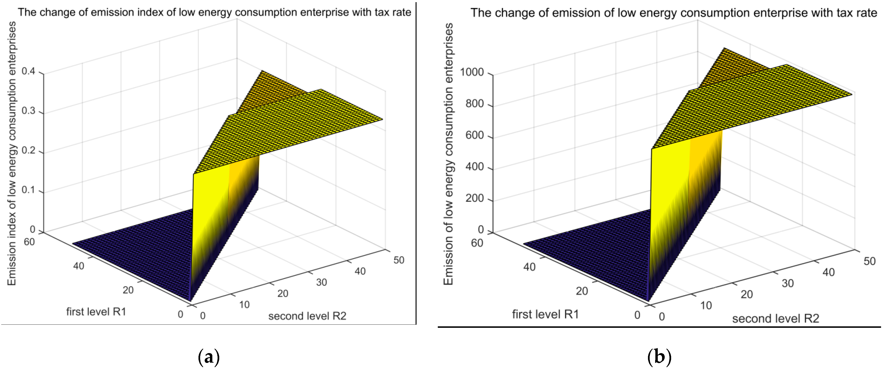
Figure 4.
Evolution of the number of enterprises adopting the three energy consumption strategies under standard parameters.
Figure 4.
Evolution of the number of enterprises adopting the three energy consumption strategies under standard parameters.

Figure 5.
Evolutionary result when the discount coefficient of enterprises δ = 0.1.

Figure 6.
Evolutionary result when the discount coefficient of enterprises δ = 0.9.

Figure 7.
Evolutionary result when the price of the low energy consumption strategy is .

Figure 8.
Evolutionary result when the price of the low energy consumption strategy is .

Figure 9.
Evolutionary result when the network effect parameter .

Figure 10.
Evolutionary result when the network effect parameter .

Figure 11.
Evolutionary result when the expected adjustment factor ξ = 0.1.
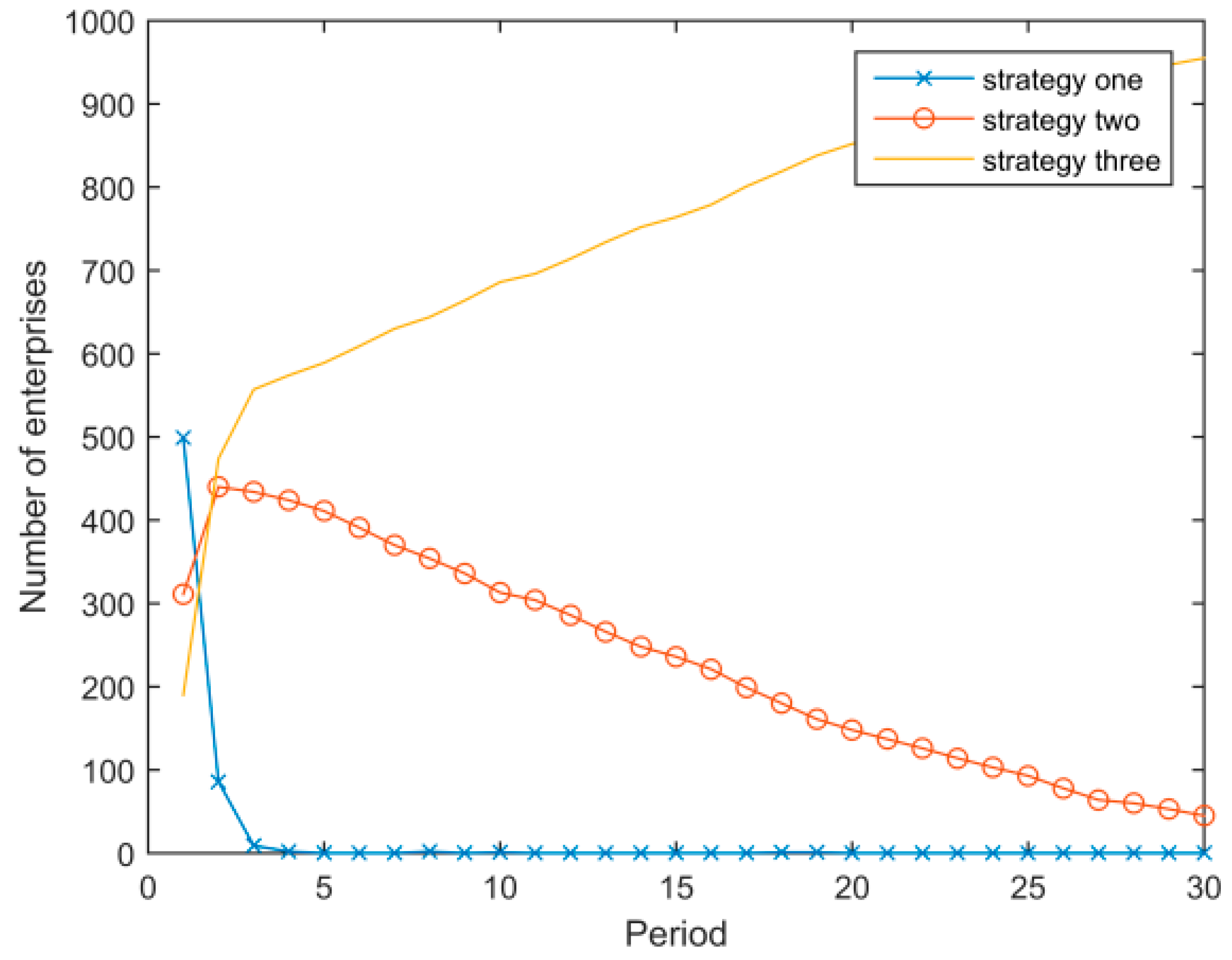
Figure 12.
Evolutionary result when the expected adjustment factor ξ = 0.9.


Table 1.
Fuel parameters.
| Type of Fuel | Variable Cost (VC) | Energy | Emission Factor |
|---|---|---|---|
| wil | hl (US $/t 100 m3) | (GJ/t·100 m3) | el (t CO2/t·100 m3) |
| coal | 100 | 32.1 | 2.457 |
| petroleum coke | 50 | 23.3 | 2.53 |
| natural gas | 11 | 3.72 | 0.29 |
Table 2.
Enterprise parameters.
| Enterprise | Cost of Production | Limit of Production Capacity | Energy | ||
|---|---|---|---|---|---|
| ci ($/t) | ti | di | bi (GJ/t) | ||
| A | 22 | 0.001 | 3000 | 6 | |
| B | 26 | 0.001 | 3000 | 4.5 | |
| C | 29 | 0.001 | 3000 | 3 | |
Table 3.
Carbon emissions and income statements for three enterprises with different levels of energy consumption.
Table 3.
Carbon emissions and income statements for three enterprises with different levels of energy consumption.
| Emission Index | Emissions | Environmental Cost | Pre-Tax Profit | After-Tax Profit | |
|---|---|---|---|---|---|
| High energy consumption enterprise | 0.4677 | 1253.6 | 12,138 | 19,320.5 | 7182.5 |
| Medium energy consumption enterprise | 0.3508 | 1052.4 | 4115.3 | 33,973.3 | 29,858 |
| Low energy consumption enterprise | 0.3000 | 900 | 0 | 52,534 | 52,534 |
© 2017 by the authors. Licensee MDPI, Basel, Switzerland. This article is an open access article distributed under the terms and conditions of the Creative Commons Attribution (CC BY) license (http://creativecommons.org/licenses/by/4.0/).
Share and Cite
MDPI and ACS Style
Wu, B.; Huang, W.; Liu, P. Carbon Reduction Strategies Based on an NW Small-World Network with a Progressive Carbon Tax. Sustainability 2017, 9, 1747. https://doi.org/10.3390/su9101747
AMA Style
Wu B, Huang W, Liu P. Carbon Reduction Strategies Based on an NW Small-World Network with a Progressive Carbon Tax. Sustainability. 2017; 9(10):1747. https://doi.org/10.3390/su9101747
Chicago/Turabian StyleWu, Bin, Wanying Huang, and Pengfei Liu. 2017. "Carbon Reduction Strategies Based on an NW Small-World Network with a Progressive Carbon Tax" Sustainability 9, no. 10: 1747. https://doi.org/10.3390/su9101747
Note that from the first issue of 2016, this journal uses article numbers instead of page numbers. See further details here.