An Analysis of Decision Factors on the Price of South Korea’s Certified Emission Reductions in Use of Vector Error Correction Model


Department of Energy Resources Engineering, Inha University, 100 Inharo, Nam-gu, Incheon 22212, Korea
*
Author to whom correspondence should be addressed.
Sustainability 2017, 9(10), 1768; https://doi.org/10.3390/su9101768
Submission received: 16 August 2017
/
Revised: 25 September 2017
/
Accepted: 27 September 2017
/
Published: 29 September 2017
(This article belongs to the Section Economic and Business Aspects of Sustainability)
Abstract
:This study analyzes factors affecting the price of South Korea’s Certified Emission Reduction (CER) using statistical methods. CER refers to the transaction price for the amount of carbon emitted. Analysis of results found a co-integration relationship among the price of South Korea’s CER, oil price (WTI), and South Korea’s maximum electric power demand, which means that there is a long-term relationship among the three variables. Based on this result, VECM (vector error correction model) analysis, impulse response function, and variance decomposition were performed. As the oil price (WTI) increases, the demand for gas in power generation in Korea declines while the demand for coal increases. This leads to increased greenhouse gas (GHG; e.g., CO2) emissions and increased price of South Korea’s CERs. In addition, rising oil prices (WTI) cause a decline in demand for oil products such as kerosene, which results in an increase in South Korea’s maximum power demand.
1. Introduction
Erratic weather phenomena caused by climate change threatens the survival of mankind. According to UN reports on climate change, environmental disasters caused by climate change can cause unexpected serious problems. In addition, climate change can cause economic, social, as well as environmental problems [1,2,3,4,5]. The increase in GHGs (greenhouse gases) is a major cause of global warming. In order to address global warming, climate change agreements such as the Kyoto Protocol have been reached concerning GHG emissions [6,7,8,9,10]. In Korea, energy services are variously explored [11,12,13,14] and related renewable energy policy is in action [15,16,17,18,19,20]. The Korean government is making an effort to enhance the efficiency of electricity generation [21]. According to Marques et al. [22], power generation using conventional fossil resources has shown a positive causal relationship to Greek economic growth in the short term. However, the causal relationship between power generation and economic growth using renewable electricity was not clear. In addition, Greece’s economic growth is considered to be short-term causes of electricity generation using renewable electricity. However, there was no causal relationship in the reverse. The Certified Emission Reduction (CER) is the GHG reduction system as set out in Article 17 of the Kyoto Protocol, which establishes the transaction price for the amount of carbon emitted. It allows governments to allocate annual emission credits to companies emitting GHG. This is a system that permits business-to-business transactions involving emission credits. South Korea’s emissions trading system has been in effect from 1 January 2015, in accordance with Article 46 of the “Low Carbon, Green Growth”, and has been listed on the Korea Exchange.
There have been studies regarding the factors affecting the price of the EU’s CER. Mansanet-Battaller et al. [23] used the ratio of fossil energy price and power price as variables. The coefficient of energy prices was found not statistically significant at the 1% level. The coefficient of electricity price was statistically significant at the 5% level. The time-lagged Brent oil price and the coefficient of electricity price were statistically significant at the 1% level. In addition, the price of CER increased as energy prices increased. This supports the assumption that as the price of oil and gas used for power rises, the demand for coal as an alternative fuel source increases, which results in an increase in carbon emissions. Subsequently, the increase in carbon emissions causes an increase in demand for carbon credits and an increase in the price of the CER. However, it is assumed that there is a coupling relationship between the price of oil and gas.
Kim [16] analyzed the correlation between the price of the EU’s CER and the price of energy utilizing daily and weekly data. Concerning the daily data analysis, the correlation between the price of the EU’s CER and oil price was high, and the price difference between coal and gas was not statistically significant. In addition, the relationship between electricity price and emission price was not statistically significant. Regarding the weekly data analysis, the price of the EU’s CER was highly correlated with oil price. However, electricity price was not statistically significant in correlation with emission price. As a result, it was concluded that the volatility of oil prices could predict the volatility in price of the EU’s CER.
Conversely, Park [24] used a linear regression model to define the price volatility of South Korea’s CER. The closing price data of the KAU15 (Korea Allowance Unit) and the KCU15 (Korea Credit Unit) were used for the price of South Korea’s CER. KAU 15 data was obtained from 12 January 2015–30 June 2015, and KCU 15 data included the period from 6 April 2015–30 June 2016. The explanatory variables included energy price, temperature index, and economic outlook index.
It was found that the energy variables (oil and electricity) were not statistically significant in both cases. Park [24] proposed that the government separately imposed the settlement of emission trading costs because the price of emission credits was not reflected in the price of electricity. The temperature index and the cooling index—which are associated with energy—were not affected by the price of South Korea’s CER. Park [24] found that statistically valid pricing factors in prior studies are not valid for South Korea’s CER market.
Based on theoretical principles and research experience, we conducted a time series analysis using VECM (vector error correction model) with oil price (WTI) and maximum power demand in South Korea to determine whether South Korea’s CER is consistent with findings in previous studies. South Korea’s emissions trading system has been in effect since 1 January 2015. However, the transaction volume has been small and has been evaluated as a nominal market. Additionally, there is the limitation that the data for time series analysis is extremely short. However, it is meaningful to conduct the time series analysis of South Korea’s CER, which has not been tested using time series analysis with oil price (WTI) and South Korea’s maximum power demand prior.
2. Materials and Methodology
South Korea’s CER has been listed on the Korean exchange market since 2015. South Korea’s CER can be divided into the KAU (Korean Allowance Unit), the KCU (Korean Credit Unit), and the KOC (Korea Offset Credit). The KAU is the allowable amount of GHG emission allocated to companies. At the beginning of each planning period, it is listed by classifying the transactions. The KCU is the emission rights converted from external business GHG reductions by specific implementation year, and the listing period is not specified and is flexible. The KOC is the government’s allowance of GHG emissions that the business owners have reduced out of the businesses where they are assigned. There are different types of CERs, including the KAU 16, KAU 17, KCU 16, and KCU 17. However, it has not been long that a sufficient volume of transactions has occurred. The transaction volume has increased since 16 June. This is because companies felt the need to deal with emissions trading as they go through the implementation year of carbon emission rights.
Meanwhile, there is no sufficient volume of transactions except for the KAU 16. Therefore, the KAU 16 was chosen as the study data for South Korea’s CER. We collected the weekly price of South Korea’s CER from the Korean exchange market from 13 June 2016 to 22 May 2017 as well as the oil price (WTI) from the NYMEX, and South Korea’s maximum power demand from Korean Power Exchange as data for analysis (Table 1).
This study conducted unit root tests for the price of South Korea’s CER (EMI), oil price (OIL), and South Korea’s maximum power demand (ELEC). In the case that these tests found evidence of I(1) (integrated of order one), the co-integration test was used to determine co-integration employing prior research methods. Finally, the VECM (vector error correction model) was applied according to test results [25,26,27,28].
Regarding the VECM analysis, the stability of the time series was verified through the unit root test, and then the long-term relationship was examined through the co-integration test. Finally, estimation of the short- and long-term causal relationship was conducted using the VECM. This is because VECM uses raw data rather than first-order data, so it is possible to estimate the long-term causation as well as short-term causal relationships that can be identified by a general Granger test [29,30,31].
Prior to conducting the time series methods, we must consider whether each dataset has a unit root. Unit root makes the result invalid if they are not accounted for. However, in the analysis of co-integration using the VECM, although each dataset has a unit root, they can be accounted for through the co-integration test [32,33,34,35].
There are various stationary tests for testing the unit root. The augmented Dickey–Fuller test and the Phillips and Perron test were used in this study because the insufficient data may produce untrustworthy results using only one test.
If it is concluded that there is a unit root in the data, then the co-integration test can be applied. The co-integration test is used to confirm the existence of a linear combination integrated of order zero.
A non-stationary time series which has unit roots and linear combination I(0) is called a co-integration relation. The existence of co-integration means that if one variable is broken with another variable in a co-integration relation, this state does not persist for long before returning to the previous stable relationship. Therefore, there is a long-run equilibrium relation between variables [29,30].
While there are various co-integration tests, the Johansen co-integration test is used in this study.
If the co-integration relation is confirmed by way of the co-integration test, the short- and long-term causality can be tested through the VECM as follows.
Consider the equations below. represent the long-term causality. Therefore, if they are meaningful, it can be concluded that long-term causality statistically exists for the data. These terms are for short-term causality. So, if they are meaningful, it can be concluded that short-term causality statistically exists for the data.
In addition to the VECM analysis, we will show the meaningful methods used to analyze our data. Impulse responses are required to understand results in the short term. The impulse response function is a moving average model which shows how the variables in the model respond to shocks over time, given the unexpected economic impacts. There is also the advantage that it is easy to check conveniently through the graph. Finally, it is straightforward to grasp causal relationships between the variables and to analyze the influence of variables [27,28,29,30].
Variance decomposition is also used to enhance the interpretation of results in the short term. Variance decomposition is a method of describing the relational characteristics of variables with impulse response analysis. The prediction error of a specific variable includes several impact factors of other variables. The method of decomposing these factors is variance decomposition. In other words, it is possible to analyze the relative importance of the endogenous variables in the error terms of the vector autoregressive model through variance decomposition [27,30].
3. Results and Discussion
The results of the unit root tests show that in the case of the inclusion of trends, the null hypothesis that the unit root exists at a significance level of 5% cannot be rejected for the price of South Korea’s CER and South Korea’s maximum power demand. However, the augmented Dickey–Fuller (ADF) and Phillips and Perron (PP) tests for the first difference show they have no unit root at the 5% significance level, indicating that both the price of South Korea’s CER and South Korea’s maximum power demand are I(1). In other words, each variable in the unstable time series is stabilized when the first difference is applied.
Conversely, the results of the unit root test for the price of oil differ. Therefore, careful judgment is required. Regarding the price of oil’s unit root test, the null hypothesis is rejected at the 5% significance level. This means that the price of oil does not have a unit root at the 5% significance level. This is suspicious, because generally it is known that the price of oil has a unit root. This unexpected result may be due to insufficient data. In the case of the Phillips and Perron test, it has a unit root. We accepted the Phillips and Perron test (Table 2).
Since all variables are I(1), the co-integration test can be conducted to determine whether there is a stable co-integration relation between variables. The Johansen co-integration test was used in this study, and the optimal lag length was determined according to the results of the AIC and SIC analyses.
It is shown that each dataset has a unit root. Therefore, we can apply the co-integration test to determine whether the linear combination is stationary.
According to the maximum value, it is rejected that it has no co-integration relationship, and it is not rejected that it has at most 1 and 2 co-integration relationships at the 5% significance level. In short, this means that the linear combination has one co-integration relationship. However, when it comes to the trace value, there is no co-integration relationship at the 5% significance level. This is contrary to the result for the maximum value. In this case, Johansen stated that we can base our choice on the interpretability of the co-integrating relations. This study chose the maximum value. Therefore, there is a long-term equilibrium relation between variables (Table 3 and Table 4).
The trace statistic and the maximum eigenvalue statistic may yield conflicting results. For such cases, we recommend that you examine the estimated co-integrating vector and base your choice on the interpretability of the co-integrating relations; see Johansen [30] for an example.
According to this result, VECM was performed. The optimal lag length was determined according to the results of the AIC and SC analyses. The results of VECM found the ECT coefficient of the price of South Korea’s CER was −0.14, statistically significant at 1% with an absolute value of t above 3.0. This means that there is a long-term causal relationship between the price of oil and South Korea’s maximum power demand with the price of South Korea’s CER. In addition, this means that deviating part in the previous period will be recovered to this period from the long-term relationship. This is consistent with previous research concerning the price of the EU’s CER.
On the other hand, the estimation results show the short-term coefficients , , and indicate a short-term causal relationship. The differenced data of the price of South Korea’s CER is 0.636013 and −0.149786. The shock in the previous period led to a rise in the current period, and the shock in the period before the previous period led to a fall in this period.
The differenced data of the price of oil is 60.10426 and −160.7532. The shock in the previous period led to a rise in the current period and the shock in two periods prior led to a fall in the current period. However, the standard error is too high to trust.
The differenced data of South Korea’s maximum power demand is −0.041627 and 0.005906. The shock in the previous period led to a fall in the current period and the shock in two periods prior led to a rise in the current period (Table 5).
Regarding the impulse response function, the first graph indicates the response of the price of South Korea’s CER to the price of oil’s one standard deviation. The price of South Korea’s CER increased for 7 weeks following a shock in the price of oil.
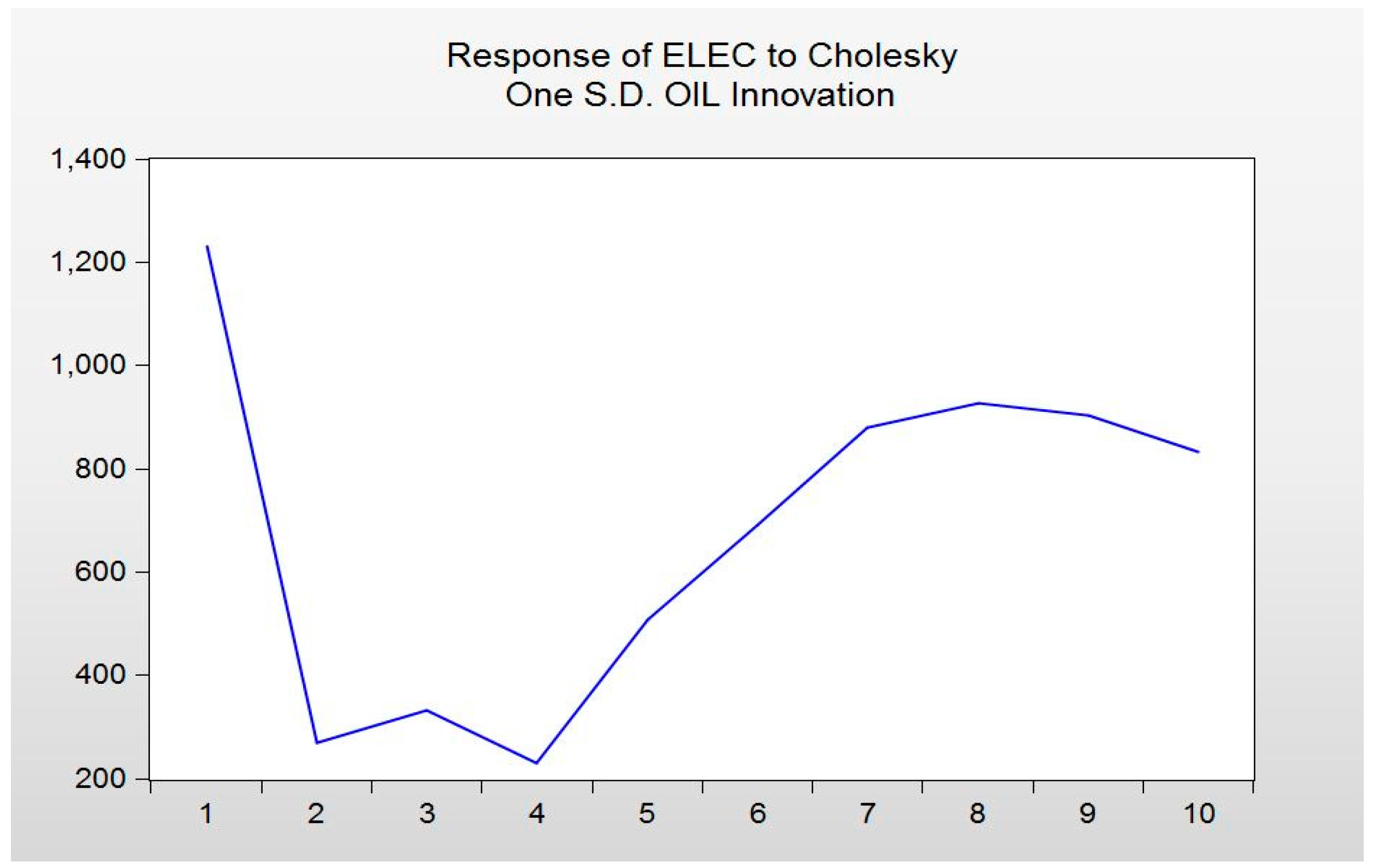
The second graph indicates the response of South Korea’s maximum power demand to the price of oil’s one standard deviation. Initially, it decreased for about 2 weeks, but subsequently increased after 4 weeks. These results confirm previous research.
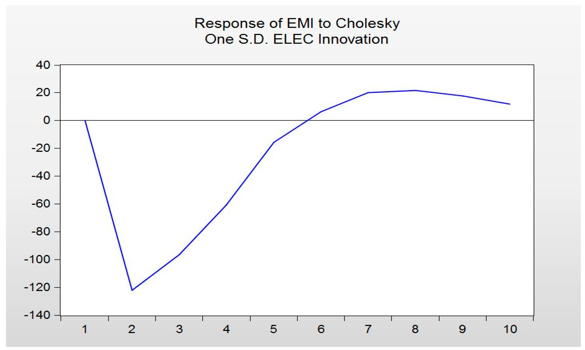
However, the last graph indicates the response of the price of South Korea’s CER to South Korea’s maximum power demand is in contrast to previous studies. Insufficient and uncertainty in data—especially in the price of South Korea’s CER—may have produced these unreliable results (Figure 1, Figure 2 and Figure 3).
Korea’s CER was performed. The variance of the forecast error for South Korea’s CER is explained by 86.1% by self in early stage (t = 3), the price of oil (12.3%), and the maximum power demand of (1.5%). Following the 10th period (t = 10), the variance is explained by 56% by self, 43.7% by the price of oil, and 0.34% by the maximum power demand in South Korea. It can be concluded that the price of South Korea’s CER is heavily influenced by the price of oil. This is consistent with previous studies that found the price of oil has a significant effect on the CER. However, the standard error was high (Table 6).
4. Conclusions
This study conducted time series analysis by employing the VECM (vector error correction model). We assessed oil price (WTI) and maximum power demand in South Korea using data from 13 June 2016–22 May 2017 to determine whether South Korea’s CER is consistent with previous studies. Since all variables were I(1), the Johansen co-integration test was employed to determine whether there was a stable co-integration relation between variables. The linear combination composed of each variable had one co-integration relationship. Therefore, there was a long-term equilibrium relation between variables. Results of VECM found the ECT coefficient of the price of South Korea’s CER was −0.14 and statistically significant at 1%, with an absolute value of t above 3.0.
There was a long-term causal relationship in the price of oil and South Korea’s maximum power demand with the price of South Korea’s CER. Therefore, it can be concluded that deviating part in the previous period will be recovered to this period from the long-term relationship. Conversely, the estimation results showed some statistically significant coefficients in the short-term relationship between variables. Concerning the impulse response function, as time passed, the response of the price of South Korea’s CER increased by the price of oil’s one standard deviation. In addition, the response of South Korea’s maximum power demand decreased for approximately 2 weeks, and subsequently increased after 4 weeks by the price of oil’s one standard deviation. However, the response of the price of South Korea’s CER to South Korea’s maximum power demand was contrary to the theory.
Oil price is closely related to the price of gas, as electric power companies will decrease the demand for gas and increase the demand for coal in the case of higher price of oil. This leads to increasing CO2 emissions. In the long term, the price of South Korea’s CER will increase. In other words, as the oil price (WTI) rises, the demand for gas for power generation in South Korea decreases while the demand for coal increases. This results in an increase in GHG emissions and a rise in the price of South Korea’s CER. In addition, if the price of oil increases, the demand for oil products such as kerosene decrease and subsequently, demand for electricity increases. Eventually, maximum power demand increases.
Most results were consistent with previous studies. However, there were exceptions. First, we did not obtain sufficient data for time series analysis. In particular, South Korea’s CER transaction volume was limited in that it has been evaluated as a nominal market. Additionally, a limitation to this study is that the data used for time series analysis was limited.
In Marques et al. [22], there were no major driving energy sources of economic growth in Greece. Except for conventional fossil sources, energy sources have a limited impact on the industrial production index (IPI). From these results, Marques et al. [22] concluded that disturbance in economic activity has a greater impact on fossil-based power generation than renewable.
However, it is meaningful to conduct time series analysis of South Korea’s CER, which has not been attempted previously involving oil price (WTI) and South Korea’s maximum power demand. The volume of trading and price was controlled and restricted by government. These factors can have adverse effects on analysis results involving time series data.
The Korean government can use this result in the CERs policy making [36]. CERs’ prices are closely related to oil price (WTI) and South Korea’s maximum electric power demand. Therefore, the Korean government can approximately forecast price volatility and trade volume of CERs in the future. As a result, the Korean government can assign the volume of the reduction target more scientifically.
In South Korea, certified emission reductions have been traded for one and half years. They are very new data. Therefore, this paper can use only those periods of CERs data. Though the data has some weakness in length, the data are a very new and original contribution of this research. The authors can suggest future research in the use of longer series of Korea’s CERs data after three or four years.
Acknowledgments
This paper has been funded by National Research Foundation-2016R1A2B1014142, National Research Foundation-NRF-2015-S1A3A-2046742 (SSK), and Inha university.
Author Contributions
Park and Lee conceived and designed the experiments; Park and Lee performed the experiments; Park and Lee analyzed the data; Park and Lee contributed reagents/materials/analysis tools; Park and Lee wrote the paper.
Conflicts of Interest
The authors declare no conflict of interest.
References
- Gi-duck, B. The Determination of Carbon Price and Interaction of Carbon and Electricity Prices; Department of Economics, Graduate School, Kyungbook National University: Daegu, Korea, 2011. [Google Scholar]
- Chae, J.O.; Sun-Kyoung, P. Status of Korea ETS and Strategies to improve in One Year After Launching—Through Comparing with EU ETS. J. Clim. Chang. Res. 2016, 7. [Google Scholar] [CrossRef]
- Copeland, B.; Taylor, M. Trade, Growth and the Environment. J. Econ. Lit. 2004, 42, 7–71. [Google Scholar] [CrossRef]
- Dasgupta, S.B.; Laplante, B.; Wang, H.; Wheeler, D. Confronting the Environmental Kuznets Curve. J. Econ. Perspect. 2002, 16, 147–168. [Google Scholar] [CrossRef]
- Holtz-Eakin, D.; Selden, T.M. Stoking the Fires. CO2 Emissions and Economic Growth. J. Public Econ. 1995, 57, 85–101. [Google Scholar] [CrossRef]
- Galeotti, M.; Manera, M.; Lanza, A. On the Robustness of Robustness Checks of the Environmental Kuznets Curve Hypothesis. Environ. Resour. Econ. 2009, 42, 551–574. [Google Scholar] [CrossRef]
- Grossman, G.M.; Krueger, A.B. Environmental Impacts of a North American Free Trade Agreement; NBER Working Paper 3914; National Bureau of Economic Research: Cambridge, MA, USA, 1991. [Google Scholar]
- Le, C.C. Energy Consumption and GDP in Developing Countries: A Co-integrated Panel Analysis. Energy Econ. 2005, 27, 415–427. [Google Scholar] [CrossRef]
- Le, C.C.; Chang, C.P. Energy Consumption and GDP Revisited: A Panel Analysis of Developed and Developing Countries. Energy Econ. 2007, 29, 1206–1223. [Google Scholar] [CrossRef]
- Lopez, R. The Environment as a Factor of Production: The Effects of Economic Growth and Trade Liberalization. J. Environ. Econ. Manag. 1994, 27, 163–184. [Google Scholar] [CrossRef]
- Jung, K.-O.; Chung, Y.-K. The Pollution and Economic Growth Based on the Multi-country Comparative Analysis. J. Ind. Econ. Bus. 2004, 17, 1077–1098. [Google Scholar]
- Jung, Y.; Kim, S. Analysis on the Relationship between CO2 Emissions, Economic Growth and Energy Mix. Environ. Resour. Econ. Rev. 2012, 21, 271–297. [Google Scholar]
- Kim, S. Analysis and Forecast of Emission Trading Pricing Factors; Korea Energy Economics Institute: Ulsan, Korea, 2007. [Google Scholar]
- Kim, S. Forecasting Model for Long-Term Energy Demand System; Korea Energy Economics Institute: Ulsan, Korea, 2008. [Google Scholar]
- Huh, S.Y.; Woo, J.; Lim, S.; Lee, Y.G.; Kim, C.S. What do customers want from improved residential electricity services? Evidence from a choice experiment. Energy Policy 2015, 85, 410–420. [Google Scholar] [CrossRef]
- Kim, W. Comparative Analysis on the Determinants of CO2 Emission Per Capita of Main Countries; KIET Monthly Industrial Economics; Korea Institute for Industrial Economics & Trade: Seoul, Korea, 2011; pp. 41–53. [Google Scholar]
- Lim, S.; Huh, S.Y.; Shin, J.; Lee, J.; Lee, Y.G. Enhancing public acceptance of renewable heat obligation policies in South Korea: Consumer preferences and policy implications. Energy Econ. 2017, in press. [Google Scholar] [CrossRef]
- Shin, E. Climate Change; Jip-moon-dang: Seoul, Korea, 2005. [Google Scholar]
- Shin, S.; Hwang, S.; Lee, J.; Kim, S. Long-Term Forecasts of Main Macroeconomic Indicatiors of Korea; Korea Development Institute: Seoul, Korea, 2013. [Google Scholar]
- Shon, H. Study on a change in Japan’s green growth-related policy. Law Res. Inst. Chungbuk Nat. Univ. 2013, 24, 369–396. [Google Scholar]
- Oh, D.H.; Lee, Y.G. Productivity decomposition and economies of scale of Korean fossil-fuel power generation companies: 2001–2012. Energy 2016, 100, 1–9. [Google Scholar] [CrossRef]
- Marques, A.C.; Fuinhas, J.A.; Menegaki, A.N. Interactions between electricity generation sources and economic activity in Greece: A VECM approach. Appl. Energy 2014, 132, 34–46. [Google Scholar] [CrossRef]
- Mansanet-Bataller, M.; Pardo, A.; Valor, E. CO2 prices, energy and weather. Energy J. 2007, 28, 73–92. [Google Scholar] [CrossRef]
- Park, C. A Study on the Analysis of Carbon Trading Market and the Activation Plan in Korea Food and Resource Economics; Korea University: Seoul, Korea, 2017. [Google Scholar]
- Box, G.E.; Jenkins, G.M. Time Series Analysis: Forecasting and Control, Revised ed.; Holden-Day: San Francisco, CA, USA, 1976. [Google Scholar]
- Elliot, G.; Rothenberg, T.; Stock, J. Efficient Tests for an Autoregressive Unit Root. Econometrica 1996, 64, 813–836. [Google Scholar] [CrossRef]
- Engle, R.; Granger, C. Co-integration and Error Correction: Representation, Estimation, and Testing. Econometrica 1987, 55, 251–276. [Google Scholar] [CrossRef]
- Hamilton, J.D. Time Series Analysis; Princeton University Press: Princeton, NJ, USA, 1994; Volume 2. [Google Scholar]
- Hansen, B. Efficient Estimation and Testing of Cointegrating Vectors in the Presense of Deterministic Trends. J. Econom. 1992, 53, 87–121. [Google Scholar] [CrossRef]
- Johansen, S. Estimation and Hypothesis Testing of Cointegration Vectors in Gaussian Vector Autoregressive Models. Econometrica 1991, 59, 1551–1580. [Google Scholar] [CrossRef]
- Kwiatowski, D.; Phillips, P.; Schmidt, P.; Shin, Y. Testing the Null Hypothesis of Stationary against the Alternative of a Unit Root. J. Econom. 1992, 54, 159–178. [Google Scholar] [CrossRef]
- Phillips, P.; Perron, P. Testing for a Unit Root in Time Series Regression. Biometrika 1988, 75, 335–346. [Google Scholar] [CrossRef]
- Phillips, P.; Hansen, B. Statistical Inference in Instrument Variables Regression with I(1) Processes. Rev. Econ. Stud. 1990, 57, 99–125. [Google Scholar] [CrossRef]
- Phillips, P.; Ouliaris, S. Asymptotic Properties of Residual Based Tests for Cointegration. Econometrica 1990, 58, 165–193. [Google Scholar] [CrossRef]
- Hill, R.C.; Griffiths, W.E.; Lim, G.C. Principles of Econometrics, 4th ed.; Wiley: Hoboken, NJ, USA, 2011. [Google Scholar]
- ME, A Study on the Analysis of Carbon Trading Market and the Activation Plan in Korea, Homepage of Ministry of Environment in Korea. 2016. Available online: http://me.go.kr (accessed on 21 July 2017).
Figure 1.
Impulse response of the price of South Korea’s CER to the price of oil’s one standard deviation.
Figure 1.
Impulse response of the price of South Korea’s CER to the price of oil’s one standard deviation.
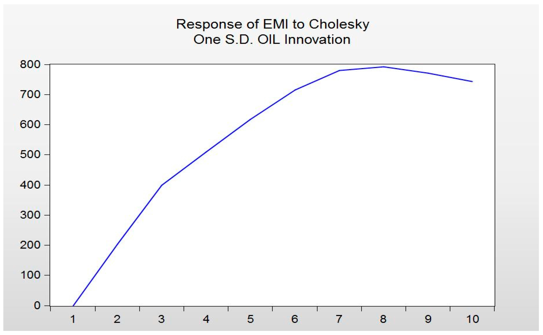
Figure 2.
Impulse response of South Korea’s maximum power demand to the price of oil’s one standard deviation.
Figure 2.
Impulse response of South Korea’s maximum power demand to the price of oil’s one standard deviation.

Figure 3.
Impulse response of the price of South Korea’s CER to the South Korea’s maximum power demand.
Figure 3.
Impulse response of the price of South Korea’s CER to the South Korea’s maximum power demand.


Table 1.
Used data and variables. CER: Certified Emission Reduction.
| Data | Name | Reference |
|---|---|---|
| Price of South Korea’s CER | EMI | Korea exchange |
| Oil price (WTI) | OIL | NYMEX |
| Price of Maximum power demand | ELEC | Korean power exchange |
Table 2.
Unit root test for variables.
| Variables | Methodology | Integration | Prob |
|---|---|---|---|
| EMI | ADF | I(1) | 0.3879 |
| PP | I(1) | 0.5589 | |
| OIL | ADF | I(0) | 0.0486 |
| PP | I(1) | 0.4074 | |
| ELEC | ADF | I(1) | 0.1221 |
| PP | I(1) | 0.1216 |
Notes: Test: H0: Exist a unit root; Critic value: 5 and 1 percent (p = 0.05 dhe p = 0.01) to reject H0. If p > 0.05, we accept H0. Methodology: ADF (augmented Dickey–Fuller), PP (Phillips and Perron). Lags: The number of lags is determined by the information criteria: SIC—Schwartz information criteria.
Table 3.
The estimation of co-integration vectors (trace).
| Unrestricted Co-Integration Rank Test (Trace) | ||||
|---|---|---|---|---|
| Hypothesized No. of CE(s) | Eigenvalue | Trace Statistic | 0.05 Critic Value | Prob. |
| None | 0.367605 | 28.32099 | 29.79707 | 0.0732 |
| At most 1 | 0.079995 | 6.325442 | 15.49471 | 0.6571 |
| At most 2 | 0.047251 | 2.323391 | 3.841466 | 0.1274 |
Notes: Included observations: 48 after adjustment. Trend assumption: Linear deterministic trend. Series: EMI OIL ELEC. Lags interval (in first differences): 1 to 1. Trace test indicates no co-integrating eqn(s) at the 0.05 level.
Table 4.
The estimation of co-integration vectors (maximum eigenvalue).
| Unrestricted Co-integration Rank Test (Maximum Eigenvalue) | ||||
|---|---|---|---|---|
| Hypothesized No. of CE(s) | Eigenvalue | Statistic Max-Eigen | 0.05 Critic value | Prob. |
| None | 0.367605 | 21.99555 | 21.13162 | 0.0377 |
| At most 1 | 0.079995 | 4.002051 | 14.26460 | 0.8591 |
| At most 2 | 0.047251 | 2.323391 | 3.841466 | 0.1274 |
Notes: Max eigenvalue test indicates 1 co-integrating eqn(s) at the 0.05 level.
Table 5.
Error correction model for weekly level of Price of South Korea’s CER (EMI).
| Error Correction | D(EMI) | D(OIL) | D(ELEC) |
|---|---|---|---|
| ECT | −0.147551 | 0.000316 | 0.201911 |
| (0.04805) | (0.00014) | (0.37144) | |
| [−3.07077] | [2.23168] | [0.54359] | |
| D(EMI(−1)) | 0.636013 | 3.64 × 10⁻⁵ | 0.758768 |
| (0.14048) | (0.00041) | (1.08595) | |
| [4.52736] | [0.08811] | [0.69871] | |
| D(EMI(−2)) | −0.149786 | 0.000153 | 0.230365 |
| (0.13855) | (0.00041) | (1.07105) | |
| [−1.08107] | [0.37441] | [0.21508] | |
| D(OIL(−1)) | 60.10426 | 0.680669 | −236.641 |
| (49.0027) | (0.14418) | (378.800) | |
| [1.22655] | [4.72099] | [−0.62483] | |
| D(OIL(−2)) | −160.7532 | −0.221977 | −85.00876 |
| (62.0553) | (0.18258) | (479.699) | |
| [−2.59048] | [−1.21576] | [−0.17721] | |
| D(ELEC(−1)) | −0.041627 | 1.57 × 10⁻⁵ | −0.322728 |
| (0.02289) | (6.7 × 10⁻⁵) | (0.17698) | |
| [−1.81816] | [0.23330] | [−1.82351] | |
| D(ELEC(−2)) | 0.005906 | 2.78 × 10⁻⁵ | 0.112199 |
| (0.02157) | (6.3 × 10⁻⁵) | (0.16673) | |
| [0.27382] | [0.43737] | [0.67292] | |
| C | 36.64206 | 0.044938 | −121.8303 |
| (71.6639) | (0.21086) | (553.976) | |
| [0.51130] | [0.21312] | [−0.21992] | |
| R-squared | 0.483052 | 0.435760 | 0.180127 |
| Adj. R-squared | 0.390266 | 0.334486 | 0.032970 |
| F-statistic | 5.206104 | 4.302793 | 1.224046 |
Notes: Included observations: 48 after adjustment. [Calculated in E-Views v10]. Standard error in ( ) and t statistic in [ ].
Table 6.
Variance decomposition of EMI.
| Variance Decomposition of EMI | ||||
|---|---|---|---|---|
| Period | S.E. | EMI | OIL | ELEC |
| 1 | 483.1647 | 100.0000 | 0.000000 | 0.000000 |
| 2 | 924.0350 | 93.37108 | 4.883327 | 1.745591 |
| 3 | 1276.376 | 86.15791 | 12.35305 | 1.489036 |
| 4 | 1550.478 | 79.64978 | 19.18792 | 1.162301 |
| 5 | 1797.222 | 73.06902 | 26.05855 | 0.872421 |
| 6 | 2042.944 | 66.87084 | 32.45297 | 0.676193 |
| 7 | 2288.293 | 61.96318 | 37.49004 | 0.546780 |
| 8 | 2520.851 | 58.77664 | 40.76550 | 0.457858 |
| 9 | 2733.134 | 56.97780 | 42.62853 | 0.393677 |
| 10 | 2924.951 | 55.98047 | 43.67417 | 0.345367 |
© 2017 by the authors. Licensee MDPI, Basel, Switzerland. This article is an open access article distributed under the terms and conditions of the Creative Commons Attribution (CC BY) license (http://creativecommons.org/licenses/by/4.0/).
Share and Cite
MDPI and ACS Style
Park, S.; Lee, Y.-G. An Analysis of Decision Factors on the Price of South Korea’s Certified Emission Reductions in Use of Vector Error Correction Model. Sustainability 2017, 9, 1768. https://doi.org/10.3390/su9101768
AMA Style
Park S, Lee Y-G. An Analysis of Decision Factors on the Price of South Korea’s Certified Emission Reductions in Use of Vector Error Correction Model. Sustainability. 2017; 9(10):1768. https://doi.org/10.3390/su9101768
Chicago/Turabian StylePark, Sumin, and Yong-Gil Lee. 2017. "An Analysis of Decision Factors on the Price of South Korea’s Certified Emission Reductions in Use of Vector Error Correction Model" Sustainability 9, no. 10: 1768. https://doi.org/10.3390/su9101768
Note that from the first issue of 2016, this journal uses article numbers instead of page numbers. See further details here.