Impacts of Built-Up Area Expansion in 2D and 3D on Regional Surface Temperature

Abstract

Many studies have reported the thermal effects of urban expansion from non-built-up land; however, how changes in building height in built-up land influence the regional thermal environment is still uncertain. Thus, taking the transitional region between the Chinese megacities of Beijing and Tianjin as the study area, this study investigated the impacts of built-up land expansion in 2D and 3D on regional land surface temperature (LST). The expansion in 2D refers to the conversion from non-built-up land to built-up land, whereas the expansion in 3D characterized the building height change in the built-up land, referring to the conversion from low- and moderate-rise building (LMRB) to high-rise building (HRB) lands. The land use change from 2010 to 2015 was manually interpreted from high spatial resolution SPOT5 and Gaofen2 images, and the LST information in the corresponding period was derived from Landsat5/8 thermal images using an image-based method. The results showed that between 2010 and 2015, approximately 87.25 km² non-built-up land was transformed to built-up land, and 13.21 km² LMRB land was built into HRB land. These two types of built-up land expansions have induced opposing thermal effects in regard to regional surface temperature. The built-up land expansions from cropland and urban green land have raised the regional LST. However, the built-up land expansion from LMRB to HRB lands has induced a cooling effect. Thus, this study suggested that for the cooling urban design, the building height should also be considered. Furthermore, for future studies on thermal impacts of urbanization, it should be cautioned that, besides the urban area expansion, the building height change should also be emphasized due to its potential cooling effects.

1. Introduction

Global temperature, on average, has risen by about 0.8 °C since 1880 [1], and is expected to rise by 1.8 °C to 4 °C (relative to 1980–1999) by the end of the 21st century [2]. This will, in turn, influence human livelihoods. Especially for urban areas, which over half of the world’s population inhabits, the warming is further enhanced due to the replacement of entire natural settings with impervious surfaces. Consequently, the risks of public exposure to extreme weather [3] and air pollutions [4] have increased, which threaten the health of urban dwellers. Thus, how to adapt and mitigate the thermal impacts on urban areas raises great concerns from the government and the public. As a prerequisite, it is necessary to understand the impacts of urbanization on regional temperature.

Although different measurements were used, a variety of data sources have reported the positive effects of urbanization on regional warming, such as weather observations in the United States (US) [5], simulation experiments [6], and satellite observations in China [7]. During the process of urbanization, the built-up area expands not only in 2D (i.e., the conversion from non-built-up land to built-up land), but also in 3D (i.e., the increase of building height) [8]. The expansion alters the physical characteristics of the surface, such as the roughness and land cover, which results in changes in the urban thermal environment. Air temperature and surface temperature were commonly used for characterizing the urban thermal condition. The air temperature can directly measure the thermal condition in the urban canopy layer (i.e., a thin layer of the atmosphere between the ground and rooftop height) [9], and yet it is mainly collected from limited stations or traverses for a city [10,11]. In contrast, the surface temperature mainly from the airborne or satellite-borne sensors measures the urban boundary layer thermal condition, but it can provide spatially continuous observations [12,13]. Although some studies have indicated that these two types of temperature were closely related to each other [14,15], their relations were case-based and inconsistent. In this study, we focused on the remotely sensed surface temperature.

Many studies have reported the close relationships between the urban expansion and surface temperature change [16,17,18,19,20]. The replacement of natural land cover with concrete or asphalt pavement, buildings, and other urban constructions with higher thermal capacity increases the surface heat storage and, in turn, the urban surface temperature [21]. Previous research studies have well documented that the increase of urban impervious surface raised the surface temperature. Furthermore, coupled with the increases of anthropogenic heat release (including the heat releases from traffic, industry, building materials, and air conditioners) and air pollution resulting from urbanization [22,23], the surface and air temperatures in the urban areas are generally higher than those in the rural surroundings, generating the urban heat island (UHI). Studies on the urban expansion have indicated that the intensity, extent, and footprint of UHI were positively related to the urban area [19,24], and the large cities facilitated the UHI development [22,25]. In addition, UHI measured by surface temperature in term of surface UHI (SUHI) varied over space and time, and in contrast to the UHI measured by air temperature, the SUHI was much stronger during the daytime and warm seasons [26,27]. In the inner city, as pointed out by Lindberg and Grimmond [28], the temperature distribution was also affected by the morphology, structure of the urban surface (e.g., building height, building density) due to the differences in the shadow creation [29], aerodynamics [30], and energy exchange [31]. Even so, few studies were focused on the thermal impacts from the building height change [28,29,32,33]. In addition, these limited previous studies mainly depended on field observations from several points. As a result, how the building height change affects the regional surface temperature remains unclear.

Since the implementation of the reform and opening up policy in the late 1970s, China has experienced remarkable urbanization, especially in the Beijing–Tianjin–Hebei (BTH) region. The urban population in this region has increased from 55.22 million in the 1980s to 83.78 million in 2010; accordingly, the urban land has extended about 1.4 times [34]. The rapid urbanization was more conspicuous in the two megacities in the BTH region—Beijing and Tianjin. Beijing is the capital of China, as well as the political and cultural center of the country, making it a hotspot of population increase and immigration. During the past three decades, the population has risen from 9.04 million in 1980 to 21.7 million in 2015, and the proportion of immigrants in the overall population increased from 2.09% to 37.9% (Population data has been sourced from the Beijing statistical census in 2016. http://www.bjstats.gov.cn/nj/main/2016-tjnj/zk/html/CH03-02.jpg). Tianjin is the economic growth pole in the North China, and the population has nearly doubled during the past three decades (Tianjin Statistic Bureau (2015) Tianjin Statistical Yearbook. Beijing: Chinese Statistical Press). Limited by the scarcity of urban land in the two cities, more and more of the population have spilled out from the urban core zones and inhabited the surrounding areas. Especially since early 2014, China’s government proposed a strategy for the coordinated development of the BTH region, with the aim to mitigate the population, resource, and environmental pressures in Beijing. Accordingly, many factories, companies, hospitals, and schools in Beijing have been transferred to the surrounding Tianjin and Hebei province. Prior to the industry transfer and the population immigration, built-up lands in these regions—especially high-rise building (HRB) land—have greatly extended.

Therefore, this study focused on the transition region between the cities of Beijing and Tianjin. The objective was to assess how the built-up land expansion affected the regional surface temperature. Specifically, we focused on the thermal impacts from the expansion of built-up land in 3D, i.e., from the low- and moderate-rise building (LMRB) land to HRB land, as well as the expansion in 2D, i.e., from non-built-up land to built-up land. The results will provide useful information for urban sustainable planning and benefit for urban thermal regulation.

2. Materials and Methods

2.1. Study Area

The study was carried out in the transition region between Beijing and Tianjin cities from 39°28′ to 41°05′ N latitude and 115°25′ to 117°30′ E longitude, with an area of approximately 8900 km². The study area consists of 13 counties, with three in Beijing, one in Tianjin and the others in the Hebei province (Figure 1). Located in the temperate monsoonal climate zone, the climate in this region is characterized by a hot and rainy summer and cold and dry winter, with an average temperature around 3.5 °C to 14.5 °C. The annual average precipitation is mainly between 370 and 660 mm, with the majority concentrating in the growing season of summer and autumn. Benefiting from the favorable climate, cropland dominates the region, covering over two thirds of the total land area in this region. The rural settlement land comes second; together, LMRB and HRB lands account for nearly 20% of the total land area (Figure 1).

2.2. Remote Sensing Images

The remote sensing data used in this study included SPOT5, Gaofen2, and Landsat5/8 images. SPOT5 and Gaofen2 images acquired mainly during the growing season from May to September were used to identify the land use change in the study area from 2010 to 2015. The SPOT5 satellite, which was launched on 4 May 2002, carries three kinds of instruments, among which the High Resolution Geometric (HRG) instrument provides high spatial resolution images facilitating detailed land use mapping [35]. In this study, six cloud-free SPOT5 HRG images were involved in the study area, and after the geometric correction and image fusion, the standard false color composited images with a spatial resolution of 2.5 m were prepared to derive the land use information in 2010. Gaofen2 images were used to derive the land use information in 2015. The Gaofen2 satellite that launched on 19 August 2014 is China’s first home-grown, civilian use satellite with a sub-meter spatial resolution. With a swath width of 45 km, Gaofen2 provides one panchromatic band (0.45–0.90 μm, with a spatial resolution of 0.8 m) and four spectral bands (blue: 0.45–0.52 μm; green: 0.52–0.59 μm; red: 0.63–0.69 μm; and near infrared: 0.77–0.89 μm, with a spatial resolution of 3.2 m) images. In the study area, nearly 30 adjacent Gaofen2 images were collected, and the true-color composited images with a spatial resolution of 3.5 m were obtained for identifying the land use types.

Landsat5/8 images were collected to retrieve land surface temperature (LST), and two adjacent scenes were involved. In previous studies, the MODIS and Landsat LST were commonly used to characterize the regional surface temperature [17,19,36]. Twice-daily MODIS LST provides detailed depictions of surface temperatures over time, but the spatial resolution of 1 km failed to capture the spatial details. In this study, the Landsat LST with a spatial resolution of around 100 m was used to reduce the effects of mixed pixels. To ensure that the Landsat images for the two time nodes are acquired on close dates and also have minimum cloud contaminations, Landsat5/8 images collected between 2009–2011 and 2014–2016 were utilized to represent two time nodes of circa 2010 and 2015, respectively. Thus, the Landsat images on 22 September 2009 and 22 August 2015 in the study area were collected. In addition, there is little difference in sun elevation and azimuth at the time of Landsat image acquisition, which ensures the multi-temporal analysis.

2.3. Extraction of Land Use Information

The manual interpretation method was used to obtain land use information in the study area. The flowchart of land use interpretation referred to Liu et al. [37]. Firstly, the land use data in 2010 was manually interpreted from SPOT5 images, and then the extracted land use vector was overlaid on the Gaofen2 images, where each land use polygon was checked, and modified if changes occurred. Thus, the land use change from 2010 to 2015 was finally derived. Nine land use classes were identified, including rural settlement, LMRB land, HRB land, factories and mining land, urban green land, cropland, forest, grassland, water and wetland. This classification scheme was mainly based on that employed in the national land use and change data (NLCD) in China [37,38,39]. Furthermore, in order to explore the impacts of the expansion of built-up land in 3D, the LMRB and HRB lands were also identified. Benefiting from the high spatial resolutions of SPOT5 and Gaofen2 images, the images showed the shadows cast by the buildings with different heights. With certain solar and satellite elevation angles, the higher buildings cast the longer shadows [40], which can be used to identify the building height information [41,42]. Thus, in this study, the building shadow was used as one of the key image features to discriminate the LMRB and HRB lands. According to the China’s residential building code, the buildings higher than seven floors were classified as HRB, whereas those with the floors less than or equal to seven were classified as LMRB. This threshold of seven floors was also used to classify LMRB and HRB lands. The field investigations were conducted before the interpretation to fully recognize the image features of these two types of built-up lands. The accuracy assessment was conducted after the interpretation. For each type of land use, the number of test samples were more than 20, and a total of approximately 300 samples was randomly selected. After carefully checking the figures, the accuracies of land uses were calculated (

Table 1. The accuracies of land use data derived in this study.

Land Use Types	Number of Test Samples	Number of Correctly Interpreted Samples	Accuracy (%)
Cropland	93	87	93.5
Forest	21	19	90.5
Grassland	22	19	86.4
Water and wetland	20	19	95.0
LMRB land	32	31	96.9
HRB land	24	22	91.7
Rural settlements	38	35	92.1
Industrial and mining land	28	26	92.9
Urban green land	22	20	90.0
Total	300	278	92.7

). The overall accuracy of land use data was approximately 92%, which can guarantee the further analysis.

2.4. Retrieval of LST

Based on the thermal infrared bands (band 6 of Landsat5 images and band 10 of Landsat8 images), LST information at a spatial resolution of 100 m over the study area was retrieved using an image-based method [43]. In this method, the digital numbers (DNs) of thermal bands were firstly converted to radiation (${\mathrm{L}}_{\mathsf{\lambda }}$), and then to the at-satellite brightness temperature (${\mathrm{T}}_{\mathrm{B}}$, Equation (1)). After corrected by the emissivity of different land use types, the LST values (${\mathrm{T}}_{\mathrm{S}}$, Equation (2)) were obtained.

$${\mathrm{T}}_{\mathrm{B}}{=\mathrm{K}}_2/\ln (\frac{{\mathrm{K}}_1}{{\mathrm{L}}_{\mathsf{\lambda }}}+1)$$

(1)

where K₁ and K₂ are the pre-launch calibration constants. For Landsat5, K₁ = 607.76 W m⁻² sr⁻¹ ${\mathsf{\mu }\mathrm{m}}^{-1}$ and K₂ = 1260.56 K, whereas for Landsat8, K₁ = 774.89 W m⁻² sr⁻¹ ${\mathsf{\mu }\mathrm{m}}^{-1}$ and K₂ = 1321.08 K.

$${\mathrm{T}}_{\mathrm{S}}{=\mathrm{T}}_{\mathrm{B}}{/(1+(\mathsf{\lambda }\times \mathrm{T}}_{\mathrm{B}}/\mathsf{\rho })\times \ln \mathsf{\epsilon })$$

(2)

where $\mathsf{\lambda }$ is the wavelength of emitted radiance ($\mathsf{\lambda }=$ 11.5 $\mathsf{\mu }\mathrm{m}$ for Landsat5, $\mathsf{\lambda }=$ 10.9 $\mathsf{\mu }\mathrm{m}$ for Landsat8), and $\mathsf{\rho }=\mathrm{h}\times \mathrm{c}/\mathsf{\sigma }$ (0.01438 m K) with h (6.626 × 10⁻³⁴ Js) is the Planck’s constant, c (2.998 × 10⁸) is the light velocity, and $\mathsf{\sigma }$ (1.38 × 10⁻²³ J/K) is the Boltzmann constant. $\mathsf{\epsilon }$ is the spectral emissivity that is estimated for different land cover classes. Firstly, the land surface was classified into three groups: water, urban, and natural surface. Then, the $\mathsf{\epsilon }$ of water was set as 0.995, while for the urban and natural surface, the $\mathsf{\epsilon }$ was calculated using the method of Normalized Difference Vegetation Index (NDVI) mixed pixel decomposition [44,45] (Equations (3)–(5)).

$${\mathsf{\epsilon }}_{\mathrm{urban}}=0.9589+{0.086\mathrm{F}}_{\mathrm{v}}-{{0.0671\mathrm{F}}_{\mathrm{v}}}^2$$

(3)

$${\mathsf{\epsilon }}_{\mathrm{natural}\mathrm{surface}}=0.9625+{0.0614\mathrm{F}}_{\mathrm{v}}-{{0.0671\mathrm{F}}_{\mathrm{v}}}^2$$

(4)

$${\mathrm{F}}_{\mathrm{v}}=\frac{{\mathrm{NDVI}-\mathrm{NDVI}}_{\mathrm{s}}}{{\mathrm{NDVI}}_{\mathrm{v}}{-\mathrm{NDVI}}_{\mathrm{s}}}$$

(5)

where ${\mathsf{\epsilon }}_{\mathrm{urban}}$ and ${\mathsf{\epsilon }}_{\mathrm{natural}\mathrm{surface}}$ are the emissivity values for urban and natural surfaces, respectively. ${\mathrm{F}}_{\mathrm{v}}$ is the fractional vegetation cover, and was calculated using Equation (5). ${\mathrm{NDVI}}_{\mathrm{v}}$ and ${\mathrm{NDVI}}_{\mathrm{s}}$ were the NDVI values for pure vegetation and soil, respectively.

Finally, the LST in the study area was derived based on the $\mathsf{\epsilon }$ and T_B. Furthermore, in order to eliminate the influences of acquired date differences among thermal infrared images, the LSTs on the two dates were standardized using the min–max normalization method, respectively (Equation (6)), and further divided into five levels (

Table 2. The classification of normalized land surface temperature (LST) levels.

Level Name	Level Label	Classification Criteria
Very low level	1	${\mathrm{T}}_{\mathrm{ni}}<{\mathrm{T}}_{\mathrm{mean}}-1.5\mathrm{S}$
Slightly low level	2	${\mathrm{T}}_{\mathrm{mean}}-1.5\mathrm{S}\le {\mathrm{T}}_{\mathrm{ni}}<{\mathrm{T}}_{\mathrm{mean}}-0.5\mathrm{S}$
Moderate level	3	${\mathrm{T}}_{\mathrm{mean}}-0.5\mathrm{S}\le {\mathrm{T}}_{\mathrm{ni}}<{\mathrm{T}}_{\mathrm{mean}}+0.5\mathrm{S}$
Slightly high level	4	${\mathrm{T}}_{\mathrm{mean}}+0.5\mathrm{S}\le {\mathrm{T}}_{\mathrm{ni}}<{\mathrm{T}}_{\mathrm{mean}}+1.5\mathrm{S}$
Very high level	5	${\mathrm{T}}_{\mathrm{ni}}\ge {\mathrm{T}}_{\mathrm{mean}}+1.5\mathrm{S}$

Note: T_mean is the average value of normalized LST over the study area and S is the standard deviation of normalized LST.

). To facilitate the statistics of the normalized LST level change, the levels were sequentially numbered.

$${\mathrm{T}}_{\mathrm{ni}}{=(\mathrm{T}}_{\mathrm{si}}-{\mathrm{T}}_{\mathrm{smin}}{)/(\mathrm{T}}_{\mathrm{smax}}-{\mathrm{T}}_{\mathrm{smin}})$$

(6)

where T_ni is the normalized LST of i-th pixel, T_si (°C) is the original LST of i-th pixel, T_smin (°C) is the minimum LST over the study area, and T_smax (°C) is the maximum LST over the study area.

2.5. Impacts of Built-Up Land Expansion on LST

This study emphasized the influences of the building height change in the built-up land. Thus, at the regional scale, the relative T_ni level changes in the transformed land from LMRB to HRB were compared with those in the non-transformed LMRB land. The comparison was conducted pixel by pixel, and then the T_ni level differences were summarized over the region. The positive values indicated the transformations from a high T_ni level to a relatively low level, such as from moderate to slightly low or very low levels, and vice versa.

In addition to the regional comparison, the polygon-based LST comparison was also investigated to eliminate the location bias of LST. After considering that the 100-m LST pixel size may include thermal information from areas outside the land use patch in calculating the average LST, all of the transformed patches were shrunk inward for 100 m. Then, a series of buffers extending 0–300 m, 0–500 m, 0–700 m, 0–1000 m, 0–1500 m, 0–2000 m, 0–3000 m, and 0–5000 m from the edges of transformed patches were created. The LST differences between the transformed patches and their surrounding non-transformed land use were analyzed.

3. Results

3.1. Built-Up Land Expansion

From 2010 to 2015, the built-up land (including LMRB and HRB lands) in the study area increased by 87.25 km² (from 650.6 km² in 2010 to 737.85 km² in 2015), and half of the increase was attributed to the conversion of non-built-up land to HRB land, and the rest was to the LMRB land expansion from non-built-up land (Figure 2). Cropland was the largest contributor to the expansion, followed by urban green land. They together accounted for approximately 93%, 94%, and 72% of the increases in built-up land, LMRB, and HRB lands, respectively (Figure 2). In addition to that, the built-up land has also expanded in the vertical direction. About 13.21 km² of the LMRB land was transformed to HRB land during the past five years. Furthermore, the expansion rate of LMRB land was much lower than that of HRB land. In 2010, the area of LMRB land was approximately 482.44 km², and increased to 523.94 km² in 2015 with an annual expansion rate of 1.43%, whereas the expansion rate of HRB land was about 6.3%. From 2010 to 2015, the HRB land has increased from 155.25 km² to 213.91 km², indicating that nearly one third of the HRB land in 2015 was built during the past five years. In addition, most of the expansion in the HRB land was distributed near the traffic routes, especially highway roads. At the county level, the majority of the HRB land expansion occurred in the Wuqing district in Tianjin; Daxing and the southeastern Fangshan districts in Beijing; and Gu’an and Zhuozhou counties in Hebei province, which in total accounted for 73.73% of the expansion. Especially for the Wuqing district, the HRB land has increased by 19.28 km², accounting for nearly one third of the total increase in the study area. This rapid increase was closely related with China’s development strategy. Since the implementation of the coordinated development strategy in the BTH region, Tianjin has been orientated as the base for the national advanced manufacturing research and development. Many factories and companies have transferred from Beijing to the Wuqing district, which primarily promoted the rapid increase of HRB land in this district.

3.2. Impacts of the Expansion of Built-Up Land in 3D on Regional LST

Figure 3 showed the comparisons of the T_ni level changes among the non-transformed LMRB land, the study area, and the transformed land from LMRB to HRB. For the non-transformed LMRB land, the majority has experienced positive change in T_ni levels, occupying about 59% of LMRB land, whereas lands with negative values accounted for only 1% of the land. A similar pattern was also observed for the whole study area in which lands experiencing a positive change in T_ni levels were larger than those experiencing a negative change. However, for the transformed land from LMRB to HRB, about 20% of the area had experienced a decrease in T_ni level, which was larger than that experiencing positive change. This indicated that although the change in T_ni level over the non-transformed LMRB land and the study area both showed increasing trends, the conversion from LMRB to HRB land decreased the T_ni level.

Regarding the absolute change in LST, the expected LST increase in the LMRB land over the whole region was on average 6.45 °C, which was canceled by 0.043 °C due to the transformation from LMRB to HRB land. At the local scale, the comparisons of the absolute LST change in the transformed land from LMRB to HRB, and that in the surrounding non-transformed LMRB land, are shown in

Table 3. Polygon-based LST comparisons between the transformed land from LMRB to HRB and non-transformed LMRB land among different buffer zones.

Average LST Changes (°C)	Between the Transformed Land from LMRB To HRB and the Non-Transformed LMRB Land
	300 (m)	500 (m)	700 (m)	1000 (m)	1500 (m)	2000 (m)	3000 (m)	5000 (m)
Sample number	26	30	36	37	39	41	41	41
LMRB to HRB (LHT)	3.53	3.29	3.50	3.55	3.59	3.74	3.74	3.74
Non-transformed LMRB (NLT)	4.82	5.14	5.26	5.21	5.39	5.47	5.47	5.48
LHT − NLT (Number and percentage of samples where LHT − NLT < 0)	−1.29 (20, 77%)	−1.85 (25, 83%)	−1.75 (27, 75%)	−1.66 (28, 76%)	−1.80 (32, 82%)	−1.73 (32, 78%)	−1.73 (32, 78%)	−1.74 (32, 78%)

and Figure 4. For all of the buffer radii, the increasing trends were detected both in the transformed and non-transformed LMRB lands, where the average LST increase ranged from 3.29 °C to 3.74 °C in transformed land, and from 4.82 °C to 5.48 °C in the non-transformed land, respectively. When compared to the warming trend in the surrounding non-transformed LMRB land, the average LST increase in the transformed land was lower, about 1.29 °C to 1.85 °C. In addition, the number of compared samples has firstly increased with the enlargement of the buffer radius, and then stayed at 41 when the buffer radius exceeded 2 km. Thus, Figure 4 showed the spatial distribution of the LST difference between the transformed and non-transformed LMRB land among different samples at 2 km buffer zone. For most of the samples (32 out of 41, 78%), the LST increase in the transformed LMRB land was mainly 1.11–4.88 °C lower than that in the non-transformed land, which ranged from 0.24 °C to 4.99 °C. For the transformed lands, the LST increase on average decreased by 45% due to the conversion from LMRB to HRB lands.

3.3. Impacts of the Expansion of Built-Up Land in 2D on Regional LST

As mentioned in the Section 3.1, cropland and urban green land were the major contributors to the expansion of built-up land in 2D, together accounting for 93% of the total expansion. For the conversions from other land uses, it is subject to be contaminated by the mixed pixels in LST because of their small patch sizes. Thus, in this section, the expansion only focused on the conversions from these two major types.

From 2010 to 2015, the conversions from cropland to built-up land have generally experienced an increase in T_ni level, where the percentages of areas experiencing positive change were 48% for the conversion to HRB land, and 60% for the conversion to LMRB land (Figure 5). Meanwhile, an opposite pattern was observed for the non-transformed croplands. The area with negative T_ni level change was larger than that with positive change (17% vs. 13%). Similarly, for the conversion from urban green land to built-up land, the areas with positive changes in T_ni levels were much larger than those with negative changes (35% vs. 9% for the conversion to HRB land; 46% vs. 11% for the conversion to LMRB land).

With regard to the absolute change in LST, the expected LST increase in cropland over the whole region was on average 4.88 °C, and the transformations to LMRB and to HRB lands raised the LST by 0.008 °C and 0.007 °C, respectively. At the local scale, increasing trends were detected in the non-transformed cropland, the transformed lands from cropland to HRB land, and to LMRB land over all the buffers (

Table 4. Polygon-based LST comparisons between transformed lands from cropland to HRB land and cropland to LMRB land among different buffer zones.

Average LST Changes (°C)	Among the Non-Transformed Cropland and the Transformed Lands from Cropland to HRB Land and Cropland to LMRB Land
	300 (m)	500 (m)	700 (m)	1000 (m)	1500 (m)	2000 (m)	3000 (m)	5000 (m)
Sample number	4	6	8	9	17	19	29	36
Cropland to HRB (CHT)	6.37	5.97	6.46	6.70	6.34	6.78	6.68	6.46
Cropland to LMRB (CLT)	7.09	7.28	7.39	7.37	7.33	7.15	7.20	7.56
Non-transformed cropland (NCT)	6.77	5.47	5.98	5.59	5.90	5.67	5.69	5.71
CHT − CLT (Number and percentage of samples where CHT − CLT < 0)	−0.72 (3, 75%)	−1.31 (5, 83%)	−0.93 (6, 75%)	−0.67 (5, 56%)	−0.99 (11, 65%)	−0.37 (11, 58%)	−0.52 (15, 52%)	−1.10 (24, 67%)
CHT − NCT (Number and percentage of samples where CHT − NCT > 0)	−0.40 (2, 50%)	0.50 (5, 83%)	0.48 (5, 63%)	1.11 (6, 67%)	0.44 (9, 53%)	1.11 (14, 74%)	0.99 (19, 66%)	0.75 (23, 64%)
CLT − NCT (Number and percentage of samples where CLT − NCT > 0)	0.31 (2, 50%)	1.82 (6, 100%)	1.41 (8, 100%)	1.78 (9, 100%)	1.44 (14, 82%)	1.48 (17, 89%)	1.51 (26, 90%)	1.86 (31, 86%)

). However, compared with the LST change in the non-transformed cropland, the conversions to LMRB and HRB lands both induced an increase in regional LST. Figure 6 shows the LST changes in the non-transformed and transformed cropland among different samples at a 2 km buffer zone. For most of the sample pairs, the LST increases in the land transformed to HRB land and to LMRB land were higher than those in the non-transformed cropland. In addition, the increase in the transformation to HRB land was lower than that in the transformation to LMRB land, ranging from 0.37 °C to 1.31 °C.

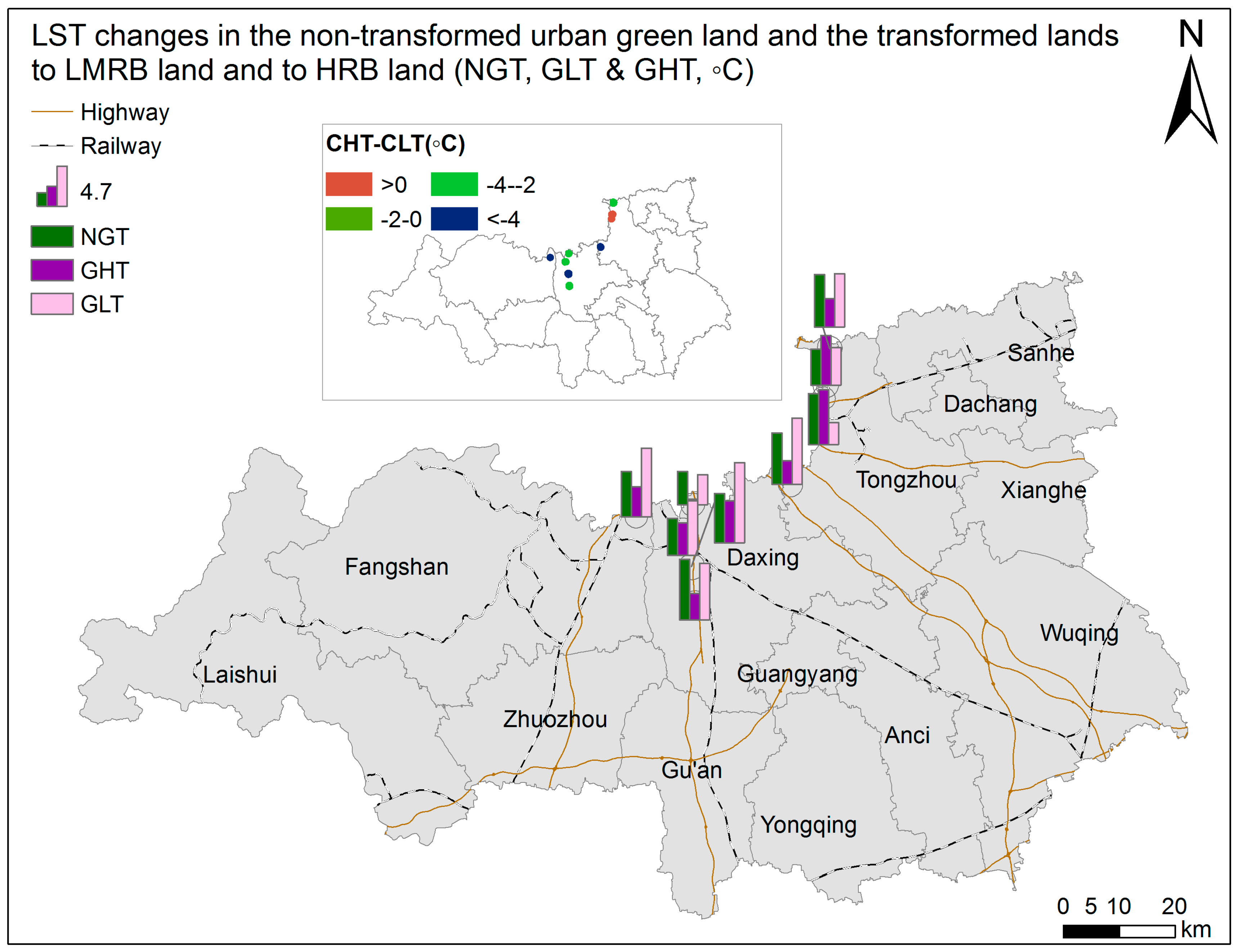
For the urban green land, the expected LST increase in the urban green land was on average 5.78 °C, which was raised by 0.012 °C and 0.003 °C due to the transformations to LMRB and HRB lands, respectively. At the local scale, the LST increases in the non-transformed urban green land and the transformation to HRB and to LMRB lands were all positive (

Table 5. Polygon-based LST comparisons between transformed land from urban green land to HRB land and urban green land to LMRB land among different buffer zones.

Average LST Changes (°C)	Among the Non-Transformed Urban Green Land and the Transformed Lands from Urban Green Land to HRB Land and Urban Green Land to LMRB Land
	300 (m)	500 (m)	700 (m)	1000 (m)	1500 (m)	2000 (m)	3000 (m)	5000 (m)
Sample number	2	2	2	3	7	9	12	17
Urban green land to HRB (GHT)	4.20	4.20	4.20	4.74	4.58	4.32	4.57	5.03
Urban green land to LMRB (GLT)	5.62	5.62	5.36	6.07	6.62	6.59	6.93	6.71
Non-transformed urban green land (NGT)	6.74	6.74	7.42	6.52	5.69	5.95	6.09	6.12
GHT − GLT (Number and percentage of samples where GHT − GLT < 0)	−1.42 (1, 50%)	−1.42 (1, 50%)	−1.16 (1, 50%)	−1.33 (2, 67%)	−2.04 (5, 71%)	−2.26 (7, 78%)	−2.36 (10, 83%)	−1.69 (13, 76%)
GHT − NGT (Number and percentage of samples where GHT − NGT > 0)	−2.54 (0, 0%)	−2.54 (0, 0%)	−3.22 (0, 0%)	−1.79 (1, 33%)	−1.11 (3, 43%)	−1.62 (3, 33%)	−1.52 (3, 25%)	−1.10 (5, 29%)
GLT − NGT (Number and percentage of samples where GLT − NGT > 0)	−1.12 (1, 50%)	−1.12 (1, 50%)	−2.06 (0, 0%)	−0.46 (1, 33%)	0.93 (4, 57%)	0.64 (6, 67%)	0.84 (8, 67%)	0.59 (11, 65%)

, Figure 7). Furthermore, the increase in the transformation to HRB land was lower than those in the non-transformed urban green land and the transformation to LMRB land over all of the buffers. For most of transformation to LMRB land, the LST increase was higher than that of the non-transformed urban green land, ranging from 0.11 °C to 3.59 °C.

4. Discussion

Regional temperature change is closely related to conversions among land uses [16,46,47,48] due to their different thermal properties [49], and is also strongly influenced in this study by changes in building morphology [29,50], e.g., building height. In accordance with the previous studies [17,19,51,52], the built-up land expansion from vegetated land has increased the regional surface temperature (Figure 6 and Figure 7). From 2010 to 2015, the built-up land in the study area has increased by 13.4%, which came mainly from the surrounding cropland and urban green land. Compared with these vegetated areas, the built-up area has a lower surface adobe and higher surface thermal capacity [53], which induces the higher surface temperature during the daytime (Figure 8). In contrast to these previous studies, this study further found that the cooling effects resulting from the building height change in the built-up land (Table 3, Figure 3 and Figure 4) partly canceled the heating effects due to the built-up land expansion from vegetated lands. This cooling effect was probably due to three reasons. Firstly, in comparison with LMRB land, the HRB land has a much lower horizontal active surface because of the larger spacing between high-rise buildings (Figure 9a, b). According to the China’s residential building code, the sunshine hour for each residence should be higher than 1 h, which indicates that larger building spacing is required to guarantee enough sunshine in each high-rise residence. Furthermore, the high-rise buildings cast more shadows on their surroundings [28], inducing a lower LST compared with that of the LMRB areas (Figure 8). Thirdly, as building height increases, air ventilation is altered, and the created wind ventilation pathways reduce the surface temperature in the HRB land.

Vegetation also influences the thermal impacts of built-up land expansion [54,55]. In our study, although most of the transformation from LMRB to HRB land decreased the regional LST, for some transformed areas, the LST increase in the transformed land was much higher than those in the surrounding non-transformed LMRB land. For example, in Case #1 (Figure 9a), where the HRB land was transformed from LMRB land, the LST increased by 6.47 °C from 2010 to 2015, whereas the LST increase in its surrounding non-transformed LMRB land was much lower (4.74 °C). This mainly resulted from the limited and sparse vegetation in these HRB lands. From the Gaofen image, this region was identified as HRB land in 2015, whereas the greening in this region had not been developed by the investigation time (Figure 9a). As a result, most of the HRB land was covered by an impervious surface with higher LST. That the LST increase in the transformed land from cropland to HRB land was higher than that of the surrounding transformed land to LMRB land could also be explained by this reason (Figure 9b).

5. Conclusions

This study investigated the built-up land expansion in the transition zone between two megacities in China through high spatial resolution images from SPOT5 and Gaofen2. It further explored the thermal impacts of built-up land expansion—especially the effect of building height change—through LST from Landsat images.

From 2010 to 2015, the built-up land in the study area expanded by 87.25 km² and 13.21 km² in 2D and 3D, respectively, which induced an opposite thermal effect for the regional surface temperature. For the expansion in 2D, the expansions of built-up land from cropland and urban green land, in general, had heating effects for the regional surface temperature, where the effects from the transformation to LMRB land appeared to be stronger than that of the transformation to HRB land. However, for the expansion in 3D, cooling effects were found. The transformation from LMRB to HRB land decreased the surface temperature, leading to an average decrease of 0.043 °C for the whole LMRB land. At the local scale, however, the decrease was much larger, ranging from 0.24 °C to 4.99 °C (45% on average). In addition, the opposite thermal effects were complicated by vegetation in the built-up land. Although this study only assessed the thermal impacts during summer, it can also provide insights for urban design because of the maximum of SUHI generally occurring in this season. Our results indicated that building height should be considered in the urban design for mitigating the thermal impacts of urbanization. The challenge of how to find an optimal combination of buildings with different heights and vegetation in the built-up land will be conducted in our further work. Furthermore, this study also demonstrates that building height change should also be considered when considering the thermal impact of urban area expansion, due to its potential cooling effects.

References

- World of Change: Global Temperature: Feature Articles. Available online: http://earthobservatory.nasa.gov/Features/WorldOfChange/decadaltemp.php?src=eoa-features (accessed on 10 March 2017).
- Team, C.W.; Pachauri, R.K.; Reisinger, A. Climate Change 2007: Synthesis Report; Intergovernmental Panel on Climate Change (IPCC): Geneva, Switzerland, 2007; p. 104. [Google Scholar]
- Oleson, K.W.; Monaghan, A.; Wilhelmi, O.; Barlage, M.; Brunsell, N.; Feddema, J.; Hu, L.; Steinhoff, D.F. Interactions between urbanization, heat stress, and climate change. Clim. Chang. 2015, 129, 525–541. [Google Scholar] [CrossRef]
- Jacob, D.J.; Winner, D.A. Effect of climate change on air quality. Atmos. Environ. 2009, 43, 51–63. [Google Scholar] [CrossRef]
- Kalnay, E.; Cai, M. Impact of urbanization and land-use change on climate. Nature 2003, 423, 528–531. [Google Scholar] [CrossRef] [PubMed]
- Lin, S.; Feng, J.M.; Wang, J.; Hu, Y.H. Modeling the contribution of long-term urbanization to temperature increase in three extensive urban agglomerations in China. J. Geophys. Res. Atmos. 2016, 121, 1683–1697. [Google Scholar] [CrossRef]
- Zhou, L.M.; Dickinson, R.E.; Tian, Y.H.; Fang, J.Y.; Li, Q.X.; Kaufmann, R.K.; Tucker, C.J.; Myneni, R.B. Evidence for a significant urbanization effect on climate in China. Proc. Natl. Acad. Sci. USA 2004, 101, 9540–9544. [Google Scholar] [CrossRef] [PubMed]
- Seto, K.C.; Fragkias, M.; Guneralp, B.; Reilly, M.K. A meta-analysis of global urban land expansion. PLoS ONE 2011, 6, e23777. [Google Scholar] [CrossRef] [PubMed]
- Yang, X.Y.; Li, Y.G.; Luo, Z.W.; Chan, P.W. The urban cool island phenomenon in a high-rise high-density city and its mechanisms. Int. J. Climatol. 2017, 37, 890–904. [Google Scholar] [CrossRef]
- Smoliak, B.V.; Snyder, P.K.; Twine, T.E.; Mykleby, P.M.; Hertel, W.F. Dense network observations of the twin cities canopy-layer urban heat island. J. Appl. Meteorol. Clim. 2015, 54, 1899–1917. [Google Scholar] [CrossRef]
- Wang, K.C.; Jiang, S.J.; Wang, J.K.; Zhou, C.L.; Wang, X.Y.; Lee, X. Comparing the diurnal and seasonal variabilities of atmospheric and surface urban heat islands based on the Beijing urban meteorological network. J. Geophys. Res. Atmos. 2017, 122, 2131–2154. [Google Scholar] [CrossRef]
- Deng, C.B.; Wu, C.S. Examining the impacts of urban biophysical compositions on surface urban heat island: A spectral unmixing and thermal mixing approach. Remote Sens. Environ. 2013, 131, 262–274. [Google Scholar] [CrossRef]
- Weng, Q.H. Thermal infrared remote sensing for urban climate and environmental studies: Methods, applications, and trends. Isprs. J. Photogramm. 2009, 64, 335–344. [Google Scholar] [CrossRef]
- Nichol, J.E.; Fung, W.Y.; Lam, K.S.; Wong, M.S. Urban heat island diagnosis using aster satellite images and ‘in situ’ air temperature. Atmos. Res. 2009, 94, 276–284. [Google Scholar] [CrossRef]
- Sun, Y.J.; Wang, J.F.; Zhang, R.H.; Gillies, R.R.; Xue, Y.; Bo, Y.C. Air temperature retrieval from remote sensing data based on thermodynamics. Theor. Appl. Climatol. 2005, 80, 37–48. [Google Scholar] [CrossRef]
- Chen, X.L.; Zhao, H.M.; Li, P.X.; Yin, Z.Y. Remote sensing image-based analysis of the relationship between urban heat island and land use/cover changes. Remote Sens. Environ. 2006, 104, 133–146. [Google Scholar] [CrossRef]
- Qiao, Z.; Tian, G.J.; Xiao, L. Diurnal and seasonal impacts of urbanization on the urban thermal environment: A case study of Beijing using modis data. Isprs. J. Photogramm. 2013, 85, 93–101. [Google Scholar] [CrossRef]
- Xu, H.Q.; Ding, F.; Wen, X.L. Urban expansion and heat island dynamics in the Quanzhou region, China. IEEE J. Stars 2009, 2, 74–79. [Google Scholar] [CrossRef]
- Zhao, M.Y.; Cai, H.Y.; Qiao, Z.; Xu, X.L. Influence of urban expansion on the urban heat island effect in Shanghai. Int. J. Geogr. Inf. Sci. 2016, 30, 2421–2441. [Google Scholar] [CrossRef]
- Zhou, D.C.; Zhao, S.Q.; Zhang, L.X.; Sun, G.; Liu, Y.Q. The footprint of urban heat island effect in China. Sci. Rep. 2015, 5. [Google Scholar] [CrossRef] [PubMed]
- Arnfield, A.J. Two decades of urban climate research: A review of turbulence, exchanges of energy and water, and the urban heat island. Int. J. Climatol. 2003, 23, 1–26. [Google Scholar] [CrossRef]
- Rizwan, A.M.; Dennis, Y.C.L.; Liu, C.H. A review on the generation, determination and mitigation of urban heat island. J. Environ. Sci. 2008, 20, 120–128. [Google Scholar] [CrossRef]
- Feizizadeh, B.; Blaschke, T. Examining urban heat island relations to land use and air pollution: Multiple endmember spectral mixture analysis for thermal remote sensing. IEEE J. Stars 2013, 6, 1749–1756. [Google Scholar] [CrossRef]
- Li, J.J.; Wang, X.R.; Wang, X.J.; Ma, W.C.; Zhang, H. Remote sensing evaluation of urban heat island and its spatial pattern of the shanghai metropolitan area, China. Ecol. Complex. 2009, 6, 413–420. [Google Scholar] [CrossRef]
- Zhou, B.; Rybski, D.; Kropp, J.P. The role of city size and urban form in the surface urban heat island. Sci. Rep. 2017, 7. [Google Scholar] [CrossRef] [PubMed]
- Buyantuyev, A.; Wu, J.G. Urban heat islands and landscape heterogeneity: Linking spatiotemporal variations in surface temperatures to land-cover and socioeconomic patterns. Landsc. Ecol. 2010, 25, 17–33. [Google Scholar] [CrossRef]
- Li, X.M.; Zhou, Y.Y.; Asrar, G.R.; Imhoff, M.; Li, X.C. The surface urban heat island response to urban expansion: A panel analysis for the conterminous United States. Sci. Total Environ. 2017, 605, 426–435. [Google Scholar] [CrossRef] [PubMed]
- Lindberg, F.; Grimmond, C.S.B. The influence of vegetation and building morphology on shadow patterns and mean radiant temperatures in urban areas: Model development and evaluation. Theor. Appl. Climatol. 2011, 105, 311–323. [Google Scholar] [CrossRef]
- Lindberg, F.; Grimmond, C.S.B. Nature of vegetation and building morphology characteristics across a city: Influence on shadow patterns and mean radiant temperatures in London. Urban Ecosyst. 2011, 14, 617–634. [Google Scholar] [CrossRef]
- Radhi, H.; Fikry, F.; Sharples, S. Impacts of urbanisation on the thermal behaviour of new built up environments: A scoping study of the urban heat island in Bahrain. Landsc. Urban Plan. 2013, 113, 47–61. [Google Scholar] [CrossRef]
- Wong, N.H.; Jusuf, S.K.; Syafii, N.I.; Chen, Y.X.; Hajadi, N.; Sathyanarayanan, H.; Manickavasagam, Y.V. Evaluation of the impact of the surrounding urban morphology on building energy consumption. Sol. Energy 2011, 85, 57–71. [Google Scholar] [CrossRef]
- Emmanuel, R.; Johansson, E. Influence of urban morphology and sea breeze on hot humid microclimate: The case of Colombo, Sri Lanka. Clim. Res. 2006, 30, 189–200. [Google Scholar] [CrossRef]
- Giridharan, R.; Ganesan, S.; Lau, S.S.Y. Daytime urban heat island effect in high-rise and high-density residential developments in Hong Kong. Energy Build. 2004, 36, 525–534. [Google Scholar] [CrossRef]
- Feng, Z.M.; Yang, L.; Yang, Y.Z.; You, Z. The process of population agglomeration/ shrinking and changes in spatial pattern in the Beijing-Tianjin-Hebei metropolitan region. J. Geo-Inf. Sci. 2013, 15, 11–18. [Google Scholar] [CrossRef]
- Chang, N.B.; Han, M.; Yao, W.; Chen, L.C.; Xu, S.G. Change detection of land use and land cover in an urban region with SPOT-5 images and partial lanczos extreme learning machine. J. Appl. Remote Sens. 2010, 4, 043551. [Google Scholar]
- Pongracz, R.; Bartholy, J.; Dezso, Z. Remotely sensed thermal information applied to urban climate analysis. Adv. Space Res. 2006, 37, 2191–2196. [Google Scholar] [CrossRef]
- Liu, J.Y.; Kuang, W.H.; Zhang, Z.X.; Xu, X.L.; Qin, Y.W.; Ning, J.; Zhou, W.C.; Zhang, S.W.; Li, R.D.; Yan, C.Z.; et al. Spatiotemporal characteristics, patterns, and causes of land-use changes in China since the late 1980s. J. Geogr. Sci. 2014, 24, 195–210. [Google Scholar] [CrossRef]
- Liu, J.Y.; Liu, M.L.; Tian, H.Q.; Zhuang, D.F.; Zhang, Z.X.; Zhang, W.; Tang, X.M.; Deng, X.Z. Spatial and temporal patterns of China’s cropland during 1990–2000: An analysis based on Landsat TM data. Remote Sens. Environ. 2005, 98, 442–456. [Google Scholar] [CrossRef]
- Liu, J.Y.; Zhang, Z.X.; Xu, X.L.; Kuang, W.H.; Zhou, W.C.; Zhang, S.W.; Li, R.D.; Yan, C.Z.; Yu, D.S.; Wu, S.X.; et al. Spatial patterns and driving forces of land use change in China during the early 21st century. J. Geogr. Sci 2010, 20, 483–494. [Google Scholar] [CrossRef]
- Liasis, G.; Stavrou, S. Satellite images analysis for shadow detection and building height estimation. ISPRS J. Photogramm. 2016, 119, 437–450. [Google Scholar] [CrossRef]
- Cheng, F.; Thiel, K.H. Delimiting the building heights in a city from the shadow in a panchromatic SPOT-image.1. Test of 42 buildings. Int. J. Remote Sens. 1995, 16, 409–415. [Google Scholar] [CrossRef]
- Shettigara, V.K.; Sumerling, G.M. Height determination of extended objects using shadows in SPOT images. Photogramm. Eng. Remote Sens. 1998, 64, 35–44. [Google Scholar]
- Weng, Q.H.; Lu, D.S.; Schubring, J. Estimation of land surface temperature-vegetation abundance relationship for urban heat island studies. Remote Sens. Environ. 2004, 89, 467–483. [Google Scholar] [CrossRef]
- Sobrino, J.A.; Jimenez-Munoz, J.C.; Paolini, L. Land surface temperature retrieval from Landsat TM 5. Remote Sens. Environ. 2004, 90, 434–440. [Google Scholar] [CrossRef]
- Ding, F.; Xu, H.Q. Comparison of three algorithms for retriveving land surface temperature from Landsat TM thermal infrared band. J. Fujian Norm. Univ. (Nat. Sci. Ed.) 2008, 24, 91–96. [Google Scholar]
- Hale, R.C.; Gallo, K.P.; Owen, T.W.; Loveland, T.R. Land use/land cover change effects on temperature trends at U.S. Climate normals stations. Geophys. Res. Lett. 2006, 33. [Google Scholar] [CrossRef]
- Jones, P.D.; Groisman, P.Y.; Coughlan, M.; Plummer, N.; Wang, W.C.; Karl, T.R. Assessment of urbanization effects in time-series of surface air-temperature over land. Nature 1990, 347, 169–172. [Google Scholar] [CrossRef]
- Jones, P.D.; Lister, D.H.; Li, Q. Urbanization effects in large-scale temperature records, with an emphasis on China. J. Geophys. Res. Atmos. 2008, 113. [Google Scholar] [CrossRef]
- Kuang, W.H.; Dou, Y.Y.; Zhang, C.; Chi, W.F.; Liu, A.L.; Liu, Y.; Zhang, R.H.; Liu, J.Y. Quantifying the heat flux regulation of metropolitan land use/land cover components by coupling remote sensing modeling with in situ measurement. J. Geophys. Res. Atmos. 2015, 120, 113–130. [Google Scholar] [CrossRef]
- Li, J.X.; Song, C.H.; Cao, L.; Zhu, F.G.; Meng, X.L.; Wu, J.G. Impacts of landscape structure on surface urban heat islands: A case study of Shanghai, China. Remote Sens. Environ. 2011, 115, 3249–3263. [Google Scholar] [CrossRef]
- Ren, G.Y.; Zhou, Y.Q.; Chu, Z.Y.; Zhou, J.X.; Zhang, A.Y.; Guo, J.; Liu, X.F. Urbanization effects on observed surface air temperature trends in north China. J. Clim. 2008, 21, 1333–1348. [Google Scholar] [CrossRef]
- Weng, Q. A remote sensing-gis evaluation of urban expansion and its impact on surface temperature in the Zhujiang delta, China. Int. J. Remote Sens. 2001, 22, 1999–2014. [Google Scholar]
- Zhang, Y.S.; Balzter, H.; Wu, X.C. Spatial-temporal patterns of urban anthropogenic heat discharge in Fuzhou, China, observed from sensible heat flux using Landsat TM/ETM plus data. Int. J. Remote Sens. 2013, 34, 1459–1477. [Google Scholar] [CrossRef]
- Weng, Q.H.; Lu, D.S. A sub-pixel analysis of urbanization effect on land surface temperature and its interplay with impervious surface and vegetation coverage in Indianapolis, United States. Int. J. Appl. Earth Obs. 2008, 10, 68–83. [Google Scholar] [CrossRef]
- Weng, Q.H.; Rajasekar, U.; Hu, X.F. Modeling urban heat islands and their relationship with impervious surface and vegetation abundance by using ASTER images. IEEE Trans. Geosci. Remote Sens. 2011, 49, 4080–4089. [Google Scholar] [CrossRef]
Figure 1.
(a) SPOT5 and Gaofen2 image tiles used in this study; (b) land use distribution in the study area for the year 2015. LMRB: low- and moderate-rise building; HRB: high-rise building.
Figure 2.
The built-up land expansion from 2010 to 2015.
Figure 3.
The area percentages among different Tni level changes in the non-transformed LMRB land, the study area, and the transformed land from LMRB to HRB.
Figure 4.
LST changes in the transformed land, from LMRB to HRB (LHT) and non-transformed LMRB land (NLT), among different samples at a 2 km buffer zone.
Figure 5.
The area percentages among different Tni level changes in the transformed lands from cropland to LMRB land, from cropland to HRB land, from urban green land to LMRB land, from urban green land to HRB land, non-transformed cropland and non-transformed urban green land.
Figure 6.
LST changes in the non-transformed cropland (NCT) and the transformed land from cropland to LMRB (CLT) land, and from cropland to HRB land (CHT), among different samples at a 2 km buffer zone.
Figure 7.
LST changes in the non-transformed urban green land (NGT) and the transformed land from urban green land to LMRB land (GLT), and from urban green land to HRB land (GHT), among different samples at a 2 km buffer zone.
Figure 8.
Mean LSTs among different land use types.
Figure 9.
Comparisons (a): between LST changes in the non-transformed LMRB land (NLT) and the transformed land from LMRB to HRB (LHT), also Case #1 in Figure 4; and (b): between LST changes in the transformed lands from cropland to LMRB (CLT) and from cropland to HRB (CHT), also Case #2 in Figure 6.