Low-Carbon Planning and Design in B&R Logistics Service: A Case Study of an E-Commerce Big Data Platform in China

Abstract

The concept of sustainable development requires us to explore a completeness model of low carbon transport and service in the light of the advancement of changes in world cooperation policy. Various kinds of carbon constraints not only limit emissions of contaminants from E-commerce Enterprise of different countries, but they also ensure the market activity around the Belt and Road, so as to avoid the implementation reducing the company’s profits significantly. This paper discusses of the strictest periodic low-carbon constraints_(PLC) and the expansion of the mainstream with three relatively weak attributes—cumulative_(CLC), full cycle_(FCLC), and volatility_(VLC)—taking into account the offline delivery of lead time and the online relationship between supply and demand on the platform. We have established four decision models with different carbon confinement intensities and inferred the impact of more detailed carbon constraints on E-commerce delivery strategies. The appropriate operational decisions, under a wide spectrum of carbon constraints, help e-companies develop scientific delivery plans, and provide some inspiration for the promotion of low carbon economy system construction and environmental significance.

1. Introduction

The “Belt and Road” initiative (“B&R”) provides new opportunities for achieving the goals of the United Nations sustainable development and offers a new paradigm for global win-win cooperation. According to the IPCC2014 report, global greenhouse gas emissions have risen to unprecedented levels [1]. This raises the point: in order to effectively reduce carbon dioxide emissions and achieve sustainable development of the population, environment and resources, the United Nations has developed a set of mechanisms such as carbon credits, carbon offset, carbon tax and so on. At the Copenhagen Conference in 2009, the Chinese government put forward the goal compared to 2005: a 40% reduction in carbon dioxide emissions per unit by 2020. Subsequently, the “low carbon” penetrates into all aspects of China’s economic and social development, and inevitably integrates into China’s “B&R” policy [2]. On the basis of the relationship between e-commerce and the real economy, the strategic area decision-makers create “government leading, social participation, and market allocation” along the way. Using a the cross-border e-commerce platform, specialized cloud logistics system, Internet finance, and other components of the new e-commerce model, the effect in both the short and long term has been demonstrated [3]. In the short-term, this new model will be helpful to adequately reflect the economic characteristics of the strategic area, cultivate new consumption growth points, and increase employment channels and social welfare; in the long-term, it will be beneficial to reducing the business costs of narrowing the regional gap in the backward areas and integrate consumer demand in time to improve product competitiveness.

After a five-year investigation and demonstration, the United Nations Intergovernmental Panel on Climate Change (IPCC), issued a fifth assessment report, which argues that human activity has been a central factor in global warming throughout the twentieth century. In 2015, most parts of the world were hit by extreme weather, on account of global warming [4]. According to the “China Climate Bulletin 2015” from the China Meteorological Administration in January 2016, it was said that 2015 saw the highest annual average temperature of the years of recorded modern weather data. The continued rise in global temperatures has triggered sea-level rise, glacier melting, and extreme weather, which has had a serious impact on the Earth’s ecosystem and human life. The El Niño phenomenon has intensified due to the greenhouse effect, and the possibility of frequent occurrences are growing with the cycle showing a shortening trend. The reduction in greenhouse gas emissions and easing of the greenhouse effect are imminent [5,6].

As the new century has arrived, despite more frequent global financial crisis, the rationalization of the economic structure has become prominently visible, and the global economy has grown [7]. Economic development has contributed to the increase in consumer spending, and the globalization of the economy has increased the global circulation of commodities. However, the production, transportation, storage, and consumption of goods also have a serious impact on the environment. The “low-carbon economy” of low-energy and sustainable green ideas has become the focus of scholars and the general public in the context of the persistence of global warming. Sustainable development has raised higher demands and challenges. The “Stern report” shows that a global annual investment of 1% of GDP used to deal with such problems can avoid the future annual 5–20% GDP losses and, thus, calls for a global transition to a low carbon economy [8]. Relevant governments, organizations, businesses and institutions also claim to be reducing their own carbon emissions. The China National Development and Reform Commission made it clear that China will invest thirty million dollars to resist carbon emissions by 2020 [9]. At the same time, the Chinese government promulgated relevant carbon emission policies and financial subsidies and other measures to promote China’s sustainable development of the basic national policy to be implemented smoothly because of their responsibility and obligations. Energy-saving emission reduction is bound to the future development of the trend. As the vanguard of emission reductions, the European Union has been acting for many years, and policies have been introduced to promote carbon reduction, such as carbon taxes, carbon trading, and carbon total control [10]. With the effect of a growing greenhouse effect, higher requirements for the carbon emission reduction have been put forward.

As an extremely important part of supply chain activities, the carbon emissions involved in the delivery of goods are no less than the production of goods, and may even occupy a larger proportion. Delivery issues related to carbon emissions mainly come from transportation, for example shipping, railways, trucks, and other modes of transport [11]. The global supply chain increases the mileage of material delivery, resulting in a very high level of carbon emissions. The efficiency of delivery will not only affect the overall profitability and development of the supply chain, and determine the economic activity of the supply chain, but also play a decisive role in the overall carbon supply to the supply chain [12]. In order to reduce the supply chain of carbon emissions, the material delivery process of carbon emissions has attracted the attention of experts and the public. In recent years, the research on the emission reduction in the process of logistics has been increasing year by year. How to control carbon emissions has created widespread concern and become an important issue in both industrial and academic fields. As long as there are delivery activities, there will be transport and carbon emissions, which have been of concern. The problem of carbon emissions in the study of the logistics process has become regular and systematic, but there is a lack of innovation in the research paradigm [13]. Research on the mathematical model, such as distribution methods, delivery strategies, and other carbon considerations that take into account other factors have long been on the agenda. For example, the JD.com global online shopping site launched their “global sales” business, then released their online site in English and Russian on 11 June 2015. As one of the largest self-owned business enterprises, JD’s internationalization seems a bit late; after all, Alibaba [14] had set up a quick sell platform, and established the layout of exports of cross-border electricity businesses as early as 2010. Comprehensive transportation is a crucial and final touch between consumers and e-retailers, and a widely used phrase in electronic commerce links between online retailers and consumers in the process of logistics distribution.

The main contents of this paper include the following aspects:

(i)

Section 2 reviews the research literature on the supply chain model under the carbon constraint, including the research on the transportation and the retailer’s delivery, and the Bender’s decomposition method used in this paper to solve the mathematical model.

(ii)

The model construction of the retailer delivery strategy under the periodic carbon constraints is considered in Section 3. As the basic model of this paper, the periodic low-carbon constraints model (PLC) imposes a carbon emission constraint on the planning of each decision cycle because it is not a complicated design for the research approach to build and calculate a model.

(iii)

A study on the delivery strategy model of e-commerce retailers considering the relationship between early stage and supply and demand with three kinds of expansion carbon constraints. The low-carbon delivery strategy under the periodic local carbon policy restriction is a decision model with the highest intensity constraints from the point of view of the mathematical dynamic planning. In Section 4, the constraint intensity gradually relaxed, the paper obtains properties under different carbon constraint considering the lead time and delivery strategy model of supply and demand.

(iv)

Taking the JD.com global online shopping site as an example, the calculation experiment and simulation are carried out, and the feasibility and validity of the analytical method are illustrated by an example analysis, and some conclusions and relevant enlightenment are obtained according to the experimental results in the Section 5.

(v)

The conclusion and future prospects are shown in Section 6. This section summarizes the main research work and the conclusions of this paper, and points out the main contribution and the research work that needs to be carried out further.

2. Literature Review

2.1. Supply Chain Model with Carbon Emissions

According to the Coase theory [15], the goal of carbon emission management is not only to eliminate greenhouse gas emissions, but also to ensure the level of greenhouse gas emissions in a reasonable range. From the perspective of academic research, the current distributions of carbon emissions are free and public auction and sale [16]. Burtraw et al. [17] systematically delineated the allocation of carbon emissions rights in regional power companies (Regional Greenhouse Gas Initiative, RGGI), which are involved in regional greenhouse gas emission reduction. Sterner et al. [18] construed the effect of adjusting the initial share of carbon emission rights on firms and analyzed the effects of different allocation schemes on the incentive mechanism for emission reductions using a simple multi-period model. Carbon trading quota allocation, trading mechanism and punitive carbon tax mechanism are difficult points to implement in the future [19].

The carbon trading market is a generic term for greenhouse gas emissions trading and various financial activities and transactions related to such activities [20]. According to the current low carbon problem study, the major trading products on the world carbon market are shown in

Table 1. Transactions of global carbon market.

The Type of Carbon Trading	Items	Shortened Form	The Connotation of Trading Products
Mandatory emission reduction transaction	Quota transaction [19,22]	CERs [21,23]	Certified emission reduction
		EUAs [24,25,26,27]	European Union emission quota
		AAUs [28]	Assigned amount units
	Program trading	ERUs [29]	Emission reduction units
		RMUs	Carbon sink mitigation units
Voluntary emission reduction transaction	Quota transaction [20]	CFI	Carbon financial instrument
	Odd-lot trading	Carbon Offsets	Carbon offsets
	Program trading [30]	VERs [31,32,33,34,35]	Voluntary emission reduction
		VCS [36,37,38]	Voluntary carbon standard

. The international community has formed a mandatory trading system represented by the European Union and a voluntary trading system represented by the Chicago climate exchange. Dales [21] proved the idea of emission trading on the basis of the Coase theorem and externality theory of environmental pollution, and then defined the boundary of emission rights. Bernard [22] illustrated a strategy game between Russia and competitive developing countries on the basis of an international emission permit market in the Kyoto Protocol. Weikard et al. [23] assessed a framework for carbon emission reduction negotiations based on carbon trading, guaranteeing the stability and feasibility of the international carbon emission reduction agreement. According to Egenhofer [24], the European Union’s carbon emissions trading scheme and assessment confirmed that the mechanism was an effective economic tool. Perdan et al. [25] conducted a comprehensive overview of a global carbon trading plan by that time. Daskalakis et al. [26] found that the actual trading volume and trading situation of the European Union’s carbon trading market was not ideal. Chaabane et al. [27] formulated the design of supply chain networks under the emission trading mechanism. Paltsev et al. [28] evaluated the US greenhouse gas quota and trading plan and analyzed the Emissions Forecasting and Policy Analysis (EPPA) model.

In supply chain management, the research of the e-commerce delivery model overlaps with many research directions. From an economic point of view, the transport path problem includes problems, such as vehicle routing problems, scheduling path problems, and integrated logistics system path problems. Ulku et al. [29] believed that the combined truck transport model could effectively reduce the transportation cost and CO₂ emission. Liao et al. [31] pointed out that replacing combined transport with long-distance truck transport can significantly reduce carbon emissions. In the traditional delivery strategy model, the research on carbon emissions is often overlooked, and cost profit model are generally valued. In recent years, some researchers have made contributions to this, Choi [30] obtained the selection of supply chain under carbon caps, and explored the different forms of carbon tax effect on the overall design of the supply chain. Jin [32] investigated logistics transportation mode selection of the Wal-Mart supply chain, a large American supplier, under all types of carbon policies. Tsai et al. [33] made a sensitivity analysis of the carbon footprint of each node in the supply chain, thus optimizing the transportation path, achieving the goal of reducing emission and costs. Kim [34] compared to CO₂ emissions of a combined transport and the road transportation system. Demir et al. [35] reviewed the recent studies about green road transport of goods.

In addition, according to the characteristics of the required delivery of the product, researchers have conducted in-depth analyses of the different products for the time dependence, such as perishables, industrial reagents, and so on. Soysal et al. [36] addressed the problem of modeling food logistics networks under carbon constraints, considering an international beef logistics supply chain network. Chen et al. [37] analyzed the food delivery at a variety of temperatures with time requirements. Mehmet et al. [38] stated the problem of inventory path considerations for perishable products. The study of product characteristics is also very worthy of in-depth study so as to improve transport efficiency, and it is necessary for reducing inventory costs.

2.2. Bender’s Decomposition

In view of the deepening research on carbon emissions, the models are becoming more and more complicated, as they are NP-hard models after being integrated into carbon emissions, with considerable difficulty in finding solutions. Some researchers have focused their attention on solving algorithms of these problems (Demir et al., 2014 [39]; Konur 2014 [40]; Tiwari et al., 2015 [41]; Brandenburg 2015 [42]; Jabir et al., 2015 [43]).

After Bender proposed the decomposition algorithm in 1962, the method was often used in the mixed integer programming algorithm [44]. The idea of the algorithm is to decompose the problem into two parts containing the main problem (MP) and the sub-problem (SP) so as to obtain an iterative solution. The MP is used to obtain the integer feasible solution and input the result into the SP. Linear problems with only real variables can be obtained through this process. The dual model of the sub-problem can deduce the linear optimal solution, and add the corresponding constraint to the main problem, and then obtain the integer feasible solution iterations when the upper and lower bounds in the algorithm are the same or certain optimization accuracy to terminate the algorithm can be satisfied.

However, the Bender’s decomposition algorithm has shortcomings, like the general iterative algorithm; for example, the calculation is slow, and it is easy to fall into the local optimal solution. A large number of scholars have analyzed the structure of the Bender’s decomposition algorithm, and put forward a series of improvements, which are divided into three types:

Type I

The main problem constraint model is intensified. From the solution of the decomposition algorithm, we can see that the purpose of the iterative process is to obtain more main problem constraints. If the results of each iteration can generate more compact and effective cutting plane, the efficiency of the algorithm is naturally improved (Fortz et al., 2009 [45]; Bektaş 2012 [46]; Saharidis et al., 2010 [47]; Wu et al., 2003 [48]).

Type II

A more feasible integer variable cutting plane. Some scholars put forward the idea of combining intelligent algorithms, which means that the more feasible solutions that exist, the more tangent planes. Naturally, the generation of a large number of cutting planes can greatly reduce the solution of the main problem (Rei et al., 2009 [49]; Poojari et al., 2009 [50]).

Type III

Effective cutting plane selection. Different from the previous two types, the method selects the tangent planes to obtain a more effective cutting plane. However, the method requires a significant amount of time to determine the effectiveness of the cutting plane (Yang et al., 2012 [51]).

Bender’s decomposition can only solve mixed integer linear programming, and it is powerless for mixed integer nonlinear programming. To address this situation, Prof. Geoffrion [52] of the University of California, extended it to the field of non-linear programming, which is generally referred to as Generalized Bender’s Decomposition (GBD), and the details are also available for reference (Lasdon 1970 [53]; Floudas 1995 [54]).

3. Periodic Low-Carbon Constraints Model (PLC)

Divide the cycle of T into consecutive service sub-cycles denoted by i. The whole online supply chain problem can be divided into two parts: the first part shows that the consumers select the goods through an electric business platform according to their own needs; the other part conveys that e-commerce retailers take online orders from customers and handle the process of delivery. Consumers select products according to their preferences and send orders through e-commerce platforms, which are mapped to the supply chain on behalf of realizing the choice of e-commerce retailers. By considering the time sensitivity of the virtual supply and demand relationship between e-commerce retailers and consumers, we can find the total cost $C_t^p$, then choose the total cost $C_t^p$ of different goods according to the consumers in the market, and solve the probability ${\gamma }_t^p$ that the retailer will be selected by the probability $\phi \left(h\right)$ of a consumer’s time value function. The retailer’s demand $Q_i^p$ for product $p$ can be solved by ${\gamma }_t^p$. Consumer’s orders, as the input of the e-retailer service system, will be paid the minimum costs $C_t^p$ within demand time windows, combining ${\gamma }_t^p$. After receiving the order demand $Q_i^p$, the retailer needs to deliver it to the consumer according to his own lead time ∂. Since the delivery of a retailer requires a certain lead time $\partial$, orders within the period $\left(t_i^0,\left(t_i^m-\partial \right)\right)$ of service cycle $i$ are delivered at the end of the service week, and the order in the time period $\left(\left(t_i^m-\partial \right),t_i^m\right)$ will be delivered at the end of the next cycle, together with the order of the forward stage of the next cycle, in which delayed payments will have a certain impact on e-commerce retailers, which we use the price discount α to represent. The amount of orders that need to be delivered during the service cycle $i$ is $\left(Q_{i-1}^{p2}+Q_i^{p1}\right)$. We can obtain the total delivery cost $Z_i^k$ of the retailer, which is composed of transportation cost $C_i^k$ and loss cost $L_i$. Then, we can obtain the total profit function B, and then the goal of the model is to maximize B. The constraints of the model restrict the delivery of carbon emissions during transport, in addition to the time constraints and supply and demand.

As Figure 1 shows, consumers choose the appropriate e-commerce retailers to meet their needs, potentially implied by the supply and demand relationship between e-commerce retailers and consumers. At the same time, the retailer’s lead time can also affect the supply and demand; however, these are virtual for consumers who shop through the e-platform. We have come to the consumer’s choice of e-commerce retailers, considering the time value of the consumers for the product, the order delay, and so on, through the analysis. According to market conditions, consumers choose the product and select the retailer to supply indirectly and, potentially, while the occurrence of this event contains a probability. The lead time period and relationship between supply and demand not only affect the consumer’s time perception and the efficiency of receiving products, but also impact the order quantity, delivery cost, and ultimate profit of the retailer.

In this study we use the following symbols:

• $C_t^p$: The average total value of ordering the product $p$ for the consumer;
• ${\overline{c}}_p$: The average price of the commodity $p$ on the e-commerce platform;
• $c_p$: The average cost of the retailer’s product $p$;
• ${\delta }_n$: The average time value of the consumer n;
• ${\mu }_p$: The weighting index of the consumer’s time value for product p;
• $T_t^p$: The average delay time of the product for consumers;
• $q_t^p$: The average amount of orders placed by the consumer on the product $p$ during the period t;
• $i$: Service cycle number;
• $T$: Planning cycle;
• $T_i$: The time window of the service cycle $i$, $\left(t_i^0,t_i^m\right), i=1,2,\dots ,T$;
• $T_i^R$: The average transit time for the retailer to deliver to the consumer, in the service cycle i;
• $u$: The time of discharging for the goods after arrival at the consumer;
• $\partial$: The lead time of the retailer delivery;
• $n_i$: The average number of times a consumer receives a product within service period i;
• $f_k$: The fixed cost of transportation mode k;
• $v_k$: The variable cost of bulk product for transportation mode k;
• $D_n$: The distance that the retailer needs to transport to the consumer n;
• ${\overline{\rho }}_p$: The minimum density of goods transported by mode $k$ can provide;
• $e_k$: The carbon emission of transport mode $k$ delivers per kilometer of bulk products;
• $Q_{ik}^{np}$: The average number of products $p$ delivered for the consumer n for mode $k$ within cycle $i$;
• $E_i^{max}$: The largest unit of the carbon emission of product allowed by service cycle $i$.

3.1. Descriptive Process Model: Consumers Choose E-Commerce Retailers

The cost to the consumer is associated with the time-dependent variable, in addition to the quantity and the unit price of the ordered product. The delivery time is different for the consumer’s time-sensitive perception. The faster the order is received, the more satisfied the consumer will feel. A longer delay in delivery for consumers may reduce the potential psychological needs. The difference of online and offline purchase is essential: offline orders immediately meet the needs, but online orders are almost impossible to deliver instant gratification; thus, a weighting factor ${\delta }_n$ is given greater than 1 to represent the consumer’s timeliness value. ${\mu }_t^p$ represents the weighted coefficient of product $p$ for consumer time value and ${\mu }_t^p\ge 1$, so the time value of product $p$ is $\left({\mu }_t^p·{\delta }_n\right)$ for the consumer. The total value of ordering the product $p$ for the consumer is $C_t^p$, then:

$$C_t^p=\left({\overline{c}}_p+T_t^p·{\mu }_t^p·{\delta }_n\right)q_t^p$$

(1)

Let $T_i$ denote the time window of the service cycle $i$, $\left(t_i^0,t_i^m\right),i=1,2,\dots ,\mathrm{T}$, where $t_i^0$ and $t_i^m$, respectively, represent the start and end times of service cycle $i$; ∂ is the lead time of the retailer, and means that e-commerce retailers have the possibility of a shortage of supply and need to be restocked. $n_i$ calculates the number of times a consumer receives a product within service period $i$ and $u$ measures the time of discharging for the goods after arrival at the consumer. In this process, we ignore the details of the transport path factors during the delivery process, and the delivery time is represented by means of the total transportation time and unloading time. Due to the need for the last mile of delivery service, except for long-distance transport, if the order is presented within $\left(\left(t_i^m-\partial \right),t_i^m\right)$, the order will be delivered together with the order arriving at the next service cycle $\left(t_{i+1}^0,\left(t_{i+1}^m-\partial \right)\right)$. The consumer’s time from the beginning of submission of the order through the e-commerce platform to completion of the order can be expressed as:

$$T_t^D=\{\begin{array}{c}\left(t_i^m+\frac{1}{2}\left(T_i^R+n_i·u\right)\right)-t, t\in \left(t_i^0,\left(t_i^m-\partial \right)\right)\\ \left(t_{i+1}^m+\frac{1}{2}\left(T_{i+1}^R+n_{i+1}·u\right)\right)-t, t\in \left(\left(t_i^m-\partial \right),t_i^m\right)\end{array}$$

(2)

For e-commerce retailers, the time value of consumers is a random variable, because different consumers, even with the same perception, may have different reflections of time. Let $\mu$ denote the consumer’s time value and $f\left(\mu \right)$ denote the probability distribution function. For consumer n, the probability of its time value is $P\left\{\mu ={\mu }_n\right\}=\phi \left(n\right)$. In addition, we also need to assume that consumers can find the products in the market price and the methods of delivery are different for e-commerce retailers, with the purpose that consumers can find the right e-commerce retailers at any time according to their own needs. g and x, respectively, represent selected e-commerce retailers and other unselected e-commerce retailers, and it is easy to understand that g does not equal x. According to these parameters, we can obtain the probability of the consumer’s choice retailer g, and supply product p, within t:

$${\gamma }_t^p=P\left\{C_t^{p,g}\le C_t^{p,x},\forall x\ne g\right\}={\displaystyle \sum }_{n}P\left\{C_t^{p,g}\le \min C_t^{p,x}\right\}·\phi \left(n\right)$$

(3)

From the above formulas, it can be seen that consumer choice of e-commerce retailers is a time-dependent process. In addition, it is related to consumers’ needs and e-commerce retailers’ abilities. Consumer demand $q_t^p$ for product $p$ is exogenous within t, and related with time $t_i^0$ and $t_i^m$. The number of product $p$ that a retailer needs to deliver to the consumer can be expressed as $Q_t^p=q_t^p·{\gamma }_t^p$. Thus, consumer aggregate demand $Q_i^p$ for product $p$ in the service cycle can be expressed as the following formula:

$$Q_i^p={\displaystyle {\displaystyle \sum }_{t=t_i^0}^{t_i^m}}{Q}_t^p={\displaystyle {\displaystyle \sum }_{t=t_i^0}^{t_i^m}}{q}_t^p·{\gamma }_t^p$$

(4)

In a word, consumers will choose the best retailer to supply the goods according to their own needs, and this selection process is closely related to the time window. For this reason, the time value is a variable that must be considered.

3.2. The Sustainable Profit Function of the E-Retailer from the E-Commerce Platform

It is possible to ensure the amount of goods the retailer needs to distribute. Then, we can confirm the cost of the retailer’s delivery and the profits. The retailer begins to deliver orders submitted by consumers under service cycle i, and which orders belong to deferred delivery from the last cycle. The cost of delivery is mainly composed of the transportation process and the delay. Transport cost functions include fixed and variable transportation costs. The fixed transportation cost comes mainly from the labor cost and the depreciation expense of the transportation tool; variable transportation costs for early dispatch and transportation fuel derive from energy consumption, haul distance, means of transport, speed, and road conditions.

The number of consumer demand for product $p$ in service cycle $i$ is labeled as $Q_i^p$, and then we can set the order quantity $Q_i^{p1}$ in the period of $\left(t_i^0,\left(t_i^m-\partial \right)\right)$, and the order quantity $Q_i^{p2}$ in $\left(\left(t_i^m-\partial \right),t_i^m\right)$; then we obtain $Q_i^p=Q_i^{p1}+Q_i^{p2}$. According to our definition, e-commerce retailers need to give a certain price compensation for orders, denoted by $Q_i^{p2}$. Assuming that different orders have different discount rates, the discount rate is in a quantitative relationship with the order quantity, using α to represent the discount rate: $\alpha =f(Q_i^{p2})$. The transportation cost $C_i^k$ and the loss cost $L_i$ with the selection of transport mode $k$ at service cycle i, can be expressed as:

$$C_i^k=f_k+v_k·{\displaystyle {\displaystyle \sum }_{n=1}^N}{{\displaystyle \sum }}_{\forall p}{D}_n·(Q_{\left(i-1\right)k}^{np2}+Q_{ik}^{np1})$$

(5)

$$L_i=\alpha ·{\overline{c}}_p·Q_i^{p2}$$

(6)

$$Q_{ik}^{np}=Q_{\left(i-1\right)k}^{np2}+Q_{ik}^{np1}$$

(7)

where $f_k$ is the fixed cost of transportation mode k, $v_k$ marks the variable cost of the bulk product for transportation mode k, and $D_n$ represents the distance that the retailer needs to transport to consumer n.

According to the above description, it can be determined that the total delivery cost function $Z_i^k$ of the retailer in service cycle $i$ using transport tool $k$ can be expressed as follows:

$$Z_i^k=C_i^k+\alpha ·{\overline{c}}_p·Q_i^{p2}=f_k+v_k·{\displaystyle {\displaystyle \sum }_{n=1}^N}{{\displaystyle \sum }}_{\forall p}{D}_n·\left(Q_{\left(i-1\right)k}^{np2}+Q_{ik}^{np1}\right)+f\left(Q_i^{p2}\right)·{\overline{c}}_p·Q_i^{p2}$$

(8)

It can be seen from the formula that the delivery cost of the retailer in service cycle $i$ is directly related to the mode of transport, the transport mileage, the bulk density of the transport product, and the delivery window of the product. Then, the profit function of the retailer throughout the study period is B:

$$\mathrm{B}={\displaystyle {\displaystyle \sum }_{i=1}^T}({{\displaystyle \sum }}_{\forall p}\left({\overline{c}}_p-c_p\right)·Q_i^p)-{\displaystyle {\displaystyle \sum }_{i=1}^T}{\displaystyle {\displaystyle \sum }_{k=1}^K}{Z}_i^k$$

(9)

where $c_p$ is the retailer’s price per unit of product p.

The volume and density of the product are expressed by $v$(v $>0$) and $\rho \left(\rho >0\right),$ respectively. The charging standard for the transport mode is calculated based on the product’s bulk density [55]. The purpose is to limit the volume of the low density product. Bulk density $w_p$ can be defined by the following formula:

$$w_p=v\max \left\{\rho ,{\overline{\rho }}_p\right\}$$

(10)

where ${\overline{\rho }}_p\left({\overline{\rho }}_p\ge 0\right)$ indicates that the transport mode $k$ can provide the minimum density of the goods to be transported. If ${\overline{\rho }}_p=0$, then the actual weight of the product will be used to determine the transportation cost of transport mode k. In service cycle i, the bulk product of the total product that the retailer needs to deliver can be expressed by the following formula:

$$W_i={\displaystyle \sum }_{\forall p}{Q}_i^p·w_p={\displaystyle \sum }_{\forall p}{Q}_i^p·v\max \left\{\rho ,{\overline{\rho }}_p\right\}$$

(11)

In order to maintain the transport flexibility of the transport mode k, it is possible to provide transport services during the service cycle and must ensure that the bulk of the products to be transported does not exceed the maximum capacity of the transport mode. Let ${\theta }_i^k$ be a two-dimensional variable, in which ${\theta }_i^k=1$ when transport mode $k$ is selected in service cycle i, ${\theta }_i^k=0$, and vice versa. Then, the total capacity of the product to be delivered within service period $i$ can be expressed as:

$$w_{ik}={\displaystyle {\displaystyle \sum }_{n=1}^N}{{\displaystyle \sum }}_{\forall p}({\displaystyle {\displaystyle \sum }_{t=t_{i-1}^m-\partial }^{t_{i-1}^m}}{Q}_{i-1}^{p2}+{\displaystyle {\displaystyle \sum }_{t=t_i^0}^{t_i^m-\partial }}{Q}_i^{p1})·w_p$$

(12)

Let ${\overline{w}}_k$ be the maximum transport bulk of transport mode k. This constraint can be expressed as follows:

$$\left({\theta }_i^k·{\overline{w}}_k-w_{ik}\right)\ge 0$$

(13)

Then, regardless of the carbon constraint in the transport process at the time of delivery, the profit maximization planning model of the retailer throughout the planning period T can be described as follows:

$$\mathrm{Max}\mathrm{B}={\displaystyle {\displaystyle \sum }_{i=1}^T}\left({{\displaystyle \sum }}_{\forall p}\left({\overline{c}}_p-c_p\right)·Q_i^p\right)-{\displaystyle {\displaystyle \sum }_{i=1}^T}{\displaystyle {\displaystyle \sum }_{k=1}^K}{Z}_i^k$$

(14)

$$\mathrm{s}.\mathrm{t}.\{\begin{array}{c}\left({\theta }_i^k·{\overline{w}}_k-w_{ik}\right)\ge 0\\ t_{i+1}^0=t_i^m\\ {\displaystyle {\displaystyle \sum }_{i=1}^T}(t_i^m-t_i^0)=T\\ t_i^0,t_i^m>0 \forall i\end{array}$$

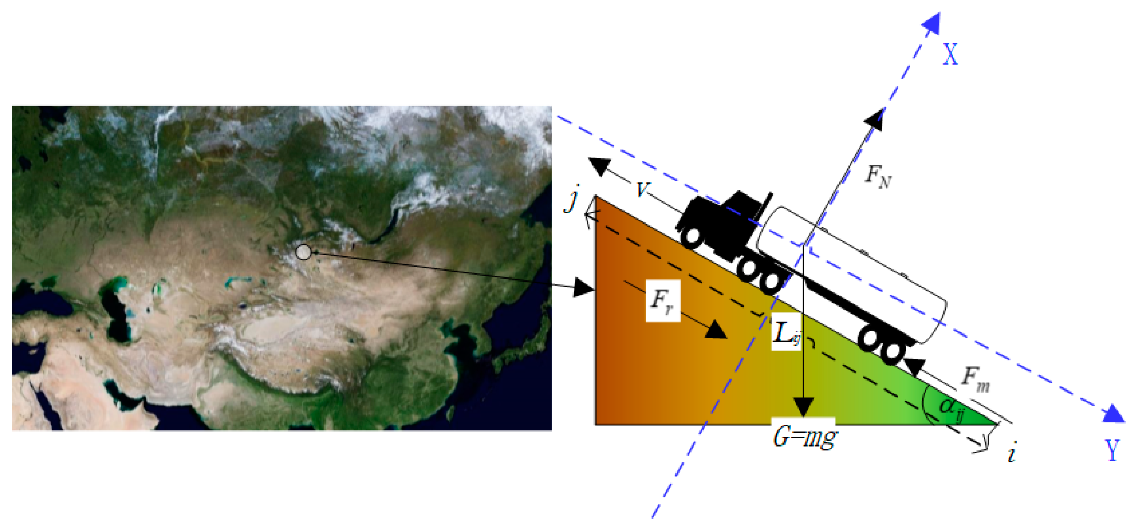
Flight conditions are relatively clear and simple, so air transport carbon emissions can be accurately estimated by fuel, time, and speed. In view of complex ground traffic, the landforms of various countries are diverse and uneven, so the carbon emissions statistics should take full account of the pavement characteristics [56]. As shown in Figure 2, we magnify the location along the B&R area, assuming that the slope of the road surface is ${\alpha }_{ij}$. Ground resistance is $F_r$. Locomotive power is expressed as $F_m$. $G=mg$ is the weight of the vehicle and cargo. $F_N$ represents the ground support force. The speed of the vehicle is marked as $v_{ij}$ and the driving distance is $L_{ij}$ from point $i$ to $j$. Based on the concepts of Newton’s laws, ${{\displaystyle \sum }}^{}{F}_x=m{a}_x\Rightarrow F_m-F_r-G·sin{\beta }_{ij}=0$ and ${{\displaystyle \sum }}^{}{F}_y=m{a}_y\Rightarrow N-G·cos{\beta }_{ij}=0$. The vehicle engine needs to do work $W_{ij}=F_m{L}_{ij}$. The total carbon emission is calculated as: $E_{ij}=e_1\times e_2\times {{\displaystyle \sum }}^{}{W}_{ij}$, in which the amount of fuel supporting ${{\displaystyle \sum }}^{}{W}_{ij}$ is deduced by $e_1$ (gallons/J). The amount of carbon emission per unit of power is given by $e_2$ (kg of ${\mathrm{CO}}_2$/gallon).

3.3. The Delivery Model for Periodic Low-Carbon Constraints

Periodic carbon constraints are defined as the amount of carbon quotas allocated by an enterprise, to the extent that carbon emissions in each sub-cycle cannot exceed the assigned amount. The amount of carbon emissions in each delivery cycle cannot exceed the amount of carbon allowed, and the remaining carbon limits for the previous cycle cannot be transferred to the next cycle. This is a very restrictive constraint. Let $E_i^{max}$ denote the carbon emissions of the maximum unit density product allowed by service cycle i. The $E_i^{max}$ in each small service cycle can obtain one of the following carbon emission constraints:

$$\frac{{{\displaystyle \sum }}_{k=1}^K{{\displaystyle \sum }}_{n=1}^n{{\displaystyle \sum }}_{\forall p}{e}_k·D_n·Q_{ik}^{np}·w_p}{{{\displaystyle \sum }}_{k=1}^K{{\displaystyle \sum }}_{n=1}^n{{\displaystyle \sum }}_{\forall p}{Q}_{ik}^{np}·w_p}\le E_i^{max}i=1,\dots ,T$$

(15)

From Equation (15), we obtain Equation (16):

$${\displaystyle {\displaystyle \sum }_{k=1}^K}{\displaystyle {\displaystyle \sum }_{n=1}^N}{{\displaystyle \sum }}_{\forall p}(e_k·D_n-E_i^{max})·Q_{ik}^{np}·w_p\le 0i=1,\dots ,T$$

(16)

The purpose of this transformation is to simplify the constraints of the form, and make more convenient analysis of the carbon constraints under the model of the relevant properties. The pricing model of the e-retailer under the periodic carbon constraints:

$$\mathrm{Max}\mathrm{B}={\displaystyle {\displaystyle \sum }_{i=1}^T}({{\displaystyle \sum }}_{\forall p}\left({\overline{c}}_p-c_p\right)·Q_i^p)-{\displaystyle {\displaystyle \sum }_{i=1}^T}{\displaystyle {\displaystyle \sum }_{k=1}^K}{Z}_i^k$$

$$\mathrm{s}.\mathrm{t}.\{\begin{array}{c}{\displaystyle {\displaystyle \sum }_{k=1}^K}{\displaystyle {\displaystyle \sum }_{n=1}^N}{{\displaystyle \sum }}_{\forall p}\left(e_k·D_n-E_i^{max}\right)·Q_{ik}^{np}·w_p\le 0\\ ({\theta }_i^K·{\overline{w}}_k-w_{ik})\ge 0\\ t_{i+1}^0=t_i^m\\ {\displaystyle {\displaystyle \sum }_{i=1}^T}(t_i^m-t_i^0)=T\\ Q_{ik}^{np}=Q_{(i-1)k}^{np2}+Q_{ik}^{np1}\\ t_i^0,t_i^m>0 \forall i\\ i=1,\dots ,T\end{array}$$

(17)

For carbon constraints, further analysis can be made. In Equation (15), the carbon emissions delivered to the transport unit bulk product in each service cycle $i$ cannot exceed the given $E_i^{max}$. In order to facilitate the expression, let ${\overline{e}}_k$ denote $(e_k·d_n-E_i^{max})$. If there is ${\overline{e}}_k\le 0$ in service period i, it is considered that the transport mode $k$ is an eco-type transportation mode during the delivery process. For service period i, the set of ecological transport patterns is represented by $F_i=\left\{k\in 1,\dots ,K|{\overline{e}}_{ik}\le 0\right\}$.

Proposition 1.

There are two transport modes $k_1$ and $k_2$ under periodic carbon constraints in a service cycle i. If $Z_i^{k_1}\le Z_i^{k_2}$ and $e_{k_1}\le e_{k_2}$, it is considered that the transport mode $k_1$ is better than the transport mode $k_2$ in the delivery process.

This is an obvious property. When the two transport modes $k_1$ and $k_2$ are selected for delivery, and if $k_1$ and $k_2$ satisfy the conditions in Proposition 1, it will generate less economic and carbon emissions for mode $k_1$. Another obvious property is Proposition 2.

Proposition 2.

For the delivery decision for e-commerce retailers taking the lead time and the relationship between supply and demand into account in cyclical carbon constraints in each service cycle i, when choosing a transport mode, at least one eco-mode of transport should be selected.

As long as the demands of the consumer transfer to the retailer, the retailer needs to deliver orders to the consumer in service cycle I; that is, $Q_{i^{’}k}^{np}>0$ within the constraints of Equation (15), at least one transport mode for ${\overline{e}}_k\le 0$ must be selected.

Bender’s decomposition algorithm can be used to separate the problem of the delivery problem of the retailer considering the lead time and the relationship between supply and demand under the periodic carbon constraint as follows:

$$\mathrm{Max}\mathrm{B}={\displaystyle {\displaystyle \sum }_{i=1}^T}({{\displaystyle \sum }}_{\forall p}\left({\overline{c}}_p-c_p\right)·Q_i^p)-{\displaystyle {\displaystyle \sum }_{i=1}^T}{\displaystyle {\displaystyle \sum }_{k=1}^K}{Z}_i^{k^{*}}$$

(18)

$$\mathrm{s}.\mathrm{t}.\{\begin{array}{c}{F}_i=\varnothing \\ \left({\theta }_i^k·{\overline{w}}_k-w_{ik}\right)\ge 0\\ t_{i+1}^0=t_i^m\\ {\displaystyle {\displaystyle \sum }_{i=1}^T}(t_i^m-t_i^0)=T\\ t_i^0,t_i^m>0\end{array}$$

where $Z_i^{k^{*}}$ is the optimal solution for the following sub-problems:

$$\min Z_i^k=f_k+v_k·{{\displaystyle \sum }}_{n=1}^N{{\displaystyle \sum }}_{\forall p}{D}_n·\left(Q_{\left(i-1\right)k}^{np2}+Q_{ik}^{np1}\right)+f\left(Q_i^{p2}\right)·{\overline{c}}_p·Q_i^{p2}$$

(19)

$$\mathrm{s}.\mathrm{t}.\{\begin{array}{c}{\displaystyle {\displaystyle \sum }_{k=1}^K}{\displaystyle {\displaystyle \sum }_{n=1}^N}{{\displaystyle \sum }}_{\forall p}{\overline{e}}_k·Q_{ik}^{np}·w_p\le 0\\ {\displaystyle {\displaystyle \sum }_{n=1}^N}{\displaystyle {\displaystyle \sum }_{k=1}^K}{Q}_{ik}^{np}=Q_i^p\\ Q_{ik}^{np}\ge 0\\ Q_{ik}^{np}=Q_{\left(i-1\right)k}^{np2}+Q_{ik}^{np1}\end{array}$$

Equation (19) is also a problem similar to the delivery problem for e-commerce retailers, except that the objective function is the delivery cost function in the original problem and is minimized with fewer constraints. The purpose of the two questions is to transfer the carbon constraint to Equation (19), which does not involve the choice of the transport mode Equation (18), then $F_i=\varnothing$ in Equation (18), so the choice of transport mode is done in Equation (19) in the delivery process.

In order to further demonstrate the problem, the objective function in Equation (19) is further deformed, and the $Q_{ik}^{np}$ in the constraint condition is transformed into the objective function as the decision solution. Since the loss cost function of the delivery is related to the order quantity of the consumer within $\left(\left(t_i^m-\partial \right),t_i^m\right)$ and does not affect the choice of the transport mode, so the loss cost function in the objective function can be removed to the simplify calculation, and then the new sub-problem is as follows:

$$\min Z_i^{k^{’}}=f_k+v_k·{\displaystyle {\displaystyle \sum }_{n=1}^N}{{\displaystyle \sum }}_{\forall p}{D}_n·(Q_{\left(i-1\right)k}^{np2}+Q_{ik}^{np1})$$

(20)

$$\mathrm{s}.\mathrm{t}.\{\begin{array}{c}{\displaystyle {\displaystyle \sum }_{n=1}^N}{\displaystyle {\displaystyle \sum }_{k=1}^K}{{\displaystyle \sum }}_{\forall p}{\overline{e}}_{ik}·Q_{ik}^{np}·w_p\le 0\\ {\displaystyle {\displaystyle \sum }_{n=1}^N}{\displaystyle {\displaystyle \sum }_{k=1}^K}{Q}_{ik}^{np}=Q_i^p\\ Q_{ik}^{np}\ge 0\\ Q_{ik}^{np}=Q_{\left(i-1\right)k}^{np2}+Q_{ik}^{np1}\end{array}$$

Equation (20) is still similar to the one that a retailer with a periodic carbon constraint takes into account, considering the lead time and the relationship between the supply and demand. The solution of Equation (20) is equal to Equations (18) and (19). It can be seen that Equation (20) is a linear programming problem with two constraints connected with $Q_{ik}^p$. Using the basic theory of linear programming, we can see that at least two variables in a basic solution of a linear programming problem with two constraints are nonnegative. This proves that it is necessary to select at least two types of transportation modes in service period $i$ under the periodic carbon constraint. Then we obtain another property.

Proposition 3.

In order to solve the delivery problem for the e-commerce retailers under the periodic carbon constraint, it is necessary to select two modes of transport, at most, in service cycle i.

The corollary can emerge because of integration of Proposition 2 and Proposition 3. According to the complementary relaxation of dual theory, it can be determined that if the two constraints are equality constraints, which means tight constraints, the two kinds of transport modes are selected for delivery in service period i. There must be an eco-mode of transport in both modes of transport by Proposition 2. If the first constraint is not tight, it is possible to obtain the only transport pattern that can be selected from ecotype, according to the complementary relaxation.

Inference 1: In service cycle $i$ there are, at most, two transport modes that need to be selected to solve the delivery problem for the e-commerce retailers under periodic carbon constraints, and at least one eco-mode of transport is needed.

4. Nonlinear Mixed Integer Programming Model with Three Kinds of Expansion Low-Carbon Constraints

4.1. The Environmental Delivery Model under Cumulative Low-Carbon Constraints (CLC)

Under the cumulative carbon constraint, the carbon emissions available for each small cycle are $J_i\ge 0$, and $J_i$ can be calculated using the following formula:

$$J_i=J_{i-1}-{\displaystyle {\displaystyle \sum }_{k=1}^K}{\displaystyle {\displaystyle \sum }_{n=1}^N}{{\displaystyle \sum }}_{\forall p}(e_k·D_n-E_{i^{\text{‘}}}^{max})·Q_{i^{’}k}^{np}·w_{p}i=1,\dots ,T$$

(21)

The carbon emission constraint of the delivery model under the cumulative carbon constraint can be expressed as:

$${\displaystyle {\displaystyle \sum }_{i^{\prime }=1}^i}{\displaystyle {\displaystyle \sum }_{k=1}^K}{\displaystyle {\displaystyle \sum }_{n=1}^N}{{\displaystyle \sum }}_{\forall p}(e_k·D_n-E_{i^{\text{‘}}}^{max})·Q_{i^{’}k}^{np}·w_p\le 0i=1,\dots ,T$$

(22)

Then, we can obtain the retailer’s delivery model under the cumulative carbon constraint expressed as follows:

$$\mathrm{Max}\mathrm{B}={\displaystyle {\displaystyle \sum }_{i=1}^T}({{\displaystyle \sum }}_{\forall p}\left({\overline{c}}_p-c_p\right)·Q_i^p)-{\displaystyle {\displaystyle \sum }_{i=1}^T}{\displaystyle {\displaystyle \sum }_{k=1}^K}{Z}_i^k$$

(23)

$$\mathrm{s}.\mathrm{t}.\{\begin{array}{c}{\displaystyle {\displaystyle \sum }_{i^{\prime }=1}^i}{\displaystyle {\displaystyle \sum }_{k=1}^K}{\displaystyle {\displaystyle \sum }_{n=1}^N}{{\displaystyle \sum }}_{\forall p}\left(e_k·D_n-E_{i^{\prime }}^{max}\right)·Q_{i^{\prime }k}^{np}·w_p\le 0\\ J_i=J_{i-1}-{\displaystyle {\displaystyle \sum }_{k=1}^K}{\displaystyle {\displaystyle \sum }_{n=1}^N}{{\displaystyle \sum }}_{\forall p}\left(e_k·D_n-E_{i^{\prime }}^{max}\right)·Q_{i^{\prime }k}^{np}·w_p\ge 0\\ ({\theta }_i^K·{\overline{w}}_k-w_{ik})\ge 0\\ t_{i+1}^0=t_i^m\\ {\displaystyle {\displaystyle \sum }_{i=1}^T}(t_i^m-t_i^0)=T\\ Q_{i^{\prime }k}^{np}=Q_{(i^{\prime }-1)k}^{np2}+Q_{i^{\prime }k}^{np1}\\ t_i^0,t_i^m>0 \forall i=1,\dots ,T\end{array}$$

It is easy to find that the delivery model under the cumulative carbon constraint is similar to the model under periodic carbon constraints, for example, property 1 is also applicable for cumulative carbon constraints, corresponding to the continuous service cycle, but the choice of the transport mode for each service cycle is still independent. According to the current service period i, the total carbon emissions $E_{i^{\text{‘}}}^{max}$ and the carbon emissions transferred from the previous service period $\left(i-1\right)$, are the carbon stock amount $J_i$. In this case, if there are two transport modes $k_1$ and $k_2$ in the service cycle $i$ with $Z_i^{k_1}\le Z_i^{k_2}$ and $e_{k_1}\le e_{k_2}$, the mode $k_1$ is better than $k_2$, and mode $k_2$ can be replaced with mode $k_1$ because of the smaller costs and carbon emissions.

However Proposition 2, in this case, needs to be expanded. When $i=1$, it is applicable for Proposition 2 that one eco-mode of transport should be chosen that at least fits ${\overline{e}}_k\le 0$ in the first service cycle; when $i>1$, it indicates that the number of cycles to be delivered is greater than 1. In this case, the quantity of discharge in the first service cycle cannot exceed the given maximum allowable emission, and then the amount in the second service cycle cannot exceed the sum of the given maximum and the amount of unused emissions in the first cycle, and so on. In other words, residual carbon emissions can be transferred to the next cycle.

Proposition 4.

The cumulative carbon confinement model requires at least one eco-mode of transport in the delivery process so that the carbon emissions within the service cycle considered are in compliance with the carbon policy requirements.

For the upper limit of the number of transport modes that can be selected during the delivery process, Bender’s Decomposition algorithm can be used for analysis and discussion, as follows:

The problem is broken down into two issues, the main problem (Equation (24)) and the sub-problem (Equation (25)):

$$\mathrm{Max}\mathrm{B}={\displaystyle {\displaystyle \sum }_{i=1}^T}({{\displaystyle \sum }}_{\forall p}\left({\overline{c}}_p-c_p\right)·Q_i^p)-{\displaystyle {\displaystyle \sum }_{i=1}^T}{\displaystyle {\displaystyle \sum }_{k=1}^K}{Z}_i^{k^{*}}$$

(24)

$$\mathrm{s}.\mathrm{t}.\{\begin{array}{c}{F}_i=\varnothing ,i=1,\dots ,T\\ \left({\theta }_i^k·{\overline{w}}_k-w_{ik}\right)\ge 0\\ t_{i+1}^0=t_i^m\\ {\displaystyle {\displaystyle \sum }_{i=1}^T}(t_i^m-t_i^0)=T\\ t_i^0,t_i^m>0\end{array}$$

where in $Z_i^{k^{*}}$ can be noted by the sub-problem, and obtain Equation (25):

$$\min Z_i^k=f_k+v_k·{\displaystyle {\displaystyle \sum }_{n=1}^N}{{\displaystyle \sum }}_{\forall p}{D}_n·(Q_{\left(i-1\right)k}^{np2}+Q_{ik}^{np1})+f\left(Q_i^{p2}\right)·{\overline{c}}_p·Q_i^{p2}$$

(25)

$$\mathrm{s}.\mathrm{t}.\{\begin{array}{c}{\displaystyle {\displaystyle \sum }_{n=1}^N}{\displaystyle {\displaystyle \sum }_{i^{\prime }=1}^i}{\displaystyle {\displaystyle \sum }_{k=1}^K}{{\displaystyle \sum }}_{\forall p}{\overline{e}}_{i^{\prime }k}·Q_{i^{\prime }k}^{np}·w_p\le 0\\ {\displaystyle {\displaystyle \sum }_{n=1}^N}{\displaystyle {\displaystyle \sum }_{k=1}^K}{Q}_{ik}^{np}=Q_i^p\\ Q_{ik}^{np}\ge 0\\ Q_{ik}^{np}=Q_{\left(i-1\right)k}^{np2}+Q_{ik}^{np1}\\ i=1,\dots ,T\end{array}$$

where ${\overline{e}}_k=e_k·d_n-E_{i^{\text{‘}}}^{max}$. Then we deal with Equation (25) using the same method as the sub-problem from Equation (19), and the problem is simplified as follows:

$$\min Z_i^{k^{’}}=f_k+v_k·{{\displaystyle \sum }}_{n=1}^N{{\displaystyle \sum }}_{\forall p}{D}_n·(Q_{\left(i-1\right)k}^{np2}+Q_{ik}^{np1})$$

(26)

$$\mathrm{s}.\mathrm{t}.\{\begin{array}{c}{\displaystyle {\displaystyle \sum }_{n=1}^N}{\displaystyle {\displaystyle \sum }_{i^{\prime }=1}^i}{\displaystyle {\displaystyle \sum }_{k=1}^K}{{\displaystyle \sum }}_{\forall p}{\overline{e}}_k·Q_{i^{\prime }k}^{np}·w_p\le 0\\ {\displaystyle {\displaystyle \sum }_{n=1}^N}{\displaystyle {\displaystyle \sum }_{k=1}^K}{Q}_{ik}^{np}=Q_i^p\\ Q_{ik}^{np}\ge 0\\ Q_{ik}^{np}=Q_{\left(i-1\right)k}^{np2}+Q_{ik}^{np1}\\ i=1,\dots ,T\end{array}$$

The difference between Equations (20) and (26) is the first constraint in the problem, in which Equation (20) is imposed on the carbon emissions generated by the delivery service process. The first constraint in Equation (26) on carbon emissions is not for a single service cycle, but for the accumulation of service cycles. Moreover, according to the order of the service cycle, carbon emissions are constrained and the given carbon emissions that are not consumed in the previous service cycle can be transferred to the next service cycle with the progressive constraints on the cumulative service cycle. Then, we can sub-problem Equation (26) into the following form:

$$\min Z_i^{k^{’}}=f_k+v_k·{{\displaystyle \sum }}_{n=1}^N{{\displaystyle \sum }}_{\forall p}{D}_n·(Q_{\left(i-1\right)k}^{np2}+Q_{ik}^{np1})$$

(27)

$$\mathrm{s}.\mathrm{t}.\{\begin{array}{c}{\displaystyle {\displaystyle \sum }_{n=1}^N}{\displaystyle {\displaystyle \sum }_{k=1}^K}{{\displaystyle \sum }}_{\forall p}({\overline{e}}_k·Q_{1k}^{np})·w_p\le 0\\ {\displaystyle {\displaystyle \sum }_{n=1}^N}{\displaystyle {\displaystyle \sum }_{k=1}^K}{{\displaystyle \sum }}_{\forall p}\left({\overline{e}}_k·Q_{1k}^{np}+{\overline{e}}_k·Q_{2k}^{np}\right)·w_p\le 0\\ \cdots \\ {\displaystyle {\displaystyle \sum }_{n=1}^N}{\displaystyle {\displaystyle \sum }_{k=1}^K}{{\displaystyle \sum }}_{\forall p}\left({\overline{e}}_k·Q_{1k}^{np}+{\overline{e}}_k·Q_{2k}^{np}+\cdots +{\overline{e}}_k·Q_{\mathrm{T}k}^{np}\right)·w_p\le 0\\ {\displaystyle {\displaystyle \sum }_{n=1}^N}{\displaystyle {\displaystyle \sum }_{k=1}^K}{Q}_{\mathrm{i}k}^{np}=Q_i^p\\ Q_{\mathrm{i}k}^{np}\ge 0\\ Q_{\mathrm{i}k}^{np}=Q_{(\mathrm{i}-1)k}^{np2}+Q_{\mathrm{i}k}^{np1}\end{array}$$

According to the above equation, sub-problem Equations (20) and (27) are the same issue if ${{\displaystyle \sum }}_{n=1}^N{{\displaystyle \sum }}_{k=1}^K{{\displaystyle \sum }}_{\forall p}({\overline{e}}_k·Q_{1k}^{np}+{\overline{e}}_k·Q_{2k}^{np})·w_p\le 0$ and ${{\displaystyle \sum }}_{n=1}^N{{\displaystyle \sum }}_{k=1}^K{{\displaystyle \sum }}_{\forall p}({\overline{e}}_k·Q_{1k}^{np}+{\overline{e}}_k·Q_{2k}^{np}+\dots +{\overline{e}}_k·Q_{Tk}^{np})·w_p\le 0$ in the constraint condition of Equation (27) are removed. In Equation (26), the research focuses on the service cycle 1, then the proposition of Equation (20) applies to service cycle 1 in this problem, namely, at most two transport modes are used for service delivery in service cycle 1, and at least one eco-mode of transport is chosen. Sub-problem Equation (27) shows that since the service cycle 1 ensures that the amount of carbon emissions will not be exceeded, the requirements for the selection of the transport cycle will not be so harsh as long as the selected transport mode meets the carbon constraints. The calculation here is a very complicated process, so we need to design specific algorithms to find the optimal solution. For this problem, we can summarize a proposition:

Proposition 5.

In the first service cycle, an eco-type transport mode must be selected and, at most, only two modes of transport can be selected. For the subsequent service cycle, the transport mode needs to meet the constraints, but the eco-mode of transport and the number of modes of transport are dispensable.

4.2. The Delivery Model in Full Cycle Low-Carbon Constraints (FCLC)

The carbon constraint that directly constrains the entire planning cycle is called a full-cycle carbon constraint that can be expressed as follows:

$${\displaystyle {\displaystyle \sum }_{k=1}^K}{\displaystyle {\displaystyle \sum }_{n=1}^N}{{\displaystyle \sum }}_{\forall p}(e_k·D_n-E^{max})·Q_{ik}^{np}·w_p\le 0,i=1,\dots ,T$$

(28)

The whole cycle carbon constraint is combined with the retailer delivery strategy model to form an e-commerce retailer delivery strategy model considering the lead time and relationship between supply and demand under the whole cycle carbon constraint. The model is as follows:

$$\mathrm{Max}\mathrm{B}={\displaystyle {\displaystyle \sum }_{i=1}^T}({{\displaystyle \sum }}_{\forall p}({\overline{c}}_p-c_p)·Q_i^p)-{\displaystyle {\displaystyle \sum }_{i=1}^T}{\displaystyle {\displaystyle \sum }_{k=1}^K}{Z}_i^k$$

(29)

$$\mathrm{s}.\mathrm{t}.\{\begin{array}{c}{\displaystyle {\displaystyle \sum }_{k=1}^K}{\displaystyle {\displaystyle \sum }_{n=1}^N}{{\displaystyle \sum }}_{\forall p}\left(e_k·D_n-E^{max}\right)·Q_{ik}^{np}·w_p\le 0\\ ({\theta }_i^K·{\overline{w}}_k-w_{ik})\ge 0\\ t_{i+1}^0=t_i^m\\ {\displaystyle {\displaystyle \sum }_{i=1}^T}(t_i^m-t_i^0)=T\\ Q_{ik}^{np}=Q_{(i-1)k}^{np2}+Q_{ik}^{np1}\\ t_i^0,t_i^m>0 \forall i=1,\dots ,T\end{array}$$

Under full-cycle carbon constraints, the intensity of the carbon confinement is more relaxed and the sub-problem of Equation (30) can be obtained by the same method, as follows:

$$\min Z_i^{k^{’}}=f_k+v_k·{\displaystyle {\displaystyle \sum }_{n=1}^N}{{\displaystyle \sum }}_{\forall p}{D}_n·(Q_{\left(i-1\right)k}^{np2}+Q_{ik}^{np1})$$

(30)

$$\mathrm{s}.\mathrm{t}.\{\begin{array}{c}{\displaystyle {\displaystyle \sum }_{n=1}^N}{\displaystyle {\displaystyle \sum }_{k=1}^K}{{\displaystyle \sum }}_{\forall p}(e_k·D_n-E^{max})·Q_{ik}^{np}·w_p\le 0\\ {\displaystyle {\displaystyle \sum }_{n=1}^N}{\displaystyle {\displaystyle \sum }_{k=1}^K}{Q}_{ik}^{np}=Q_i^p\\ Q_{ik}^{np}\ge 0\\ Q_{ik}^{np}=Q_{\left(i-1\right)k}^{np2}+Q_{ik}^{np1}\end{array}$$

It can be found that the situation under the full-cycle carbon constraint is similar to that in PLC, except that the allowed carbon emissions from the permissible bulk transport capacity are not related to the service cycle but the entire planning cycle; that is, $E_i^{max}=E^{max}, i=1,\dots ,T$. In spite of this, the proposition and inference under periodic carbon constraints are also applicable in this case, but only in a way in which the mode of transport of eco-control patterns changes. Under the periodic carbon constraint, ${\overline{e}}_k=\left(e_k·D_n-E_i^{max}\right)\le 0$, the transport mode $k$ is the ecological transport mode; when ${\overline{e}}_{ik}=\left(e_k·D_n-E^{max}\right)\le 0$, the transport mode $k$ is the ecological transport mode.

4.3. The Distribution Model with the Constraint of Volatility Low-Carbon (VLC)

In the following constraint of Equation (31), it is assumed that only the R (R ≤ T) cycle of carbon emissions is volatile, which is more realistic and makes the problem less dependent on the entire planning cycle. This carbon constraint is a volatility carbon constraint, expressed by the following formula:

$${\displaystyle {\displaystyle \sum }_{i^{\prime }=i-R+1}^i}{\displaystyle {\displaystyle \sum }_{k=1}^K}{\displaystyle {\displaystyle \sum }_{n=1}^N}{{\displaystyle \sum }}_{\forall p}(e_k·D_n-E_{i^{’}}^{max})·Q_{i^{’}k}^{np}·w_p\le 0i=1,\dots ,T$$

(31)

In the case of volatile carbon constraints, the cumulative formula for carbon emissions in the cumulative carbon confinement model is still applicable. The delivery model under the variable carbon constraint can be expressed by Equation (32):

$$\mathrm{Max}\mathrm{B}={\displaystyle {\displaystyle \sum }_{i=1}^T}({{\displaystyle \sum }}_{\forall p}({\overline{c}}_p-c_p)·Q_i^p)-{\displaystyle {\displaystyle \sum }_{i=1}^T}{\displaystyle {\displaystyle \sum }_{k=1}^K}{Z}_i^k$$

(32)

$$\mathrm{s}.\mathrm{t}.\{\begin{array}{c}{\displaystyle {\displaystyle \sum }_{i^{\prime }=i-R+1}^i}{\displaystyle {\displaystyle \sum }_{k=1}^K}{\displaystyle {\displaystyle \sum }_{n=1}^N}{{\displaystyle \sum }}_{\forall p}\left(e_k·D_n-E_{i^{\prime }}^{max}\right)·Q_{i^{\prime }k}^{np}·w_p\le 0\\ J_i=J_{i-1}-{\displaystyle {\displaystyle \sum }_{k=1}^K}{\displaystyle {\displaystyle \sum }_{n=1}^N}{{\displaystyle \sum }}_{\forall p}\left(e_k·D_n-E_{i^{\prime }}^{max}\right)·Q_{i^{\prime }k}^{np}·w_p\ge 0\\ ({\theta }_i^K·{\overline{w}}_k-w_{ik})\ge 0\\ t_{i+1}^0=t_i^m\\ {\displaystyle {\displaystyle \sum }_{i=1}^T}(t_i^m-t_i^0)=T\\ Q_{i^{\prime }k}^{np}=Q_{(i^{\prime }-1)k}^{np2}+Q_{i^{\prime }k}^{np1}\\ t_i^0,t_i^m>0 \forall i=1,\dots ,T\end{array}$$

The problem of the e-commerce retailer delivery strategy considering the lead time and relationship between supply and demand under a volatility carbon constraint is a more reasonable constraint. The same method can be used to solve the following form:

$$\min Z_i^{k^{’}}=f_k+v_k·{{\displaystyle \sum }}_{n=1}^N{{\displaystyle \sum }}_{\forall p}{D}_n·(Q_{\left(i-1\right)k}^{np2}+Q_{ik}^{np1})$$

(33)

$$\mathrm{s}.\mathrm{t}.\{\begin{array}{c}{\displaystyle {\displaystyle \sum }_{i^{\prime }=i-R+1}^i}{\displaystyle {\displaystyle \sum }_{k=1}^K}{\displaystyle \sum }_{\forall p}(e_k·D_n-E_{i^{’}}^{max})·Q_{i^{’}k}^{np}·w_p\le 0\\ {\displaystyle {\displaystyle \sum }_{n=1}^N}{\displaystyle {\displaystyle \sum }_{k=1}^K}{Q}_{ik}^{np}=Q_i^p\\ Q_{ik}^{np}\ge 0\\ Q_{ik}^{np}=Q_{\left(i-1\right)k}^{np2}+Q_{ik}^{np1}\\ i=1,\dots ,T\end{array}$$

In this constraint, the number of wave cycles is different, and the situation is also not the same. When R = 1, the model becomes the case of cumulative carbon constraints; when R = T, the model becomes the case of full-cycle carbon constraints. Cumulative carbon constraints and full-cycle carbon constraints are both special cases of the e-commerce delivery model. This shows that some of the properties and inferences given in the previous article also apply to the model in certain cases.

Cumulative carbon constraints, periodic carbon constraints, and volatility carbon emissions constraints consider the service cycles that are not single, but rather treat multiple service cycles as a sequential delivery service. The reason is that different types of carbon constraint policies are bound to a given amount of carbon emissions. Cyclic carbon constraints allow only carbon emissions to be used in the current service cycle and are overdue. However, three other types of carbon emissions can be transferred to the subsequent cycle, which helps to determine the carbon constraints under the optimal delivery strategy, providing more relaxed constraints.

5. Computational Results

Using the relevant data of Jingdong, the experiment and decision simulation are carried out to verify the applicability and validity of the model. On this basis, the relevant conclusions and implications are obtained.

5.1. Initialization Data Analysis of JD.com Global Online Shopping Site

Supermarket retailers through the Jingdong platform were selected to supply commodities to 40 distribution centers in different foreign cities along the B&R, namely, N = 40, in which 40 distribution centers are located in the country’s important transportation hubs. Forty distribution centers represent the demands of consumers within the country. There are 19 different retailers from cities in China, as shown in Figure 3.

The entire service cycle of the study is set to two weeks, and the sub-cycle of the model is set in days, where T = 14, ∂ = 1. The 19 retailers of the e-provider platform offer three types of transport vehicles for delivery—aviation, railways and highways. During the transportation process, various influencing factors and bursts are ignored. The transport mileage is determined by the actual route. The fixed cost of the transport model is determined by the purchase price and the depreciation rate. The Jingdong platform provides seven kinds of goods for cross-border consumers, namely $p=7$, which contain mobile, computers, electronic accessories, household items, food, books, and clothing. The distance between the city distribution centers and the retailer’s warehouse is measured using the map. E-retailers and the lead inventory are shown in

Table 2. Retailers and lead inventory.

Center Warehouse (ID)	Product Category
	Mobile	Computer	Electronic Accessory	Household Item	Food	Book	Clothing
Urumqi (01)	2000	1500	1000	700	3500	500	1000
Hohehot (02)	2100	1100	100	750	4000	500	1500
Beijing (03)	2000	1050	900	720	6500	3000	3200
Yinchuan (04)	2250	1200	850	660	3000	300	600
Taiyuan (05)	2300	600	880	640	1200	600	500
Shijiazhuang (06)	2200	540	860	600	500	2000	800
Xining (07)	2000	200	900	700	2000	350	500
Lanzhou (08)	2150	800	920	660	2300	400	900
Jinan (09)	2250	1250	950	680	3500	2000	2800
Zhengzhou (10)	2000	1200	850	620	2600	2200	3500
Xian (11)	2100	1100	840	600	1000	3000	4000
Nanjing (12)	2100	2150	850	640	2000	2800	3000
Lhasa (13)	2200	200	900	660	1500	300	1500
Chengdu (14)	2250	1000	860	700	3000	3000	2500
Chongqing (15)	2300	1500	920	680	4000	4200	2000
Wuhan (16)	2000	2100	900	700	3800	3000	3000
Changsha (17)	1500	900	800	600	3000	2000	1500
Fuzhou (18)	600	2200	600	300	3500	1000	4000
Kunming (19)	200	500	500	600	3000	500	2000

.

It can be seen from Table 2 that the inventory of the retailer’s lead time is related to the specialty and location. The probability that the different city distribution centers choose which retailer to supply is different, which is determined by the lead time and the relationship between, and the supply and demand of, the platform, and it can be expressed as ${\gamma }_t^p=P\left\{C_t^{p,g}\le C_t^{p,x},\forall x\ne g\right\}={{\displaystyle \sum }}_{h}P\left\{C_t^{p,g}\le \min C_t^{p,x}\right\}·\phi \left(h\right)$. Optional transportation modes and cargos information are shown in

Table 3. Transportation modes.

Parameters	Mode of Transport
	Highway	Railway	Aviation
${\overline{W}}_k \left(\mathrm{kg}\right)$	1350	5500	8600
$f_k (\$)$	2700	3500	6000
$v_k \left(\$/\mathrm{t}·\mathrm{km}\right)$	5.2	6.4	20.0
$e_k \left(\mathrm{g}/\mathrm{kg}·\mathrm{km}\right)$	379	627	2250

and

Table 4. Correlation parameter of demands from consumers.

Parameters	Commodity
	Mobile	Computer	Electronic Accessory	Household Item	Food	Book	Clothing
${\overline{c}}_p$($\$$/dozen)	1280	11,500	4250	36,000	40	60	120
$c_p$($\$$/dozen)	624	1200	2320	28,800	15	30	60
${\sigma }_p$	1.20	1.10	1.35	1.65	1.15	1.00	1.25
$\rho$ (g/${\mathrm{cm}}^3$)	0.5	1.3	1.2	5.0	2.9	10.4	1.5
$w_p$ (kg)	2.0	1.8	6.0	2.7	1.5	3.0	0.2
$\theta$	0.65	0.45	0.15	0.05	1.00	0.25	0.50

.

After the postponement of the quotient of different products, the price discount rate function $\alpha =f(Q_i^{p2})$ is calculated according to the actual situation, and defined as a one-time function with the weighting factor related to the order quantity, which mainly reflects the amount of deferred delivery. The impact on the relationship between retailers and the consumers, increases with the extension of the amount of orders delivered, $\alpha =\theta ·Q_i^{p2}$ and then the cost of loss is $L_i=\alpha ·{\overline{c}}_p·Q_i^{p2}$ = $\theta ·{\overline{c}}_p·{(Q_i^{p2})}^2$, as shown in Table 4.

5.2. Object-Oriented Program Design: Tabu Search Algorithm and Bender’s Decomposition

Since the model is an NP-hard problem, the direct calculation has considerable difficulty, we design an optimization algorithm of the model to obtain the solution. In order to design the algorithm of the e-retailer’s delivery model under the carbon constraint, the general framework of the whole algorithm is designed by using the Taboo search algorithm, and then the local search strategy is improved.

In the p-th iterative calculation of the algorithm, when the i-th operator searches, the selection probability can be calculated according to the selection rule, and then the operator is randomly selected into the next disaster point j according to the probability of selection. If the disaster point j satisfies the model constraint request, the point will be added to the taboo table. When the operator completes a complete search process, the initial optimal delivery time window in the m paths is locally searched to determine the time window of the optimal delivery solution after q iterations. The pheromones [57,58] within the respective time window nodes $\Delta {\tau }_{i,j}\left(q\right)$ are recorded and the pheromone concentration on each edge is updated. When the number of cycles reaches the pre-set q-max, the search process is stopped. The specific search process can be described as follows:

In Algorithm 1, the taboo search algorithm is used as the main framework, the neighborhood search function is used as the local search function in the Bender’s decomposition. In which Step 8 used in the neighborhood search algorithm.

Algorithm 1. Public Framework

Step 1: Begin q iterations. Create a taboo table and record the operator through the disaster point. Create a taboo table to record the affected points of the operator.

Step 2: Initialize. Place the m operators in the first node of the delivery cycle before the operator completes a complete search, which is equivalent to a time window for the delivery model. Repeat the following steps until all the delivery cycle time windows are covered in the settings.

Step 3: Delivery time window selection. Each operator selects the next time window length that needs to be delivered according to the path selection rule. In the selection process, the operator is based on the probability that: $$p_{i,j}^k=\{{\left[{\tau }_{i,j}\left(q\right)\right]}^{\alpha }{\left[{\eta }_{i,j}\left(q\right)\right]}^{\beta }/{\displaystyle \sum }_{0,otherwise}{\left[{\tau }_{i,j}\left(q\right)\right]}^{\alpha }{\left[{\eta }_{i,j}\left(q\right)\right]}^{\beta }\},j\in T\mathit{o\_v}isit$$ where ${\tau }_{i,j}\left(q\right)$ represents the pheromone intensity on the route (i, j); ${\eta }_{i,j}\left(q\right)$ represents the length factor of the time window, which is equal to $1/\Delta {\tau }_{i,j}\left(q\right)$, and α and β are the weighting coefficients.

Step 4: Calculate the number of affected points that have been traversed during the simulation delivery. If it has exceeded the maximum number of traversals, cmax, then skip to Step 8; Otherwise continue to Step 6.

Step 5: Calculate the number of affected points that have been traversed during the simulation delivery, and jump to Step 8 with probability $1/\left(c-c\min +1\right)$ if the minimum traversal number, cmin, has been set; otherwise proceed to Step 6.

Step 6: Select the next time window to be delivered according to the probability $p_{i,j}^k$.

Step 7: Check whether the delivery time window satisfies the constraint: if satisfied, add the result to the taboo table and return to Step 3; otherwise proceed to Step 8.

Step 8: Select the initial optimal solution of m delivery time windows, and perform a local search based on the variable domain search, and obtain the optimal solution of the q-th iteration after a partial search.

Step 9: Update the pheromone according to the optimal solution after a partial search, and clear the taboo table.

Step 10: Check the number of iterations: if q = q_max then exit the loop and output the results; otherwise return to Step 1 to continue operation.

In Algorithm 2, the variable neighborhood search deletes the shaking step, in which the effect of the vibration step is to reduce the algorithm into the local optimal situation by generating a random solution. It plays the same role as the volatilization coefficient in the taboo search algorithm, in order to ensure the convergence rate in the optimization process.

Algorithm 2. Local Framework

Step 1: Initialization. Select the neighborhood structure set $N_k\left(k=1,\dots ,K\right)$ as the criterion to stop and give the initial solution s.

Step 2: Repeat the following steps until the stop criterion is met:

Step 2.1: Set $k=1$;

Step 2.2: If $k=K$, then stop, and repeat the following steps:

Step 2.2.1: Local search: $s^{\prime }$ is the initial solution, the local optimal solution is obtained by the local search method, and the corresponding local optimal solution is $s^{″}$

Step 2.2.2: Move or not: if the local optimal solution is better than the current optimal solution, and $f\left(s^{″}\right)<f\left(s\right)$, set $s=s^{″}$ and $k=1$, continue to search in the first neighborhood structure; otherwise set $k=k+1$.

5.3. Results and Sensitivity Analysis

In the process of experiment calculation, according to the model and the actual situation, the total amount of carbon emissions is selected as 80 tons. In this case, the retailer will be based on the total carbon emissions and cyclical carbon requirements to adjust their own delivery decision table in order to meet their own needs.

The results of the use of carbon emissions by retailers under four carbon constraints for different carbon emissions are shown in Figure 4, Figure 5, Figure 6 and Figure 7. As seen in Figure 4, if the total carbon emissions are no longer a factor, the utilization of carbon emissions shows a downward trend, mainly due to the current situation that the total amount of carbon emissions is in the vicinity of 60 tons, and the total intensity of carbon emissions decline. E-retailers do not need to adjust the delivery strategy to deal with periodic carbon constraints, so the excess carbon emissions are essentially idle and are not being used. When the total carbon emissions is gradually increased to 60 tons, the utilization rate did not appear to fluctuate greatly. This shows that cyclical carbon constraints have a considerable impact on the flexibility of retailers to develop delivery strategies. The reason is that PLC does not allow unused carbon emissions to be transferred to subsequent small cycles. Figure 5 shows the opposite, that the rate of carbon emissions has been remarkably stable, with only a small drop in the later stages. As can be seen from Figure 6, the constraint of the full cycle is optimal in total carbon emission, and the utilization rate is stable, while carbon emissions are highest in Figure 7.

To ensure the stability of the custom-designed algorithm, we tested the sensitivity of the method for the constraint model. As we can see in Figure 8, the interval error range is convergent after the algorithm is tested 300 times. Then, we independently test the error stability under the four constraints in Figure 9, where the red lines represent PLC, blue represents CLC, green represents FCLC, yellow represents VLC, and black represents the overall effect of the decision system.

After 1000 iterations, the optimal stability of the solution is shown in Figure 10. This reflects that at ca. 230 iterations, the optimal solution changes from one of fluctuation to one of stability.

Table 5. Initial Delivery Plan within Four Types of Carbon Policies Constraints in the Testing Areas.

	PLC	CLC	FCLC	VLC
Time Window	(1,3) (3,5) (5,6) (6,7) (7,2) (2,4) (4,5) (5,6) (6,7)	(1,3) (3,5) (5,7) (7,1) (1,3) (3,5) (5,6) (6,7)	(1,4) (4,6) (6,1) (1,4) (4,6) (6,7)	(1,4) (4,7) (7,2) (2,5) (5,7)
Delivery Scheme	(H→GH,H→GH,H,R→H→GH,R→H→GH,H→GH,R→H→GH,GH,H→GH) (GH,A→GH,A→H→GH,A→H→GH,GH,H→GH,GH,H→GH,H→GH) (H→GH,A→GH,H,R→H→GH,R→H→GH,H→GH,R→H→GH,GH,H→GH) (H→GH,R→GH,H,R→H→GH,A→H→GH,H→GH,R→H→GH,GH,H→GH) (H→GH,R→GH,H,R→H→GH,H→GH,H→GH,R→H→GH,GH,H→GH)	(R→H,H,R→H,R→H,H→GH,A→H→GH,GH,H→GH) (R→H,A→H,R→H,R→H,A→H,GH,GH,H→GH) (R→H,R→H,R→H,R→H,H→GH,H→GH,GH,H→GH) (R→H,H,R→H,R→H,H→GH,A→H→GH,GH,H→GH)	(R→H,A→GH,R→H→GH,A→H→GH,H→GH,R→H→GH) (R→H,R→H,R→H,A→H→GH,R→H→GH,H→GH) (R→H→GH,H→GH,H→GH,R→H→GH,GH,H→GH)	(R→H→GH,R→H,R→H→GH,A→H→GH,H→GH) (H→GH,R→H,R→H→GH,R→H→GH,H→GH)
Average loading (%)	82.27%	81.36%	80.41%	79.82%
Allowable Emission (%)	86.36%	87.51%	89.17%	92.05%
Delivery Costs ($)	115,724.8	109,619.1	100,503.9	98,400.3
E-retailer Profit ($)	288,600.2	285,392.4	284,846.7	283,015.6

shows the initial delivery plan within the four types of carbon policy constraints, that the total operating cost for the testing areas is accordingly lower for e-retailers as the degree of restraint decreases. It is necessary to point out that we use symbols for the time window as follows: Monday = 1, Tuesday = 2, …, Saturday = 6, Sunday = 7, and (1,3) means the scope of the time window is from Monday to Wednesday. A two-week decision cycle is broken down into several time windows, and selectable optional distribution plans in each time window are listed in the delivery scheme, such as PLC with nine time windows, and (H→GH, H→GH, H, R→H→GH, R→H→GH, H→GH, R→H→GH, GH, H→GH) means nine modes of transport forming a composition, in which H, GH, R, and A, respectively, express high-speed trucks, green trucks, railway, and air transportation in the table.

According to the carbon policy tendency in different regions, the following areas are classified in Figure 11 and other uncovered areas are in line with volatile carbon emissions. According to the characteristics of the regional carbon policies, the distribution market has been three varying degrees of restraint in B&R areas.

6. Conclusions

In this paper, considering the combination of lead time and demand, the e-retailer delivery problem is combined with the multi-attribute low-carbon constraint, so as to build the e-retailer delivery model and then calculate the solution though the method of Benders Decomposition in order to minimize the operating costs of the e-retailer. The related properties of the model under different low-carbon constraints are inferred. The applicability and validity of the model are verified and examined by using simulation experiments.

Literature reviews of the delivery model under the carbon emission constraint are summarized and it was found that previous research was carried out under different carbon policies, but the four forms of the constraint model can be extracted. Based on the most rigorous periodic constraint model, the degree of relaxation is lessened with three models, so that relative relaxation is extended. Firstly, the study of periodic carbon constraints is more strongly based on the theoretical significance. Each sub-cycle allocates carbon emissions and does not allow to transfer of unused carbon emissions backward, which is not viable in the real world. In spite of this, research on periodic carbon constraints is also necessary. After the intensity is properly relaxed, the model is more in line with the reality of the carbon constraints, and improves its operability to meet the premise of carbon constraints, making the e-commerce retailers and consumers can maximize the benefits. The strength of the periodic carbon constraint can be relaxed, the amount of carbon emissions given during the cycle is unused and can be used in future cycles as long as the total amount accumulated does not exceed the given carbon emissions, resulting from the cumulative carbon constraint. Additionally, the relaxation of the constraint strength allows the carbon constraint to be applied to the entire study cycle, which is a full-cycle carbon constraint. Finally, there will be some parts of the carbon cycle emissions that fluctuate. Assuming that the carbon emissions can be compensated for each cycle t, during the planning period from 1 to t, it is possible that there are only R planning periods of fluctuating cycles. This seems to be more realistic and also makes the problem independent of the entire planning cycle T, which is the volatility carbon constraint. Three carbon constraints are combined with the e-commerce retailer’s distribution cost profit model to obtain the systematic model with three different low-carbon constraints. In order to further research the effects of different carbon constraints on delivery problems by restricting the periodic carbon constraints, three constraints differing in strength, with the inherent relationship between the carbon constraints, are applied to the e-commerce retailer cost-profit model to form a retailer delivery strategy model. By analyzing the delivery strategy model under different carbon constraints, the effect of the carbon constraint under different carbon constraints on the delivery strategy is given, considering the probability that the consumer chooses the e-commerce retailer to supply, the delivery time window, the transportation vehicle, and so on. The effect of the system model and the influence of different carbon constraints on the economic efficiency of the e-commerce supply chain can give some suggestions and implications on the rationality and practical application value of the carbon constraint to a certain extent.

The low-carbon constraint on the delivery model of e-retailers has certain practical significance, controlling the carbon emissions in the delivery process, to achieve the purpose of energy saving and emission reduction. At the same time, the constraint intensity of the low-carbon constraint will have a certain impact on the market activity. It is conducive to discriminate low-carbon constraints, such as PLC, CLC, FCLC, and VLC. Through the data experiment of the Jingdong platform, the effect of the low-carbon constraint on the e-retailer’s delivery model can be summarized as follows: the strict reasonableness of PLC is not only manifested in the utilization of carbon emissions, but also in the impact on relationship of supply and demand. The online retailer’s order quantity also affects the formulation of delivery problem; the constraint strength of the cumulative is weaker than the cyclical one, and the utilization rate of the carbon emission is improved, but the relationship of supply and demand will be badly affected. FCLC makes the retailer’s control over carbon emissions too general, resulting in a lack of reasonable planning, resulting in delays in the retailer’s time sensitivity and the loss of a large number of orders, but the drop in delivery costs compensates for the loss of some of the lost orders. Online retailers’ profits have not fallen sharply compared to CLC. The flexibility of VLC makes up for FCLC on the time sensitivity of the defects flexibly, greatly improving the utilization of carbon emissions. In future, the classification of subdivided carbon emissions models and the accurate solutions will lead to more meaningful environmental benefits in practice.

References

- Du, S.; Hu, L.; Song, M. Production optimization considering environmental performance and preference in the cap-and-trade system. J. Clean. Prod. 2016, 112, 1600–1607. [Google Scholar] [CrossRef]
- Mohammed, F.; Selim, S.Z.; Hassan, A.; Syed, M.N. Multi-period planning of closed-loop supply chain with carbon policies under uncertainty. Transp. Res. Part D Transp. Environ. 2017, 51, 146–172. [Google Scholar] [CrossRef]
- Krishnan, S.; Teo, T.S.H.; Lymm, J. Determinants of electronic participation and electronic government maturity: Insights from cross-country data. Int. J. Inf. Manag. 2017, 374, 297–312. [Google Scholar] [CrossRef]
- Lesk, C.; Rowhani, P.; Ramankutty, N. Influence of extreme weather disasters on global crop production. Nature 2016, 529, 84–87. [Google Scholar] [CrossRef] [PubMed]
- Moss, R.H.; Edmonds, J.A.; Hibbard, K.A.; Manning, M.R.; Rose, S.K.; van Vuuren, D.P.; Carter, T.R.; Emori, S.; Kainuma, M.; Kram, T.; et al. The next generation of scenarios for climate change research and assessment. Nature 2010, 463, 747–756. [Google Scholar] [CrossRef] [PubMed]
- Howarth, C.; Viner, D.; Dessai, S.; Rapley, C.; Jones, A. Enhancing the contribution and role of practitioner knowledge in the Intergovernmental Panel on Climate Change (IPCC) Working Group (WG) II process: Insights from UK workshops. Clim. Serv. 2017, 5, 3–10. [Google Scholar] [CrossRef]
- Geithner, T.F. Liquidity Risk and the Global Economy. Int. Financ. 2007, 102, 183–189. [Google Scholar] [CrossRef]
- Stern, N. The Stern review report on the economics of climate change. World Econ. 2006, 7, 1. [Google Scholar]
- Wang, R.; Liu, W.; Xiao, L.; Liu, J.; Kao, W. Path towards achieving of China’s 2020 carbon emission reduction target—A discussion of low-carbon energy policies at province level. Energy Policy 2011, 395, 2740–2747. [Google Scholar] [CrossRef]
- Gibbs, D.; Jonas, A.E.G.; While, A. The Implications of the Low-Carbon Economy for the Politics and Practice of Regional Development. In Territorial Policy and Governance: Alternative Paths; Routledge: Abingdon, UK, 2017; pp. 185–237. [Google Scholar]
- Chapman, L. Transport and climate change: A review. J. Transp. Geogr. 2007, 155, 354–367. [Google Scholar] [CrossRef]
- Kumar, A.; Jain, V.; Kumar, S. A comprehensive environment friendly approach for supplier selection. Omega 2014, 421, 109–123. [Google Scholar] [CrossRef]
- Dekker, R.; Bloemhof, J.; Mallidis, I. Operations Research for green logistics—An overview of aspects, issues, contributions and challenges. Eur. J. Oper. Res. 2012, 2193, 671–679. [Google Scholar] [CrossRef]
- Havinga, M.; Hoving, M.; Swagemakers, V. Alibaba: A Case Study on Building an International Imperium on Information and E-Commerce; Multinational Management; Springer International Publishing: Cham, Switzerland, 2016; pp. 13–32. [Google Scholar]
- Coase, R.H. The problem of social cost. J. Law Econ. 1960, 3, 1–44. [Google Scholar] [CrossRef]
- Robinson, J.; Brase, G.; Griswold, W.; Jackson, C.; Erickson, L. Business models for solar powered charging stations to develop infrastructure for electric vehicles. Sustainability 2014, 6, 7358–7387. [Google Scholar] [CrossRef]
- Burtraw, D.; Kahn, D.; Palmer, K. CO2 Allowance Allocation in the Regional Greenhouse Gas Initiative and the Effect on Electricity Investors. Electr. J. 2006, 19, 79–90. [Google Scholar] [CrossRef]
- Sterner, T.; Muller, A. Output and abatement effects of allocation readjustment in permit trade. Clim. Chang. 2007, 86, 33–49. [Google Scholar] [CrossRef] [Green Version]
- Lee, D.H.; Kim, D.; Kim, S. Characteristics of forest carbon credit transactions in the voluntary carbon market. Clim. Policy 2017, 12, 1–11. [Google Scholar] [CrossRef]
- Baldwin, R. Regulation lite: The rise of emissions trading. Regul. Gov. 2008, 22, 193–215. [Google Scholar] [CrossRef]
- Dales, J. Pollution, Property, and Prices; University of Toronto Press: Toronto, ON, Canada, 1968. [Google Scholar]
- Bernard, A.; Haurie, A.; Vielle, M.; Viguier, L. A two-level dynamic game of carbon emission trading between Russia, China, and Annex B countries. J. Econ. Dyn. Control 2008, 32, 1830–1856. [Google Scholar] [CrossRef]
- Weikard, H.P.; Dellink, R. Sticks and carrots for the design of international climate agreements with renegotiations. Ann. Oper. Res. 2010, 220, 49–68. [Google Scholar] [CrossRef]
- Egenhofer, C. The Making of the EU Emissions Trading Scheme: Status, Prospects and Implications for Business. Eur. Manag. J. 2007, 25, 453–463. [Google Scholar] [CrossRef]
- Perdan, S.; Azapagic, A. Carbon trading: Current schemes and future developments. Energy Policy 2011, 39, 6040–6054. [Google Scholar] [CrossRef]
- Daskalakis, G.; Markellos, R.N. Are the European carbon markets efficient? Rev. Futur Mark. 2008, 17, 103–128. [Google Scholar]
- Chaabane, A.; Ramudhin, A.; Paquet, M. Design of sustainable supply chains under the emission trading scheme. Int. J. Prod. Econ. 2012, 135, 37–49. [Google Scholar] [CrossRef]
- Paltsev, S.; Reilly, J.M.; Jacoby, H.D.; Gurgel, A.C.; Metcalf, G.E.; Sokolov, A.P.; Holak, J.F. Assessment of US GHG cap-and-trade proposals. Clim. Policy 2008, 8, 395–420. [Google Scholar] [CrossRef]
- Ülkü, M.A. Daretocare: Shipment consolidation reduces not only costs, but also environmental damage. Int. J. Prod. Econ. 2012, 139, 438–446. [Google Scholar] [CrossRef]
- Choi, T.-M. Optimal apparel supplier selection with forecast updates under carbon emission taxation scheme. Comput. Oper. Res. 2013, 40, 2646–2655. [Google Scholar] [CrossRef]
- Liao, C.-H.; Tseng, P.-H.; Lu, C.-S. Comparing carbon dioxide emissions of trucking and intermodal container transport in Taiwan. Transp. Res. Part D Transp. Environ. 2009, 14, 493–496. [Google Scholar] [CrossRef]
- Jin, M.Z.; Nelson, A.; Ian Down, G.-M. The impact of carbon policies on supply chain design and logistics of a major retailer. J. Clean. Prod. 2014, 85, 453–461. [Google Scholar] [CrossRef]
- Kuo, T.C.; Chen, Y.H.; Wang, M.L.; Ming, W.H. Carbon footprint inventory route planning and selection of hot spot suppliers. Int. J. Prod. Econ. 2014, 150, 125–139. [Google Scholar] [CrossRef]
- Kim, N.S.; van Wee, B. Toward a Better Methodology for Assessing CO2 Emissions for Intermodal and Truck-only Freight Systems: A European Case Study. Int. J. Sustain. Transp. 2014, 8, 177–201. [Google Scholar] [CrossRef]
- Demir, E.; Bektas, T.; Laporte, G. A review of recent research on green road freight transportation. Eur. J. Oper. Res. 2014, 237, 775–793. [Google Scholar] [CrossRef]
- Soysal, M.; Bloemhof-Ruwaard, J.M.; vander Vorst, J.G.A.J. Modelling food logistics networks with emission considerations-The case of an international beef supply chain. Int. J. Prod. Econ. 2014, 152, 57–70. [Google Scholar] [CrossRef]
- Chen, W.T.; Hsu, C.I. Greenhouse gas emission estimation for temperature-controlled food distribution systems. J. Clean. Prod. 2015, 104, 139–147. [Google Scholar] [CrossRef]
- Soysal, M.; Bloemhof-Ruwaard, J.M.; Haijema, R.; vander Vorst, J.G.A.J. Modeling an Inventory Routing Problem for perishable products with environmental considerations and demand uncertainty. Int. J. Prod. Econ. 2015, 164, 118–133. [Google Scholar] [CrossRef]
- Demir, E.; Bektas, T.; Laporte, G. The bi-objective Pollution-Routing Problem. Eur. J. Oper. Res. 2014, 232, 464–478. [Google Scholar] [CrossRef]
- Konur, D. Carbon constrained integrated inventory control and truckload transportation with heterogeneous freight trucks. Int. J. Prod. Econ. 2014, 153, 268–279. [Google Scholar] [CrossRef]
- Tiwari, A.; Chang, P.C. A block recombination approach to solve green vehicle routing problem. Int. J. Prod. Econ. 2015, 164, 379–387. [Google Scholar] [CrossRef]
- Brandenburg, M. Low carbon supply chain configuration for a new product—A goal programming approach. Int. J. Prod. Res. 2015, 53, 6588–6610. [Google Scholar] [CrossRef]
- Jabir, E.; Vinay, V.; Sridharan, P.R. Multi-objective Optimization Model for a Green Vehicle Routing Problem. Procedia-Soc. Behav. Sci. 2015, 189, 33–39. [Google Scholar] [CrossRef]
- Benders, J.F. Partitioning procedures for solving mixed-variables programming problems. Numer. Math. 1962, 41, 238–252. [Google Scholar] [CrossRef]
- Fortz, B.; Poss, M. An improved benders decomposition applied to a multi-layer network design problem. Oper. Res. Lett. 2009, 37, 359–364. [Google Scholar] [CrossRef]
- Bektaş, T. Formulations and Benders decomposition algorithms for multidepot salesmen problems with load balancing. Eur. J. Oper. Res. 2012, 216, 83–93. [Google Scholar] [CrossRef]
- Saharidis, G.K.D.; Minoux, M.; Ierapetritou, M.G. Accelerating Benders method using covering cut bundle generation. Int. Trans. Oper. Res. 2010, 17, 221–237. [Google Scholar] [CrossRef]
- Wu, P.; Hartman, J.C.; Wilson, G.R. A demand-shifting feasibility algorithm for Benders decomposition. Eur. J. Oper. Res. 2003, 148, 570–583. [Google Scholar] [CrossRef]
- Rei, W.; Cordeau, J.F.; Gendreau, M.; Soriano, P. Accelerating Benders decomposition by local branching. Inf. J. 2009, 21, 333–345. [Google Scholar] [CrossRef]
- Poojari, C.A.; Beasley, J.E. Improving benders decomposition using a genetic algorithm. Eur. J. Oper. Res. 2009, 199, 89–97. [Google Scholar] [CrossRef]
- Yang, Y.; Lee, J.M. A tighter cut generation strategy for acceleration of benders decomposition. Comput. Chem. Eng. 2012, 44, 84–93. [Google Scholar] [CrossRef]
- Geoffrion, A.M. Generalized benders decomposition. J. Optim. Theory Appl. 1972, 10, 237–260. [Google Scholar] [CrossRef]
- Lasdon, L.S. Optimization Theory for Large Systems; Courier Corporation: North Chelmsford, MA, USA, 1970. [Google Scholar]
- Floudas, C.A. Nonlinear and Mixed-Integer Optimization: Fundamentals and Applications; Oxford University Press: New York, NY, USA, 1995. [Google Scholar]
- Hoen, K.M.R.; Tan, T.; Fransoo, J.C.; van Houtum, G.J. Effect of carbon emission regulations on transport mode selection under stochastic demand. Flex. Serv. Manuf. J. 2012, 26, 170–195. [Google Scholar] [CrossRef]
- Toro, E.M.; Franco, J.F.; Echeverri, M.G.; Guimarães, F.G. A multi-objective model for the green capacitated location-routing problem considering environmental impact. Comput. Ind. Eng. 2017, 110, 114–125. [Google Scholar] [CrossRef]
- Eswaramurthy, V.P.; Tamilarasi, A. Hybridizing tabu search with ant colony optimization for solving job shop scheduling problems. Int. J. Adv. Manuf. Technol. 2008, 40, 1004–1015. [Google Scholar] [CrossRef]
- Talbi, E.G.; Roux, O.; Fonlupt, C.; Robillard, D. Parallel ant colonies for the quadratic assignment problem. Future Gener. Comput. Syst. 2001, 17, 441–449. [Google Scholar] [CrossRef]
Figure 1.
Structure of e-commerce network.
Figure 2.
The mechanical decomposition of vehicle for carbon emission calculations.
Figure 3.
JD.com global online shopping site supply network.
Figure 4.
Periodic low-carbon constraints.
Figure 5.
Cumulative low-carbon constraints.
Figure 6.
Full cycle low-carbon constraints.
Figure 7.
Volatility low-carbon constraints.
Figure 8.
Algorithm Stability Test.
Figure 9.
Constraint Sensitivity Test.
Figure 10.
The Stability of the Optimal Solution.
Figure 11.
JD.com Global Online Shopping Site Distribution Plan.