Probabilistic Graphical Framework for Estimating Collaboration Levels in Cloud Manufacturing

Abstract

Cloud manufacturing (CM) is an emerging manufacturing model based on collaboration among manufacturing enterprises in a cloud computing environment. Naturally, collaboration is one of main factors that impacts performance in a variety of ways such as quality, lead time, and cost. Therefore, collaboration levels should be considered when solving operational issues in CM. However, there has been no attempt to estimate these levels between enterprises participating in CM. The collaboration level among enterprises in CM is defined as the ability to produce a manufacturing service that satisfies a customer by means of collaborative production amongst enterprises. We measure it as the conditional probability that collaborative performances are high given collaborative performance factors (e.g., resource sharing, information sharing, etc.). In this paper, we propose a framework for estimating collaboration levels. We adopt a probabilistic graphical model (PGM) to develop the framework, since the framework includes a lot of random variables and complex dependencies among them. The framework yields conditional probabilities that two enterprises will reduce the total cost, improve resource utilization or quality through collaboration between them given each enterprise’s features, collaboration possibility, and collaboration activities. The collaboration levels the proposed framework yields will help to handle diverse operational problems in CM.

1. Introduction

In today’s dynamic business environment, customers’ needs have become varied and product life cycles have been shortened [1]. Thus, manufacturing enterprises need to be responsive to secure a competitive advantage in such an environment. Being responsive requires retaining a wide variety of manufacturing resources, however, it is seriously difficult for small and medium sized enterprises (SMEs) to do so [2]. Particularly, collaboration between SMEs has received attention as an effective solution. Collaboration is formally defined as two or more independent enterprises working jointly to plan and execute operations with greater success than when acting in isolation [3]. Collaboration can take various forms (e.g., joint resource management, collaborative innovation, and sharing manufacturing equipment) [4].

Recently, many manufacturing models based on collaboration amongst enterprises have been developed in research. In these manufacturing models, SMEs cooperate with each other to produce highly customized products or services, which cannot be completed by an individual enterprise. Representative models are cloud manufacturing (CM) [5], social manufacturing [6], collaborative manufacturing [7], and so forth. This paper focuses on collaboration in CM.

CM was proposed by Li et al., and they defined it as [5]: a computing and service-oriented manufacturing model developed from existing advanced manufacturing models and enterprise information technologies under the support of cloud computing, the Internet of things (IoT), virtualization and service-oriented technologies, and advanced computing technologies. Namely, enterprises virtualize and enroll their resources and information (e.g., location of the enterprises) in the cloud, and they share those with other enterprises to produce highly customized manufacturing services through the collaboration [8]. The main features of CM, compared with other distributed manufacturing models such as web-based and agent-based manufacturing models, can be summarized as: real time quoting, pay per use, resource pooling, and ubiquitous access [9]. Owing to these features, enterprises participating in a supply chain supported by CM can improve both their resource utilization and manufacturing service quality, while reducing time-to-market and cost [10].

Every stage of supply chain management (SCM) such as product design, ordering, production, testing, and management can be encapsulated into cloud service and managed centrally, which increases SCM performances, generates flexibility and decreases operational cost [11]. In other words, CM is an effective manufacturing model to make supply chains be sustainable by decreasing operational cost, and to construct agile supply chains whenever customer requests arrive. There has been some related research on the effectiveness of CM to the features of supply chain and on the construction of CM platforms including life-cycle assessment (LCA). Jassbi et al. [12] analyzed the impact of CM on Supply Chain Agility (SCA) represented by responsiveness, re-configurability, adaptability, and flexibility. They showed that CM has significant impact both on capabilities and enablers which are two main clusters of SCA using the decision-making trial and evaluation laboratory (DEMATEL) model. Singh et al. [13] proposed an integrated system to measure and optimize carbon emission of the entire beef supply chain by using cloud computing technology (CCT). Ren et al. [14] clarified some fundamental concepts and terminologies related to CM. Also, they investigated the key requirements of CM platforms and then proposed a CM platform prototype called as MfgCloud. Xing et al. [15] suggested a cloud-based life-cycle assessment (LCA) platform which enables dynamic life-cycle data gathering and exchange, and then ultimately supports supply chain collaboration for environmental footprint (e.g., carbon footprint) assessment. Thus, in this research, we provide an analytical model to compose the supply chain network optimally through maximization of the collaboration levels (potentials) after defining the collaboration levels.

Since collaboration among enterprises is one of main factors that impact the production of manufacturing services in CM, a number of researchers have investigated collaboration relationships in CM. For example, Golightly et al. [16] investigated the collaboration mechanisms of CM, and found that trust among enterprises is fundamental to efficient and effective collaboration which makes it possible to produce superior manufacturing services. Ren et al. [17] analyzed the impact of the service provider cooperative relationship (SPCR) on three performance indicators, which are manufacturing task completion rate, service utilization, and service scheduling deviation degree in CM. Through the experiment, they found that these three performance measures can be positively affected by the times of cooperation. Argoneto and Renna [18] proposed a framework based on game theory and fuzzy logic for capacity sharing in CM, and showed that unsatisfied capacity is drastically reduced when enterprises in CM shared their capacities through the framework. Ahn et al. [19] proposed an algorithm based on genetic algorithm to compose enterprise network dynamically in the CM, where the enterprise network consists of several companies that collaborate with each other.

Since enterprises handle customers’ requests by means of collaboration, it is very important to consider the collaboration level for solving operational issues such as task allocations, scheduling, resource allocations, and service compositions. For example, tasks should be allocated to a set of enterprises whose collaboration level is high in order to maximize the satisfaction of customers. The collaboration level among enterprises in CM is defined as an ability to produce a manufacturing service that satisfies a customer by means of collaborative production among enterprises. Therefore, it is significantly important to estimate the collaboration level among enterprises in CM, because the estimation result can be employed as a base for solving several operational issues. However, there has been no attempt to estimate collaboration levels between enterprises participating in CM. Thus, the main contributions of this research can be summarized as follows: first, the issue of collaboration level in CM is considered for the first time, and second, the framework to estimate collaboration level in CM is developed. In other words, the proposed framework helps to compose agile and sustainable supply chains by estimating collaboration level in CM.

There is no previous research considering the collaboration levels to solve task allocation, resource allocation, or scheduling problems. Some researchers consider geographical location and resource type of each enterprise as factors affecting collaboration levels between enterprises. Liu et al. [20] proposed a resource service sharing algorithm based on the Gale-Shapley algorithm to effectively improve resource utilization in CM, and they only considered geographical distance as a factor affecting the levels of collaboration. Li et al. [21] proposed a method to build facility collaboration networks that handle customer requests. They only considered facility type to match each request to a set of enterprises, and the facility type reflects the resource type the facility retains. Considering the resource type each enterprise retains, Cheng et al. [22] tackled a scheduling problem in CM where enterprises share their resources with each other.

There is some research in collaborative supply chain fields whose environment is similar to the CM environment. A collaborative supply chain means that independent enterprises work cooperatively to improve their efficiency of supply chain activities such as purchasing and logistics [23]. Basic collaboration activities are information sharing, synchronized decision making [23], incentive sharing [24], capacity sharing [25], and collaborative forecasting [26]. The forms of supply chain collaboration can be broadly divided according to its structure: vertical or horizontal collaboration. Vertical collaboration means collaboration between participants in the same supply chain, while the horizontal means collaboration between participants in different supply chains [26]. The major elements supporting a collaboration supply chain are trust, mutuality, and communication among enterprises [27].

The effects of collaborative activities in the supply chain have been widely investigated in research. Khan et al. [28] investigated the effect of information sharing in a sustainable supply chain, and concluded that information sharing makes it possible to increase annual profit and decrease buyer’s price. Bian et al. [29] also found that information sharing is an effective way to increase overall profit when competition is intensive. Galbreth et al. [30] analytically showed that collaborative forecasting in a supply chain leads to higher profit. Wiengarten et al. [31] statistically showed that collaborative supply chain activities (e.g., information sharing, incentive alignment, and joint decision making) improve operational performance of the supply chain. Seok and Nof [32] demonstrated that external horizontal collaboration can minimize lost sales and maximize production capacity utilization in a long-term period.

There have been attempts to measure the collaboration level in a collaborative supply chain. Anbanandam et al. [33] proposed a method to measure the extent of collaboration between retailers and manufacturing in a supply chain. They considered top management commitment, information sharing, trust among supply chain partners, long-term relationships, and risks and rewards of sharing as factors affecting the collaboration level. Since the factors highly depend on each other, they adopted graph theory to handle complex interactions among the factors efficiently. Rota et al. [34] designed an index to assess the collaboration level in the organic cotton supply chain. The index considers information sharing, decision synchronization and incentive alignment as the main dimensions. Ramanathan et al. [35] proposed a set of metrics to evaluate the performance of supply chain collaboration through literature reviews and case studies. The metrics included financial business objective sharing, technology investment decision sharing, and information sharing. Inaam et al. [36] developed a framework for the performance assessment of supply chain collaboration. They conceptualized the collaborative supply chain as five key dimensions which are: collaborative communication, information exchange, goal congruence, decision synchronization, and resource sharing. The framework analyzes impacts of these dimensions on financial and non-financial performances.

Because collaborative activities vary widely and each activity affects other activities in CM, the data structure to express relationships of the activities is also very complex. In this regard, the probabilistic graphical model (PGM), which can efficiently address complex data, can be useful to develop a framework for estimating the collaboration level in CM. The PGM uses a graph-based representation for compactly encoding a complex distribution over a high-dimensional space [37]. The model has the following advantages: (1) inference and learning can be treated together; (2) missing data can be handled nicely; (3) supervised and unsupervised learning can be seamlessly merged; and (4) interpretable results are produced [38]. With these advantages, PGM has been adopted to develop an index in diverse applications. For example, Acharya et al. [26] developed an integrated index for the identification of fatty liver disease based on locality sensitive discriminant analysis (LSDA), which is one of the features of the PGM for high-dimensional data analysis. Van der Biest et al. [39] developed an ecosystem service bundle index using a Bayesian network model that allows for integration of biophysical, socio economic processes, and land use planning. Ahn and Hur [40] successfully applied a continuous conditional random field (C-CRF) model, a kind of PGM, in order to predict the electrical load of a combined cycle power plant.

This paper proposes a graphical framework based on the PGM to estimate the collaboration level between enterprises participating in CM. The developed framework in this study can efficiently consider diverse types of collaboration effects (e.g., total cost reduction, resource utilization improvement, etc.). The outputs of the framework can be practically used as standards for the various operational issues such as task allocation and scheduling problems. Therefore, the proposed framework will effectively and efficiently increase manufacturing performances while decreasing operational costs in CM. Accordingly, the proposed framework can make the supply chain more sustainable. The rest of this paper is organized as follows. Section 2 describes each step of the proposed framework in detail. Section 3 illustrates how to apply the framework with an artificial data set. Finally, Section 4 concludes this paper and discusses future research issues.

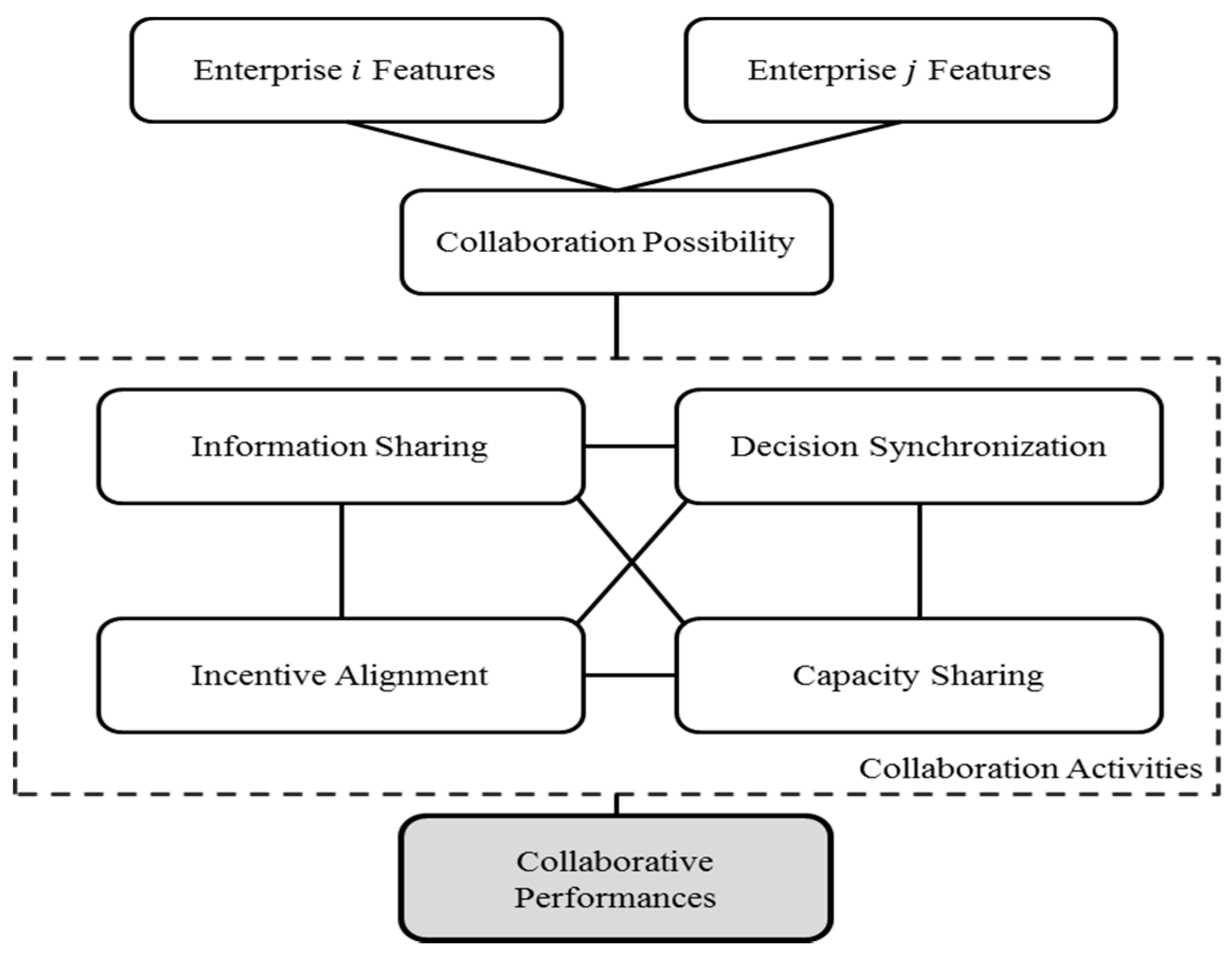
2. Proposed Framework

The proposed framework consists of five steps: (1) defining variables and their relationships; (2) designing a probabilistic graphical model; (3) collecting data; (4) learning the probabilistic graphical model; and (5) estimating the collaboration level. Each step is explained in detail in the following subsections. The proposed framework in this research can be used to estimate collaboration level between entities in the supply chain such as supplier of raw material, part manufacturer, and logistic company. Namely, participating enterprises i and j in Figure 1 can be regarded as the supply chain entities.

2.1. Defining Variables and Their Relationships

From the literature reviews, we consider enterprise features, collaboration possibility, collaboration activities, and collaborative performances as dimensions which compose the graph. Figure 1 shows the relationships between these dimensions. Note that the dimensions can be modified according to a user’s objectives. For example, one may not use capacity sharing to find the collaboration level.

Variables in the enterprise feature dimension are defined by referring to literature which introduces service provider models in CM. Wang and Xu [41] developed a service provider model in CM, which expresses an enterprise as provider ID, company name, provider size, provider capability, provider location, provider evaluation, retaining resources, and so forth. In MFG.com [42], which is one of the most promising CM companies, the service provider (enterprise) is expressed as: general description, products, industries, customer manufacturing services, location, and rating. Among these variables, we select three variables to compose an enterprise features dimension as follows: service type, manufacturing resources, and geographical location. Only three variables are selected because these are sufficient to explain the enterprise feature dimension as they can include other variables and these variables impact the collaboration.

As seen in Figure 1, the features of two enterprises directly impact their collaboration potentiality. To be more concrete, two enterprises located near each other would collaborate more efficiently than two enterprises located far from each other. In addition, both enterprises which provide manufacturing services that can be interchangeable or composed of each other’s products would be more likely to collaborate with each other. Accordingly, the collaboration possibility dimension includes two variables: geographical distance and possible service interchangeability and composition.

From the literature reviews regarding the collaborative supply chain, whose environment is similar to the CM environment, we define variables belonging to the collaboration activities dimensions (i.e., information sharing, decision synchronization, incentive alignment, and capacity sharing). Information sharing refers to the ability to see private data in a partner’s systems and monitor the production process in the supply chain through communication [43]. Information sharing has been measured using several factors such as inventory level information sharing [31,34,43,44,45,46,47], collaborative demand forecasting [31,44,45,46], new product development plan sharing [31,35,45,48,49], manufacturing schedule sharing [35,44,48,49,50], and manufacturing ability sharing [44,45,48,50]. Decision synchronization is defined as the ability to synchronize decisions at different managerial levels to pursue the common goal of optimizing supply chain profitability between enterprises [43]. This dimension has been measured by several factors such as operational decisions [31,43,49,51,52], strategic decisions [31,35,49,51,52], and policy decisions [34,43]. Operational decisions include decisions on inventory requirements, optimal order quantity and purchasing, etc. Strategic decisions include decisions regarding the development of new products, joint plans on promotional events, etc. [43]. Policy decisions include pricing and payment policy [34]. Incentive alignment refers to the process of sharing costs, risks, and benefits amongst the participating members [43]. Incentive alignment means sharing cost [43], benefits [53], and risk [53,54] among enterprises in a supply chain. Capacity sharing refers to the joint use of manufacturing resources such as warehouses, labor, and equipment [55]. Capacity sharing has been measured as manufacturing equipment sharing [25,41,49,55], storage sharing [25,35,41,49], technology sharing [25,35,41,49], and personal sharing [41].

Finally, we establish collaborative performance factors referring to research and a CM company (MFG.com). These factors are project ratings which include the customer evaluation for a manufacturing service production [42], quality improvement [33,42,56], total cost reduction [33,45,49,56], lead time reduction [33,45,49], and resource utilization improvement [45].

Table 1. Overall variables used in this paper.

Dimension	Variable	Explanation	Values	References
Enterprise Features	$S{T}_i$	Service type enterprise i provides	p: Type p service (p =1,2,3,4)	[2,42]
	$M{R}_i$	Manufacturing resources of enterprise i	q: Type resource q (q = 1,2,3,4)	[2,42]
	$G{L}_i$	Geographical location of enterprise i	r: Region (r = 1,2,3)	[2,42]
Collaboration Possibility	$I{C}_{i,j}$	Interchangeability and composability of services enterprises i and j provide	1: Interchangeable or composable 0: Otherwise	-
	$G{D}_{i,j}$	Geographical distance between enterprises i and j	1: They are closely located 0: Otherwise	-
Information Sharing	$I{L}_{i,j}$	Inventory level sharing between enterprises i and j	1: They have shared inventory level 0: Otherwise	[31,34,43,44,45,46,47,50]
	$D{F}_{i,j}$	Collaborative demand forecasting between enterprises i and j	1: They have collaboratively forecasted demand 0: Otherwise	[31,44,45,46]
	$N{P}_{i,j}$	New product development plan sharing between enterprises i and j	1: They have shared new product development plan 0: Otherwise	[31,35,45,48,49]
	$M{S}_{i,j}$	Manufacturing schedule sharing between enterprises i and j	1: They have shared manufacturing schedules 0: Otherwise	[35,44,48,49,50]
	$M{A}_{i,j}$	Information of manufacturing ability sharing between enterprises i and j	1: They have shared manufacturing ability 0: Otherwise	[44,45,48,50]
Decision Synchronization	$O{D}_{i,j}$	Operational decision synchronization between enterprises i and j	1: They have collaboratively made a decision regarding operational issues 0: Otherwise	[31,43,49,51,52]
	$S{D}_{i,j}$	Strategic decision synchronization between enterprises i and j	1: They have collaboratively made a decision regarding strategic issues 0: Otherwise	[31,35,49,51,52]
	$P{D}_{i,j}$	Policy decision synchronization between enterprises i and j	1: They have collaboratively made a decision regarding policy issues 0: Otherwise	[34,43]
Incentive Alignment	$C{S}_{i,j}$	Cost sharing between enterprises i and j	1: They have shared cost 0: Otherwise	[3]
	$B{S}_{i,j}$	Benefit sharing between enterprises i and j	1: They have shared benefit 0: Otherwise	[53]
	$R{S}_{i,j}$	Risk sharing between enterprises i and j	1: They have shared risk 0: Otherwise	[53,54]
Capacity Sharing	$M{E}_{i,j}$	Manufacturing equipment sharing between enterprises i and j	1: They have shared manufacturing equipment 0: Otherwise	[25,35,41,49]
	$S{O}_{i,j}$	Storage sharing between enterprise $si$ and $j$	1: They have shared storage 0: Otherwise	[25,35,41,49]
	$T{E}_{i,j}$	Technology sharing between enterprises $i$ and $j$	1: They have shared technology 0: Otherwise	[25,35,41,49]
	$P{E}_{i,j}$	Personnel sharing between enterprises $i$ and $j$	1: They have shared personnel 0: Otherwise	[41]
Collaborative Performance	$Q{U}_{i,j}$	Quality improvement of both enterprises $i$ and $j$	1: They have experienced quality improvement through collaboration 0: Otherwise	[33,42,56]
	$T{C}_{i,j}$	Total cost reduction of both enterprises $i$ and $j$	1: They have experienced total cost reduction through collaboration 0: Otherwise	[33,45,49,56]
	$R{U}_{i,j}$	Resource utilization improvement of both enterprises $i$ and $j$	1: They have experienced resource utilization improvement through collaboration 0: Otherwise	[45]

summarizes all the variables used in this paper. Note that practitioners could modify the variables according to their own objectives. For instance, we assumed that every variable in all dimensions, except for enterprise features, is a binary type, but practitioners can change some variables to those measured by a 5 point Likert scale. In addition, dimensions or variables can be added or eliminated.

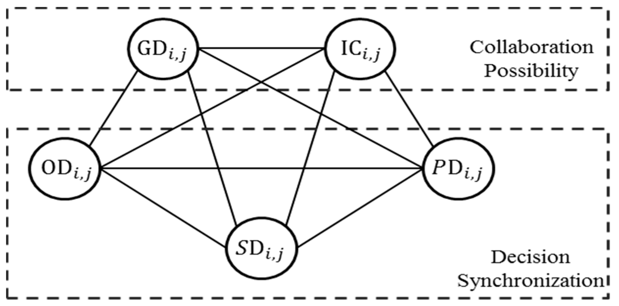
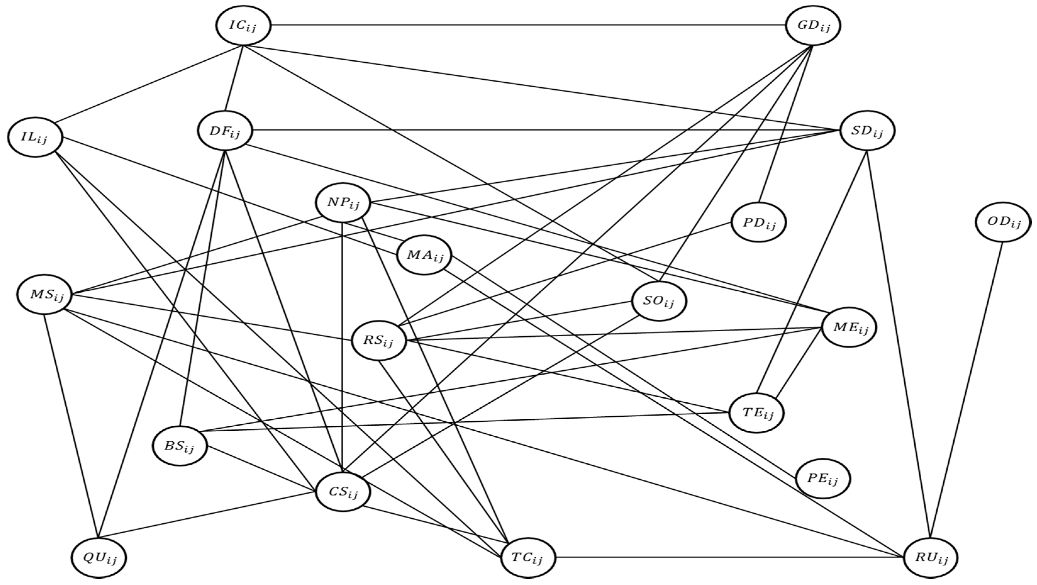
2.2. Designing the Probabilistic Graphical Model

Designing the PGM consists of two steps, namely (1) designing a graph structure; and (2) designing potential functions. The first step includes determining a graph type and connecting some nodes by edges. Note that each variable is mapped as a corresponding node, which imposes that there is no need to define the nodes. The second step is to design mathematical functions (potential functions) that compose the PGM.

Either a directed or undirected graph can be used as the graph type. In general, the former is employed to express conditional relationships among variables while the latter is employed to express correlation among the variables. Since correlations among the variables in Table 1 may exist, we adopt a Markov random field (MRF), which is one of the most used undirected graphs. The remaining task is to connect nodes by edges. Since there is no previous research which verifies the relationships among the variables, we cannot use proper domain knowledge to connect the nodes in the graph. We construct an initial graph and modify the initial graph based on the structure learning result. In the initial graph, every node in the same dimensions is connected with edges, and every node in two connected dimensions is also connected. For example, Figure 2 shows a part of the initial graph. As seen in Figure 2, there is a connection between $G{D}_{i,j}$ and $I{C}_{i,j}$ which are in the same dimension (i.e., collaboration possibility). $G{D}_{i,j}$ and $O{D}_{i,j}$ are also connected because $G{D}_{i,j}$ and $O{D}_{i,j}$ are included in collaboration possibility and decision synchronization, which are connected dimensions, respectively. The initial graph includes 184 edges.

We design two kinds of potential functions. The first ones are to eliminate the edges in the initial graph, and each function is assigned to the corresponding edge. The second ones are to find the joint probabilities which are based on estimate collaboration levels in CM, and each function is assigned to the corresponding cliques. We present the method to modify the initial graph structure in Section 2.4, and the method to find the joint probabilities in Section 2.5.

The potential functions can be freely designed, and we provide two examples of these. The first example is a potential function assigned to an edge, which reflects our assumption that if enterprises $i$ and $j$ share manufacturing equipment then they may share related technology. The function is presented in Equation (1),

$$\varphi \left(M{E}_{i,j}, T{E}_{i,j}\right)=\{\begin{array}{cc}2,& if M{E}_{i,j}=T{E}_{i,j}=1\\ 1,& if M{E}_{i,j}=T{E}_{i,j}=0\\ 0,& otherwise\end{array}$$

(1)

where $\varphi \left(\cdot \right)$ denotes the potential function. The values $\varphi \left(M{E}_{i,j}, T{E}_{i,j}\right)$ can be freely defined, since the weight assigned to the function adjusts these values. It is desirable, however, to make a potential function have a larger value when it satisfies an assumption. Note that the assumption used in Equation (1) is that if enterprises $i$ and $j$ share manufacturing equipment then they may share related technology. As the second example, let’s assume that $C{S}_{i,j}$, $B{S}_{i,j}$ and $R{S}_{i,j}$ form a clique after the structure learning. Then the potential function can be established as follows:

$$\varphi \left(C{S}_{i,j}, B{S}_{i,j}, R{S}_{i,j}\right)=\{\begin{array}{c}\begin{array}{cc}3,& if C{S}_{i,j}=B{S}_{i,j}=R{S}_{i,j}=1\\ 2,& if C{S}_{i,j}=B{S}_{i,j}=R{S}_{i,j}=0\end{array}\\ \begin{array}{cc}1,& if C{S}_{i,j}+B{S}_{i,j}+R{S}_{i,j}=2\\ 0,& otherwise\end{array}\end{array}$$

(2)

Note that variables in collaboration possibility of two enterprises are automatically determined according to the values of variables in the enterprises features. In other words, there is no reason to employ potential functions to express relationships between variables in collaboration possibility and enterprise features. We assume the following relations:

$$\mathrm{IF} S{T}_i=S{T}_j and M{R}_i=M{R}_j \mathrm{THEN} I{C}_{i,j}=1, \mathrm{OTHERWISE} I{C}_{i,j}=0$$

(3)

$$\mathrm{IF} G{L}_i=G{L}_j \mathrm{THEN} G{D}_{i,j}=1, \mathrm{OTHERWISE} G{D}_{i,j}=0.$$

(4)

2.3. Collecting Data

The third step is to collect data using a survey. We do not develop whole questionnaire but we provide example questions which may be referenced as follows:

• Q. Which type of manufacturing service does your company provide?
  (1) Assembly (2) Machining (3) Molding (4) Fabrication (5) Prototyping
• Q. Specify the company names that your company has collaborations with.
  (   )
• Q. How much has your company shared inventory with “Company A”?
  (1) Never (2) Rarely (3) Sometimes (4) Often (5) Always
• Q. How much has your quality improved through collaboration with “Company B”?
  (1) Never (2) Little (3) Somewhat (4) Much (5) A Great Deal

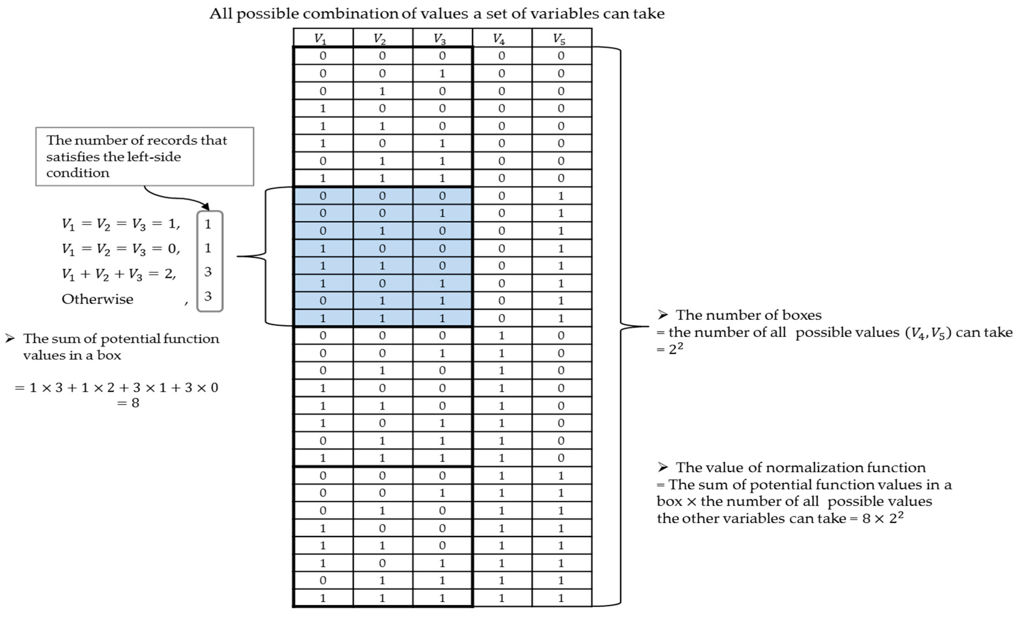
2.4. Learning Probabilistic Graphical Model

Learning tasks are divided into two parts, namely (1) to estimate a weight assigned to each edge, and (2) to estimate a weight assigned to each clique. As mentioned before, the first and second tasks are necessary for structure learning and estimating the collaboration level in CM, respectively. This subsection describes both learning methods based on the maximum likelihood estimation (MLE).

Let $e$ be an edge in the graph, and let $d$ be a pair of two companies that collaborate with each other in a dataset, $\mathit{D}$. The dataset size is $M$, which represents the number of pairs in the dataset. Given a set of weights, $\mathit{w}$, the log likelihood is calculated as follows [57]:

$$\log \mathrm{P}\left(\mathit{w}|\mathit{D}\right)={\displaystyle \sum }_d\left\{{\displaystyle \sum }_e\log \left(w_e\varphi \left(e;d\right)\right)\right\}-M\log Z\left(G{D}_{i,j}, I{C}_{i,j}, \dots , T{C}_{i,j}, R{U}_{i,j}\right),$$

(5)

where $w_e$ and $\varphi \left(e;d\right)$ indicate the weight assigned to $e$, and the value of the potential function for $e$ when data $d$ is entered, respectively. $Z\left(G{D}_{i,j}, I{C}_{i,j}, \dots , T{C}_{i,j}, R{U}_{i,j}\right)$ denotes a normalization function calculated as follows (we will explain the normalization function in Section 2.5):

$$Z\left(G{D}_{i,j}, I{C}_{i,j}, \dots , T{C}_{i,j}, R{U}_{i,j}\right)={\displaystyle \sum }_{G{D}_{i,j}}{\displaystyle \sum }_{I{C}_{i,j}}\cdots {\displaystyle \sum }_{R{U}_{i,j}}\left({\displaystyle \sum }_{k=1}^K{w}_k\varphi \left({\mathrm{C}}_k\right)\right).$$

(6)

The estimated set of weights $\widehat{\mathit{w}}$ satisfies following condition:

$$\widehat{\mathit{w}}=\underset{\mathit{w}}{\mathrm{argmax}}\log \mathrm{P}\left(\mathit{w}|\mathit{D}\right).$$

(7)

Because it is almost impossible to find $\widehat{\mathit{w}}$ which satisfies Equation (7) by analytical approach, a meta-heuristic method such as a genetic algorithm is usually adopted. We adopt a genetic algorithm in this paper. For simplicity, we assume the range of each weight is [0, 1]. After the estimation, if an estimated weight for an edge $e$, ${\widehat{w}}_e$ is smaller than a threshold, then we eliminate the edge from the graph. Note that the threshold is a user parameter, and if the threshold is set as high then the graph would be sparse. Otherwise, the graph would be dense.

Let $c$ be a clique after the graph structure is defined. Similar to Equation (5), the log likelihood is calculated as follows:

$$\log \mathrm{P}\left(\mathit{w}|\mathit{D}\right)={\displaystyle \sum }_d\left\{{\displaystyle \sum }_c\log \left(w_c\varphi \left(c;d\right)\right)\right\}-M\log Z\left(G{D}_{i,j}, I{C}_{i,j}, \dots , T{C}_{i,j}, R{U}_{i,j}\right),$$

(8)

where $w_c$ and $\varphi \left(c;d\right)$ denote the weight assigned to $c$ and the value of the potential function for c when data d is entered, respectively. Note that a potential function for each clique may be newly defined after the structure learning, and the corresponding weights should be estimated as seen in Equation (8).

2.5. Estimating Collaboration Level

A MRF efficiently yields joint probability distribution of all variables as follows [57]:

$$\mathrm{P}\left(\mathit{X}=\mathit{x}\right)=\frac{1}{Z}\exp \left({\displaystyle \sum }_k{\displaystyle \sum }_l{w}_{l,k}{\varphi }_l\left(c_k\right)\right)$$

(9)

where ${\mathit{c}}_k$ is the $k$th clique in the set of all cliques $\mathit{C}$, ${\varphi }_l$ denotes the $l$th potential function, $w_{l,k}$ denotes the weight assigned to the ${\varphi }_l$ for ${\mathit{c}}_k$, and $Z$ is a normalization function that ensures $\mathrm{P}\left(\mathit{X}=\mathit{x}\right)$ a valid probability distribution.

Based on Equation (9), we can estimate the joint probability $\mathrm{P}\left(G{D}_{i,j}, I{C}_{i,j}, \dots , T{C}_{i,j}, R{U}_{i,j}\right)$ as follows:

$$\mathrm{P}\left(G{D}_{i,j}, I{C}_{i,j}, \dots , T{C}_{i,j}, R{U}_{i,j}\right)=\frac{1}{Z\left(G{D}_{i,j}, I{C}_{i,j}, \dots , T{C}_{i,j}, R{U}_{i,j}\right)}{\displaystyle \sum }_{k=1}^K{w}_k\varphi \left({\mathrm{C}}_k\right),$$

(10)

where $K$ indicates the number of cliques included in the graph structure, and $C_k$ denotes clique $k$.

Marginalizing Equation (10), we can calculate the conditional probabilities that variables have 1 in the collaborative performance dimension given collaborative performance factors such as $\mathrm{P}\left(Q{U}_{i,j}=1|G{D}_{i,j}, I{C}_{i,j}, \dots ,P{E}_{i,j}\right)$, $\mathrm{P}\left(T{C}_{i,j}=R{U}_{i,j} =1|G{D}_{i,j}, I{C}_{i,j}, \dots ,P{E}_{i,j}\right)$, and $\mathrm{P}\left(Q{U}_{i,j}=T{C}_{i,j}=R{U}_{i,j}=1|G{D}_{i,j}, I{C}_{i,j}, \dots ,P{E}_{i,j}\right)$. We call these conditional probabilities the collaboration levels between two enterprises in CM. As an example of the probability calculation, $\mathrm{P}\left(T{C}_{i,j}=R{U}_{i,j} =1|G{D}_{i,j}, I{C}_{i,j}, \dots ,P{E}_{i,j}\right)$ is calculated as follows:

$$\mathrm{P}\left(Q{U}_{i,j}=T{C}_{i,j}={\mathrm{RU}}_{i,j}=1|G{D}_{i,j}, I{C}_{i,j}, \dots ,P{E}_{i,j}\right)=\frac{\mathrm{P}\left(G{D}_{i,j}, I{C}_{i,j}, \dots , P{E}_{i,j}, Q{U}_{i,j}=1, T{C}_{i,j}=1,{\mathrm{RU}}_{i,j}= 1\right)}{P\left(G{D}_{i,j}, I{C}_{i,j}, \dots ,P{E}_{i,j}\right)}=\frac{\mathrm{P}\left(G{D}_{i,j}, I{C}_{i,j}, \dots , P{E}_{i,j}, Q{U}_{i,j}=1, T{C}_{i,j}=1,{\mathrm{RU}}_{i,j}=1\right)}{{\displaystyle {\sum }_{Q{U}_{i,j}=0}^1{\displaystyle {\sum }_{T{C}_{i,j}=0}^1{\displaystyle {\sum }_{R{U}_{i,j}=0}^1\mathrm{P}\left(G{D}_{i,j}, I{C}_{i,j}, \dots , T{C}_{i,j}, R{U}_{i,j}\right)}}}}$$

(11)

In addition, we can calculate conditional probabilities by marginalization even though some values are missing. For example, let the values of $M{E}_{i,j}$, $S{O}_{i,j}$, $T{E}_{i,j}$ and $P{E}_{i,j}$ be not given, and we want to calculate the probability that both enterprise $i$ and $j$ will improve resource utilization through collaboration between them, $\mathrm{P}\left(R{U}_{i,j}=1|G{D}_{i,j}, I{C}_{i,j}, \dots ,R{S}_{i,j}\right)$. It can be calculated as follows:

$$\mathrm{P}\left(R{U}_{i,j} =1|G{D}_{i,j}, I{C}_{i,j}, \dots ,R{S}_{i,j}\right)=\frac{\mathrm{P}\left(G{D}_{i,j}, I{C}_{i,j}, \dots ,R{S}_{i,j}, R{U}_{i,j}=1\right)}{\mathrm{P}\left(G{D}_{i,j}, I{C}_{i,j}, \dots ,R{S}_{i,j}\right)}=\frac{{\displaystyle {\sum }_{Q{U}_{i,j}=0}^1{\displaystyle {\sum }_{T{C}_{i,j}=0}^1{\displaystyle {\sum }_{M{E}_{i,j}=0}^1{\displaystyle {\sum }_{S{O}_{i,j}=0}^1{\displaystyle {\sum }_{E_{i,j}=0}^1{\displaystyle {\sum }_{P{E}_{i,j}=0}^1\mathrm{P}}}}\left(G{D}_{i,j}, I{C}_{i,j}, \dots , T{C}_{i,j}, R{U}_{i,j}\right)}}}}{{\displaystyle {\sum }_{Q{U}_{i,j}=0}^1{\displaystyle {\sum }_{T{C}_{i,j}=0}^1{\displaystyle {\sum }_{R{U}_{i,j}=0}^1{\displaystyle {\sum }_{M{E}_{i,j}=0}^1{\displaystyle {\sum }_{S{O}_{i,j}=0}^1{\displaystyle {\sum }_{E_{i,j}=0}^1{\displaystyle {\sum }_{P{E}_{i,j}=0}^1\mathrm{P}}}}\left(G{D}_{i,j}, I{C}_{i,j}, \dots , T{C}_{i,j}, R{U}_{i,j}\right)}}}}}$$

(12)

3. Illustrative Example

In this section, we provide an example to illustrate how to apply the framework in practice. In the example, we assume that 20 enterprises participate in CM and they collaborate with each other. Even though a group of $h\left(3\le h\le 20\right)$ enterprises can have collaboratively produced manufacturing services, we assume the group is partitioned to $\left(\begin{array}{c}h\\ 2\end{array}\right)$ small groups whose size is 2. Namely, the number of pairs of two collaborative companies is $\left(\begin{array}{c}20\\ 2\end{array}\right)=190$.

We generate data from each variable distribution we assumed. First of all, distributions of the variables in the enterprise features dimension are as follows:

$$\mathrm{P}\left(S{T}_i=k\right)=\frac{1}{4},\mathrm{for}i=1,2,\dots ,20,p=1,2,3,4,$$

(13)

$$\mathrm{P}\left(G{L}_i=k\right)=\frac{1}{3},\mathrm{for}i=1,2,\dots ,20,r=1,2,3,$$

(14)

$$\mathrm{P}\left(M{R}_i=k|S{T}_i=k\right)=0.8,\mathrm{P}\left(M{R}_i=q|S{T}_i=k\right)=0.2\times \frac{1}{3},\mathrm{for}k=1,2,3,4,q\ne k.$$

(15)

In addition, we assume the values of factors in dimensions of information sharing, decision synchronization, incentive alignment, and capacity sharing are determined as follows:

$$\mathrm{P}\left(facto{r}_{i,j}=1|I{C}_{i,j}=1, G{D}_{i,j}=1\right)=0.7,\mathrm{for}i=1,2,\dots ,19,i<j$$

(16)

$$\mathrm{P}\left(facto{r}_{i,j}=1|I{C}_{i,j}=1, G{D}_{i,j}=0\right)=0.5,\mathrm{for}i=1,2,\dots ,19,i<j$$

(17)

$$\mathrm{P}\left(facto{r}_{i,j}=1|I{C}_{i,j}=0, G{D}_{i,j}=1\right)=0.5,\mathrm{for}i=1,2,\dots ,19,i<j$$

(18)

$$\mathrm{P}\left(facto{r}_{i,j}=1|I{C}_{i,j}=0, G{D}_{i,j}=0\right)=0.1,\mathrm{for}i=1,2,\dots ,19,i<j$$

(19)

where $facto{r}_{i,j}$ indicates a factor included in these dimensions (e.g., $I{L}_{i,j}$, $T{E}_{i,j}$).

Finally, we assume the values of factors in collaborative performance are determined as follows:

$$\mathrm{P}\left(Q{U}_{i,j}=1|I{L}_{i,j}+D{F}_{i,j}+\dots +P{E}_{i,j}=n\right)=\frac{n}{15},$$

(20)

$$\mathrm{P}\left(T{C}_{i,j}=1|I{L}_{i,j}+D{F}_{i,j}+\dots +P{E}_{i,j}=n\right)=\frac{n}{15},$$

(21)

$$\mathrm{P}\left(R{U}_{i,j}=1|I{L}_{i,j}+D{F}_{i,j}+\dots +P{E}_{i,j}=n\right)=\frac{n}{15}.$$

(22)

We define the potential function for each edge to modify the initial graph. Since all variables, except for the variables in the enterprise features dimension, are binary, we use potential functions in the same form (i.e., 184 potential functions for each edge have the same form) as follows:

$${\varphi }_1\left(V{1}_{i,j}, V{2}_{i,j}\right)=\{\begin{array}{cc}2,& if V{1}_{i,j}=V{2}_{i,j}=1\\ 1,& if V{1}_{i,j}=V{2}_{i,j}=0\\ 0,& otherwise\end{array}$$

(23)

where $V{1}_{i,j}$ and $V{2}_{i,j}$ are the two variables connected by an edge in the initial graph.

We adopt the genetic algorithm to estimate the set of weights assigned to edges, and we eliminate 138 edges whose corresponding weights are smaller than 0.8. From the elimination process, we obtain the graph structure which is given in Figure 3. Note that we omit the dimension of enterprise features in Figure 3, because the potential functions are not assigned to the edges linking the nodes in the dimension as mentioned before.

The graph presented in Figure 3 includes 27 cliques whose size is 2 or 3. For cliques whose size is 2 (i.e., cliques which include two nodes), we employ again the potential functions presented in (23), and we design the clique potential form for the cliques whose size is 3 as follows:

$${\varphi }_2\left(V{1}_{i,j}, V{2}_{i,j}, V{3}_{i,j}\right)=\{\begin{array}{c}\begin{array}{cc}3,& if V{1}_{i,j}=V{2}_{i,j}= V{3}_{i,j}=1\\ 2,& if V{1}_{i,j}=V{2}_{i,j}= V{3}_{i,j}=0\end{array}\\ \begin{array}{cc}1,& if V{1}_{i,j}+V{2}_{i,j}+ V{3}_{i,j}= 2\\ 0,& otherwise\end{array}\end{array}$$

(24)

where $V{1}_{i,j}$, $V{2}_{i,j}$ and $V{3}_{i,j}$ are variables included in the same clique (e.g., $V{1}_{i,j}$, $V{2}_{i,j}$ and $V{3}_{i,j}$ are $I{C}_{i,j}$, $D{F}_{i,j}$, and $S{D}_{i,j}$, respectively).

We also adopt the genetic algorithm to estimate the weight of each potential function, and

Table 2. Clique information and learning result.

Clique	Variables	Weight
${\mathrm{C}}_1$	$I{C}_{i,j}, I{L}_{i,j}$	0.5004
${\mathrm{C}}_2$	$I{C}_{i,j},D{F}_{i,j},S{D}_{i,j}$	0.9768
${\mathrm{C}}_3$	$I{C}_{i,j},S{O}_{i,j}$	0.8985
${\mathrm{C}}_4$	$G{D}_{i,j},P{D}_{i,j},R{S}_{i,j}$	0.7800
${\mathrm{C}}_5$	$G{D}_{i,j},C{S}_{i,j},S{O}_{i,j}$	0.8391
${\mathrm{C}}_6$	$G{D}_{i,j},R{S}_{i,j},S{O}_{i,j}$	0.7346
${\mathrm{C}}_7$	$I{L}_{i,j},M{A}_{i,j}$	0.6401
${\mathrm{C}}_8$	$I{L}_{i,j},C{S}_{i,j},T{C}_{i,j}$	0.8228
${\mathrm{C}}_9$	$D{F}_{i,j},C{S}_{i,j},B{S}_{i,j}$	0.8540
${\mathrm{C}}_{10}$	$D{F}_{i,j},C{S}_{i,j},Q{U}_{i,j}$	0.7149
${\mathrm{C}}_{11}$	$D{F}_{i,j},B{S}_{i,j},M{E}_{i,j}$	0.4255
${\mathrm{C}}_{12}$	$N{P}_{i,j},M{S}_{i,j},S{D}_{i,j}$	0.9206
${\mathrm{C}}_{13}$	$N{P}_{i,j},M{S}_{i,j},T{C}_{i,j}$	0.8757
${\mathrm{C}}_{14}$	$N{P}_{i,j},M{A}_{i,j}$	0.4294
${\mathrm{C}}_{15}$	$N{P}_{i,j},C{S}_{i,j},T{C}_{i,j}$	0.8521
${\mathrm{C}}_{16}$	$N{P}_{i,j},M{E}_{i,j}$	0.8038
${\mathrm{C}}_{17}$	$M{S}_{i,j},S{D}_{i,j},R{U}_{i,j}$	0.9946
${\mathrm{C}}_{18}$	$M{S}_{i,j},R{S}_{i,j},T{C}_{i,j}$	0.1193
${\mathrm{C}}_{19}$	$M{S}_{i,j},Q{U}_{i,j}$	0.8209
${\mathrm{C}}_{20}$	$M{S}_{i,j},T{C}_{i,j},R{U}_{i,j}$	0.5309
${\mathrm{C}}_{21}$	$M{A}_{i,j},P{E}_{i,j}$	0.9671
${\mathrm{C}}_{22}$	$M{A}_{i,j},R{U}_{i,j}$	0.6952
${\mathrm{C}}_{23}$	$O{D}_{i,j},R{U}_{i,j}$	0.2307
${\mathrm{C}}_{24}$	$S{D}_{i,j},T{E}_{i,j}$	0.7174
${\mathrm{C}}_{25}$	$B{S}_{i,j},M{E}_{i,j},T{E}_{i,j}$	0.6907
${\mathrm{C}}_{26}$	$R{S}_{i,j},M{E}_{i,j},T{E}_{i,j}$	0.8250
${\mathrm{C}}_{27}$	$M{E}_{i,j},P{E}_{i,j}$	0.9906

shows the learning result. As seen in Table 2, the graph includes 27 cliques.

We calculate the probabilities presented in Equations (9) and (10) for every combination of two enterprises. For this example, we illustrate the calculation process for the randomly selected combination of enterprises 1 and 17.

Table 3. Values of variables of enterprises 1 and 17.

Variable	Value	Variable	Value	Variable	Value
${\mathrm{IC}}_{i,j}$	0	${\mathrm{OD}}_{i,j}$	0	${\mathrm{SO}}_{i,j}$	0
${\mathrm{GD}}_{i,j}$	1	${\mathrm{SD}}_{i,j}$	0	${\mathrm{TE}}_{i,j}$	1
${\mathrm{IL}}_{i,j}$	1	${\mathrm{PD}}_{i,j}$	1	${\mathrm{PE}}_{i,j}$	1
${\mathrm{DF}}_{i,j}$	1	${\mathrm{CS}}_{i,j}$	0	${\mathrm{QU}}_{i,j}$	1
${\mathrm{NP}}_{i,j}$	1	${\mathrm{BS}}_{i,j}$	0	${\mathrm{TC}}_{i,j}$	0
${\mathrm{MS}}_{i,j}$	0	${\mathrm{RS}}_{i,j}$	1	${\mathrm{RU}}_{i,j}$	1
${\mathrm{MA}}_{i,j}$	1	${\mathrm{ME}}_{i,j}$	1

shows the values of variables of enterprises 1 and 17.

Calculating the joint probability $\mathrm{P}\left(G{D}_{1,17}, I{C}_{1,17}, \dots , T{C}_{1,17}, R{U}_{1,17}\right)$ requires the calculation of the value of the normalization function presented in Equation (6). The value of the normalization function can be practically calculated as follows:

$$\mathrm{Z}\left(G{D}_{i,j},I{C}_{i,j},\dots ,T{C}_{i,j},R{U}_{i,j}\right)=2^{18}\times 4\times {\displaystyle \sum }_{\left|C_k\right|=2}{w}_k{\varphi }_1\left(C_k\right)+2^{17}\times 8\times {\displaystyle \sum }_{\left|C_k\right|=3}{w}_k{\varphi }_2\left(C_k\right),$$

(25)

where ${\displaystyle \sum }_{\left|{\mathrm{C}}_{\mathrm{k}}\right|=3}{w}_k{\varphi }_1\left({\mathrm{C}}_k\right)$ and ${\displaystyle \sum }_{\left|{\mathrm{C}}_{\mathrm{k}}\right|=3}{w}_k{\varphi }_2\left({\mathrm{C}}_k\right)$ denote the weighted sums of potential functions assigned to cliques whose size is 2 and 3, respectively. Figure 4 demonstrates the process by which Equation (25) is derived, with a small example where there are five binary variables and $V_1$, $V_2$ and $V_3$ form a clique. In Figure 4, all possible values that variables in the clique can take are expressed as a box with thick line. The box appears four times and is equal to the number of all possible values that $\left(V_4,V_5\right)$ takes, while the vector is equal to the vector including all variables other than the variables in the clique. In addition, the sum of potential function values when variable values in each box are entered (i.e., ${{\displaystyle \sum }}_{V_1=1}^2{{\displaystyle \sum }}_{V_2=1}^2{{\displaystyle \sum }}_{V_3=1}^1{\varphi }_2\left(V_1,V_2,V_3\right)$) is 8. Thus, the value of the normalization function, which is the sum of potential values when all possible combinations of all the values variables can take, is calculated as follows: ${{\displaystyle \sum }}_{V_1=1}^2{{\displaystyle \sum }}_{V_2=1}^2{{\displaystyle \sum }}_{V_3=1}^1{\varphi }_2\left(V_1,V_2,V_3\right)\times$ number of all possible values of the vector whose elements are remaining variables can take = $2^3\times 4$. In the same way, Equation (24) can be derived. The value of the normalization function in the example with 20 companies is obtained by means of Equation (24), and it is 3914999521.

Based on the values in Table 3 and the normalization function value, $\mathrm{P}\left(G{D}_{1,17}, I{C}_{1,17}, \dots , T{C}_{1,17}, R{U}_{1,17}\right)$ is calculated as follows:

$$\mathrm{P}\left(G{D}_{1,17}, I{C}_{1,17}, \dots , T{C}_{1,17}, R{U}_{1,17}\right)=\frac{1}{\mathrm{Z}\left(G{D}_{1,17}, I{C}_{1,17}, \dots , T{C}_{1,17}, R{U}_{1,17}\right)}{\displaystyle \sum }_{k=1}^K{w}_k{\varphi }_k\left(C_k\right) =\frac{1}{3914999521}\left(0.5004\times 0+0.9768\times 0+0.7800\times 3+\dots +0.9906\times 1\right)=7.22\times {10}^{-9}$$

(26)

Using Equation (25), the various collaboration levels can be calculated and we present each result in Equations (26)–(28).

$$\mathrm{P}\left(Q{U}_{1,17}=1|G{D}_{1,17}, I{C}_{1,17}, \dots ,P{E}_{1,17}\right)=\frac{{\displaystyle {\sum }_{T{C}_{i,j}=0}^1{\sum }_{R{U}_{i,j}=0}^1\mathrm{P}}\left(G{D}_{1,17}, I{C}_{1,17} , \dots , T{C}_{1,17}, R{U}_{1,17}, Q{U}_{1,17}=1\right)}{{\displaystyle {\sum }_{Q{U}_{i,j} = 0}^1{\displaystyle {\sum }_{T{C}_{i,j} = 0}^1{\displaystyle {\sum }_{R{U}_{i,j} = 0}^1\mathrm{P}}}}\left(G{D}_{1,17}, I{C}_{1,17}, \dots , T{C}_{1,17}, R{U}_{1,17}\right)}=\frac{4.49\times {10}^{-9}+4.97\times {10}^{-9}+5.29\times {10}^{-9}+5.37\times {10}^{-9}}{4.04\times {10}^{-8}}=0.4980,$$

(27)

$$\mathrm{P}\left(Q{U}_{1,17}=T{C}_{1,17} =1|G{D}_{1,17}, I{C}_{1,17}, \dots ,P{E}_{1,17}\right)=\frac{{\displaystyle {\sum }_{R{U}_{i,j} = 0}^1\mathrm{P}}\left(G{D}_{1,17}, I{C}_{1,17} , \dots , Q{U}_{1,17}=1, T{C}_{1,17}=1, R{U}_{1,17},\right)}{{\displaystyle {\sum }_{Q{U}_{i,j} = 0}^1{\displaystyle {\sum }_{T{C}_{i,j} = 0}^1{\displaystyle {\sum }_{R{U}_{i,j} = 0}^1\mathrm{P}}}}\left(G{D}_{1,17}, I{C}_{1,17}, \dots , T{C}_{1,17}, R{U}_{1,17}\right)}=\frac{4.49\times {10}^{-9}+4.97\times {10}^{-9}}{4.04\times {10}^{-8}}=0.2342,$$

(28)

$$\mathrm{P}\left(Q{U}_{i,j}=T{C}_{i,j}={\mathrm{RU}}_{i,j}= 1|G{D}_{1,17}, I{C}_{1,17}, \dots ,P{E}_{1,17}\right)=\frac{\mathrm{P}\left(G{D}_{1,17}, I{C}_{1,17} , \dots , Q{U}_{1,17}=1, T{C}_{1,17}=1, R{U}_{1,17}=1\right)}{{\displaystyle {\sum }_{Q{U}_{i,j} = 0}^1{\displaystyle {\sum }_{T{C}_{i,j} = 0}^1{\displaystyle {\sum }_{R{U}_{i,j} = 0}^1\mathrm{P}}}}\left(G{D}_{1,17}, I{C}_{1,17}, \dots , T{C}_{1,17}, R{U}_{1,17}\right)}=\frac{4.49\times {10}^{-9}}{4.04\times {10}^{-8}}=\mathrm{0.11.}$$

(29)

Figure 5 visualizes the calculation results of the conditional probabilities, $\mathrm{P}\left(Q{U}_{i,j}=T{C}_{i,j}=R{U}_{i,j}=1|G{D}_{i,j}, I{C}_{i,j}, \dots ,P{E}_{i,j}\right)$ for all $i$ and $(i<j,i=1,2,\dots ,19,j=1,2,\dots ,20)$. For instance, $\mathrm{P}\left(Q{U}_{1,2}=T{C}_{1,2}=R{U}_{1,2}=1|G{D}_{1,2}, I{C}_{1,2}, \dots ,P{E}_{1,2}\right)>0.5$, $0.3<\mathrm{P}\left(Q{U}_{2,3}=T{C}_{2,3}=R{U}_{2,3}=1|G{D}_{2,3}, I{C}_{2,3}, \dots ,P{E}_{2,3}\right)<0.5$, $\mathrm{P}\left(Q{U}_{1,8}=T{C}_{1,8}=R{U}_{1,8}=1|G{D}_{1,8}, I{C}_{1,8}, \dots ,P{E}_{1,8}\right)<0.3$. This information can be practically applied to group enterprises in CM.

4. Conclusions

Enterprises participating in CM collaborate with each other to more efficiently produce highly customized or moderately large manufacturing services which cannot be produced solely by one enterprise. Collaboration is one of main factors which impacts the qualities of products and services, but there has been no previous research developing a method to estimate collaboration level between enterprises in CM. Accordingly, the operation issues such as task allocation in CM cannot be effectively solved, and therefore it is very important to develop a method to estimate collaboration level between enterprises in CM.

In this paper, we proposed a framework based on the PGM for estimating the collaboration level between enterprises in CM. The variables were brought from thorough literature reviews, and we categorized them into enterprise features, collaboration possibility, information sharing, decision synchronization, incentive alignment, capacity sharing, and collaborative performance. The framework efficiently yields various probabilities that two enterprises in CM will collaborate well (i.e., the probability that they will get a high collaborative performance, given other features (e.g., enterprise feature, information sharing)).

The collaboration levels obtained from the proposed framework could be used to resolve diverse operational problems in CM. The collaboration levels, for instance, would be employed as useful criteria to properly allocate tasks in CM. Concretely, the operator in CM would allocate a task to a set of enterprises with high collaboration level, since they can guarantee manufacturing services with high quality and low operational cost.

For further research, we will statistically verify the relationships among the variables with real data to overcome limitations that we had with the artificial data. As another future research project, we will apply the framework to solve task allocation problems in CM. In other words, it will be necessary to formulate a problem that maximizes the sum (or product) of collaboration levels between enterprises assigned to the task, and to develop more efficient algorithms for this type of problem.

References

1. Ehie, I.C.; Olibe, K. The effect of R&D investment on firm value: An examination of US manufacturing and service industries. Int. J. Prod. Econ. 2010, 128, 127–135. [Google Scholar]
2. Váncza, J.; Monostori, L.; Lutters, D.; Kumara, S.R.; Tseng, M.; Valckenaers, P.; van Brussel, H. Cooperative and responsive manufacturing enterprises. CIRP Ann. Manuf. Technol. 2011, 60, 797–820. [Google Scholar] [CrossRef]
3. Simatupang, T.M.; Sridharan, R. The collaborative supply chain. Int. J. Logist. Manag. 2002, 13, 15–30. [Google Scholar] [CrossRef]
4. Camarinha-Matos, L.M. Collaborative networked organizations in manufacturing. IFAC Proc. Volumes 2007, 40, 187–198. [Google Scholar] [CrossRef]
5. Li, B.H.; Zhang, L.; Wang, S.L.; Tao, F.; Cao, J.W.; Jiang, X.D.; Song, X.; Chai, X.D. Cloud manufacturing: A new service-oriented networked manufacturing model. Comput. Integr. Manuf. Syst. 2010, 16, 1–7. [Google Scholar]
6. Jiang, P.; Ding, K. Social manufacturing: A new way to support outsourcing production. In Proceedings of the 2nd International Conference on Innovative Design and Manufacturing, Taipei, Taiwan, 12–14 December 2012.
7. Rao, Y.; Li, P.; Shao, X.; Wu, B.; Li, B. A CORBA-and MAS-based architecture for agile collaborative manufacturing systems. Int. J. Computer Integr. Manuf. 2006, 19, 815–832. [Google Scholar] [CrossRef]
8. Wu, D.; Greer, M.J.; Rosen, D.W.; Schaefer, D. Cloud manufacturing: Drivers, current status, and future trends. In Proceedings of the ASME 2013 International Manufacturing Science and Engineering Conference collocated with the 41st North American Manufacturing Research Conference, San Diego, CA, USA, 15–21 November 2013.
9. Wu, D.; Rosen, D.W.; Wang, L.; Schaefer, D. Cloud-based design and manufacturing: A new paradigm in digital manufacturing and design innovation. Comput. Aided. Des. 2015, 59, 1–14. [Google Scholar] [CrossRef] [Green Version]
10. Bi, Z.M.; Wang, L. Manufacturing paradigm shift towards better sustainability. In Cloud Manufacturing; Springer: London, UK, 2013. [Google Scholar]
11. Xu, X. From cloud computing to cloud manufacturing. Robot. Cim-Int. Manuf. 2012, 28, 75–86. [Google Scholar] [CrossRef]
12. Jassbi, J.; Di Orio, G.; Barata, D.; Barata, J. The impact of cloud manufacturing on supply chain agility. In Proceedings of the 12th IEEE International Conference on Industrial Informatics, Porto Alegre RS, Brazil, 27–30 July 2014.
13. Singh, A.; Mishra, N.; Ali, S.I.; Shukla, N.; Shankar, R. Cloud computing technology: Reducing carbon footprint in beef supply chain. Int. J. Prod. Econ. 2015, 164, 462–471. [Google Scholar] [CrossRef]
14. Ren, L.; Zhang, L.; Tao, F.; Zhao, C.; Chai, X.; Zhao, X. Cloud manufacturing: from concept to practice. Enterp. Inf. Syst. 2015, 9, 186–209. [Google Scholar] [CrossRef]
15. Xing, K.; Qian, W.; Zaman, A.U. Development of a cloud-based platform for footprint assessment in green supply chain management. J. Clean. Prod. 2016, 139, 191–203. [Google Scholar] [CrossRef]
16. Golightly, D.; Sharples, S.; Patel, H.; Ratchev, S. Manufacturing in the cloud: A human factors perspective. Int. J. Ind. Ergonom. 2016, 55, 12–21. [Google Scholar] [CrossRef]
17. Ren, L.; Cui, J.; Wei, Y.; Laili, Y.; Zhang, L. Research on the impact of service provider cooperative relationship on cloud manufacturing platform. Int. J. Adv. Manuf. Technol. 2016, 86, 2279–2290. [Google Scholar] [CrossRef]
18. Argoneto, P.; Renna, P. Supporting capacity sharing in the cloud manufacturing environment based on game theory and fuzzy logic. Enterp. Inf.Syst. 2016, 10, 193–210. [Google Scholar] [CrossRef]
19. Ahn, G.; Park, Y.J.; Hur, S. The Dynamic Enterprise Network Composition Algorithm for Efficient Operation in Cloud Manufacturing. Sustainability 2016, 8, 1239. [Google Scholar] [CrossRef]
20. Liu, Y.; Zhang, L.; Tao, F.; Wang, L. Resource service sharing in cloud manufacturing based on the Gale–Shapley algorithm: Advantages and challenge. Int. J. Computer Integr. Manuf. 2015. [Google Scholar] [CrossRef]
21. Li, W.; Zhu, C.; Ngai, E.C.H.; Yang, L.T.; Shu, L.; Sheng, Y. Facilities collaboration in cloud manufacturing based on generalized collaboration network. In Proceedings of the 2015 11th International Conference on Heterogeneous Networking for Quality, Reliability, Security and Robustness, Taipei, Taiwan, 19–20 August 2015.
22. Cheng, Z.; Zhan, D.; Zhao, X.; Wan, H. Multitask oriented virtual resource integration and optimal scheduling in cloud manufacturing. J. Appl. Math. 2014. [Google Scholar] [CrossRef]
23. Ming, Y.; Grabot, B.; Houé, R. A typology of the situations of cooperation in supply chains. Comput. Ind. Eng. 2014, 67, 56–71. [Google Scholar] [CrossRef] [Green Version]
24. Ding, H.; Zhao, Q.; An, Z.; Tang, O. Collaborative mechanism of a sustainable supply chain with environmental constraints and carbon caps. Int. J. Prod. Econ. 2016, 181, 191–207. [Google Scholar] [CrossRef]
25. Min, S.; Roath, A.S.; Daugherty, P.J.; Genchev, S.E.; Chen, H.; Arndt, A.D.; Glenn Richey, R. Supply chain collaboration: What’s happening? Int. J. Logist. Manag. 2005, 16, 237–256. [Google Scholar] [CrossRef]
26. Acharya, U.R.; Fujita, H.; Sudarshan, V.K.; Mookiah, M.R.K.; Koh, J.E.; Tan, J.H.; Hagiwara, Y.; Chua, C.K.; Junnarkar, S.M.; Vijayananthan, A.; et al. An integrated index for identification of fatty liver disease using radon transform and discrete cosine transform features in ultrasound images. Inform. Fusion. 2016, 31, 43–53. [Google Scholar] [CrossRef]
27. Barratt, M. Understanding the meaning of collaboration in the supply chain. Supply Chain Manag. 2004, 9, 30–42. [Google Scholar] [CrossRef]
28. Khan, M.; Hussain, M.; Saber, H.M. Information sharing in a sustainable supply chain. Int. J. Prod. Econ. 2016, 181, 208–214. [Google Scholar] [CrossRef]
29. Bian, W.; Shang, J.; Zhang, J. Two-way information sharing under supply chain competition. Int. J. Prod. Econ. 2016, 178, 82–94. [Google Scholar] [CrossRef]
30. Galbreth, M.R.; Kurtuluş, M.; Shor, M. How collaborative forecasting can reduce forecast accuracy. Oper. Res. Lett. 2015, 43, 349–353. [Google Scholar] [CrossRef]
31. Wiengarten, F.; Humphreys, P.; Cao, G.; Fynes, B.; McKittrick, A. Collaborative supply chain practices and performance: Exploring the key role of information quality. Supply Chain Manag. 2010, 15, 463–473. [Google Scholar] [CrossRef]
32. Seok, H.; Nof, S.Y. Collaborative capacity sharing among manufacturers on the same supply network horizontal layer for sustainable and balanced returns. Int. J. Prod. Res. 2014, 52, 1622–1643. [Google Scholar] [CrossRef]
33. Anbanandam, R.; Banwet, D.K.; Shankar, R. Evaluation of supply chain collaboration: A case of apparel retail industry in India. Int. J. Prod. Perf. Manag. 2011, 60, 82–98. [Google Scholar] [CrossRef]
34. Rota, C.; Pugliese, P.; Hashem, S.; Zanasi, C. Assessing the level of collaboration in the Egyptian organic and fair trade cotton chain. J. Clean. Prod. 2016. [Google Scholar] [CrossRef]
35. Ramanathan, U.; Gunasekaran, A.; Subramanian, N. Supply chain collaboration performance metrics: A conceptual framework. Benchmarking Int. J. 2011, 18, 856–872. [Google Scholar] [CrossRef]
36. Inaam, Z.; Abderrahman, M.; Yasmina, H. A framework of Performance Assessment of Collaborative Supply Chain. IFAC-PapersOnLine 2016, 49, 845–850. [Google Scholar] [CrossRef]
37. Koller, D.; Friedman, N. Probabilistic Graphical Models: Principles and Techniques; MIT Press: Cambridge, MA, USA, 2009. [Google Scholar]
38. Jordan, M.I. An introduction to graphical models. Unpublished work. 1997. [Google Scholar]
39. Van der Biest, K.; D’Hondt, R.; Jacobs, S.; Landuyt, D.; Staes, J.; Goethals, P.; Meire, P. EBI: An index for delivery of ecosystem service bundles. Ecol. Indic. 2014, 37, 252–265. [Google Scholar] [CrossRef]
40. Ahn, G.; Hur, H. Continuous Conditional Random Field Model for Predicting the Electrical Load of a Combined Cycle Power Plant. Ind. Eng. Manag. Syst. 2016, 15, 148–155. [Google Scholar] [CrossRef]
41. Wang, X.V.; Xu, X.W. An interoperable solution for Cloud manufacturing. Rob. Comput. Integr. Manuf. 2013, 29, 232–247. [Google Scholar] [CrossRef]
42. MFG.com. Available online: http://www.mfg.com (accessed on 17 November 2016).
43. Simatupang, T.M.; Wright, A.C.; Sridharan, R. The knowledge of coordination for supply chain integration. Bus. Process Manag. J. 2002, 8, 289–308. [Google Scholar] [CrossRef]
44. Baihaqi, I.; Sohal, A.S. The impact of information sharing in supply chains on organisational performance: An empirical study. Prod. Plan. Control 2013, 24, 743–758. [Google Scholar] [CrossRef]
45. Lotfi, Z.; Mukhtar, M.; Sahran, S.; Zadeh, A.T. Information sharing in supply chain management. Procedia Technol. 2013, 11, 298–304. [Google Scholar] [CrossRef]
46. Sari, K. Investigating the value of reducing errors in inventory information from a supply chain perspective. Kybernetes 2015, 44, 176–185. [Google Scholar] [CrossRef]
47. Wu, L.; Chuang, C.H.; Hsu, C.H. Information sharing and collaborative behaviors in enabling supply chain performance: A social exchange perspective. Int. J. Prod. Econ. 2014, 148, 122–132. [Google Scholar] [CrossRef]
48. Barratt, M.; Barratt, R. Exploring internal and external supply chain linkages: Evidence from the field. J. Oper. Manag. 2011, 29, 514–528. [Google Scholar] [CrossRef]
49. Kumar, G.; Nath Banerjee, R. Supply chain collaboration index: An instrument to measure the depth of collaboration. Benchmarking Int. J. 2014, 21, 184–204. [Google Scholar] [CrossRef]
50. Bruque-Cámara, S.; Moyano-Fuentes, J.; Maqueira-Marín, J.M. Supply chain integration through community cloud: Effects on operational performance. J. Purch. Supply Manag. 2016, 22, 141–153. [Google Scholar] [CrossRef]
51. Liao, S.H.; Kuo, F.I. The study of relationships between the collaboration for supply chain, supply chain capabilities and firm performance: A case of the Taiwan’s TFT-LCD industry. Int. J. Prod. Econ. 2014, 156, 295–304. [Google Scholar] [CrossRef]
52. Sigala, M. A supply chain management approach for investigating the role of tour operators on sustainable tourism: The case of TUI. J. Clean. Prod. 2008, 16, 1589–1599. [Google Scholar] [CrossRef]
53. Lehoux, N.; D’Amours, S.; Langevin, A. Inter-firm collaborations and supply chain coordination: Review of key elements and case study. Prod. Plan. Control 2014, 25, 858–872. [Google Scholar] [CrossRef]
54. Cachon, G.P. The allocation of inventory risk in a supply chain: Push, pull, and advance-purchase discount contracts. Manag. Sci. 2004, 50, 222–238. [Google Scholar] [CrossRef]
55. Rivera, L.; Sheffi, Y.; Knoppen, D. Logistics clusters: The impact of further agglomeration, training and firm size on collaboration and value added services. Int. J. Prod. Econ. 2016, 179, 285–294. [Google Scholar] [CrossRef]
56. Koufteros, X.A.; Vonderembse, M.A.; Doll, W.J. Examining the competitive capabilities of manufacturing firms. Struct. Equ. Modeling 2002, 9, 256–282. [Google Scholar] [CrossRef]
57. Murphy, K.P. Machine Learning: A Probabilistic Perspective; MIT Press: Cambridge, MA, USA, 2012. [Google Scholar]
Figure 1. Dimensions considered and their relationships.
Sustainability 09 00277 g001
Figure 2. A part of the initial graph: collaboration possibility and decision synchronization.
Sustainability 09 00277 g002
Figure 3. Learned graph structure in the example.
Sustainability 09 00277 g003
Figure 4. Derivation process of the normalization function value.
Sustainability 09 00277 g004
Figure 5. Calculation results of the collaboration levels.
Sustainability 09 00277 g005