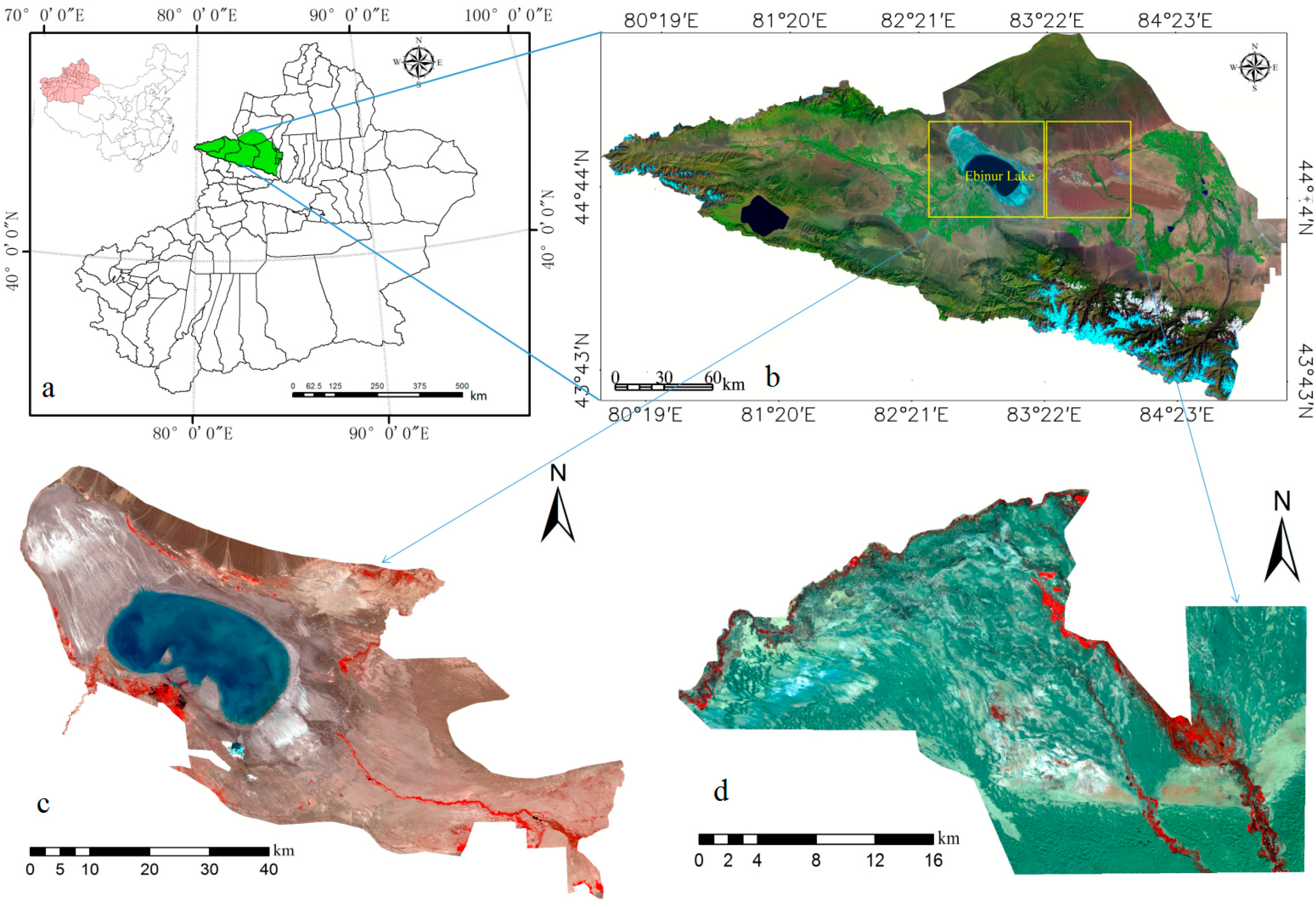
Figure 1.
Location maps of the study area: (a) vicinity map showing the location of the study area within Xinjiang and China; (b) map of the Ebinur Lake vicinity; (c) Ebinur Lake Wetland Nature Reserve; (d) Ganjia Lake Haloxylon Forest Nature Reserve.
Figure 1.
Location maps of the study area: (a) vicinity map showing the location of the study area within Xinjiang and China; (b) map of the Ebinur Lake vicinity; (c) Ebinur Lake Wetland Nature Reserve; (d) Ganjia Lake Haloxylon Forest Nature Reserve.
Figure 2.
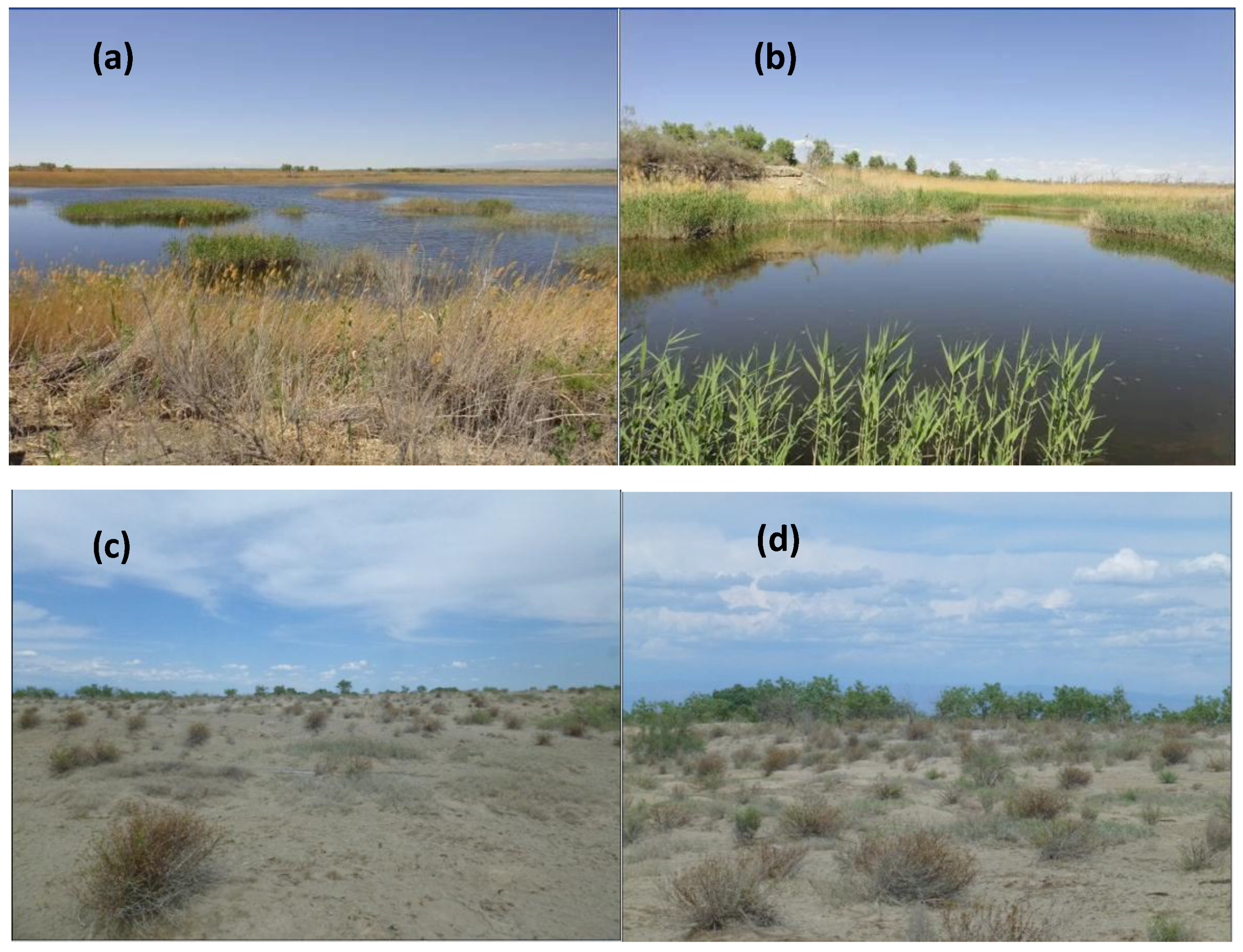
Landscape photos of study area (Photographed by Fei Zhang): (a,b) are Ebinur Lake Wetland National Nature Reserve; (c,d) are Ganjia Lake Haloxylon Forest National Nature Reserve; (a,b) show Ebinur Lake marshes with sparse vegetation. (c,d) show the desert appearance with Haloxylon forest.
Figure 2.
Landscape photos of study area (Photographed by Fei Zhang): (a,b) are Ebinur Lake Wetland National Nature Reserve; (c,d) are Ganjia Lake Haloxylon Forest National Nature Reserve; (a,b) show Ebinur Lake marshes with sparse vegetation. (c,d) show the desert appearance with Haloxylon forest.
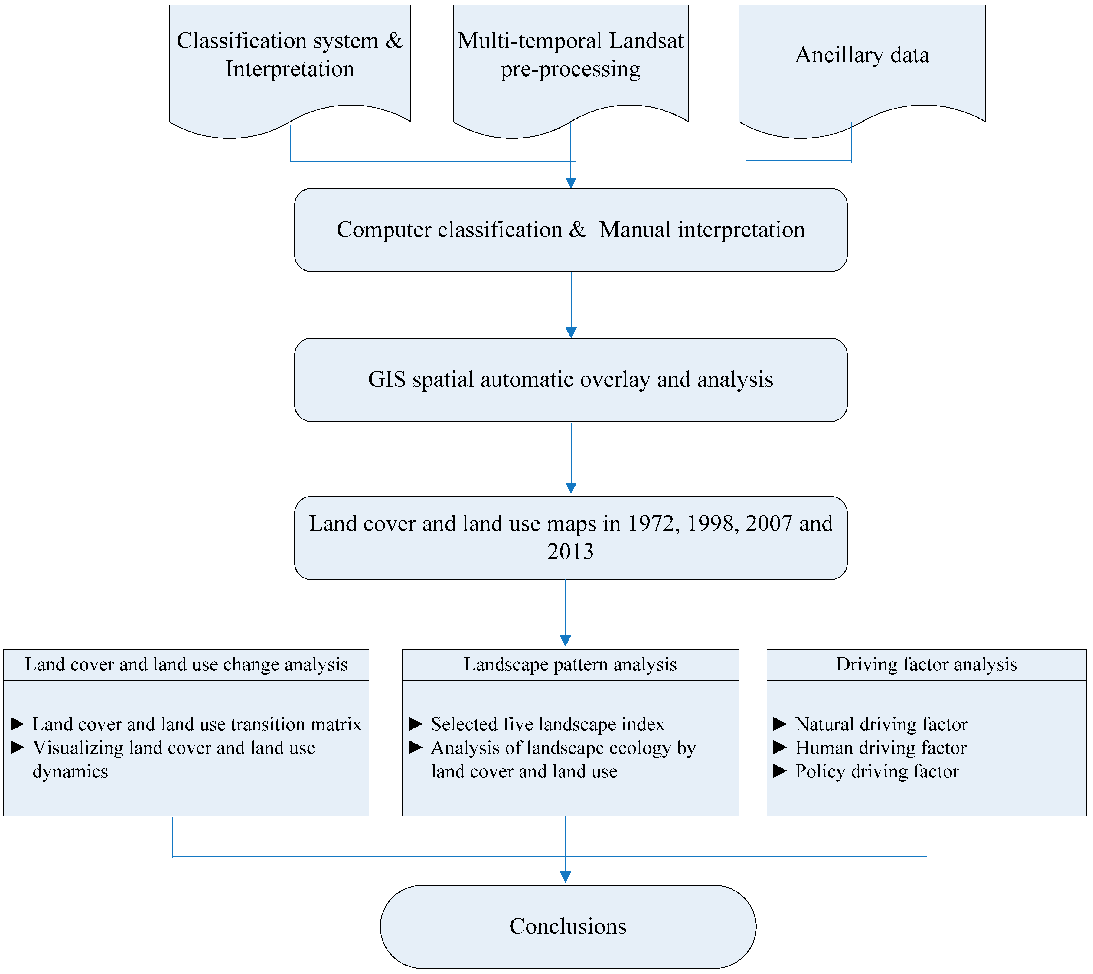
Figure 3.
Flowchart for the land-cover and land-use change and landscape pattern changes in the study area.
Figure 3.
Flowchart for the land-cover and land-use change and landscape pattern changes in the study area.
Figure 4.
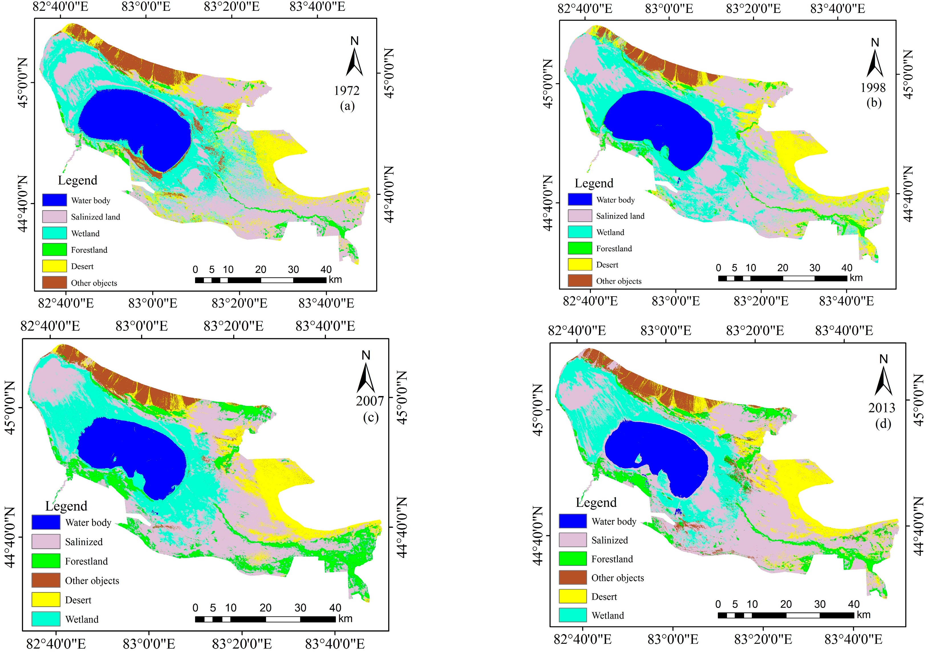
The land cover/land use classification maps in ELWNNR in 1972 (a); 1998 (b); 2007 (c) and 2013 (d).
Figure 4.
The land cover/land use classification maps in ELWNNR in 1972 (a); 1998 (b); 2007 (c) and 2013 (d).
Figure 5.
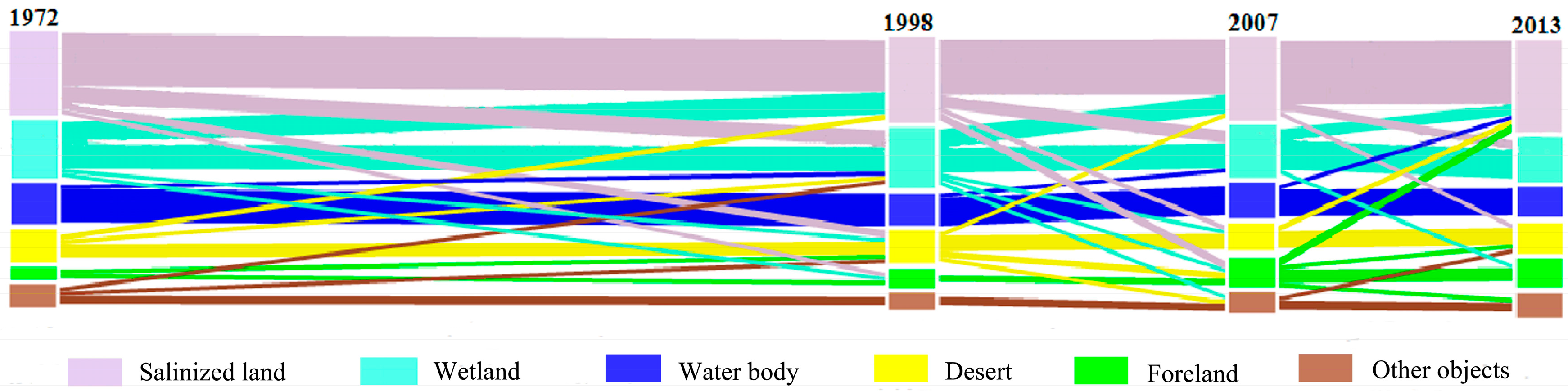
Sankey diagram for comparison of land-cover and land-use dynamics in three time intervals defined by four land cover/use maps from the years 1972, 1998, 2007 and 2013 in the Ebinur Lake National Nature Reserve.
Figure 5.
Sankey diagram for comparison of land-cover and land-use dynamics in three time intervals defined by four land cover/use maps from the years 1972, 1998, 2007 and 2013 in the Ebinur Lake National Nature Reserve.
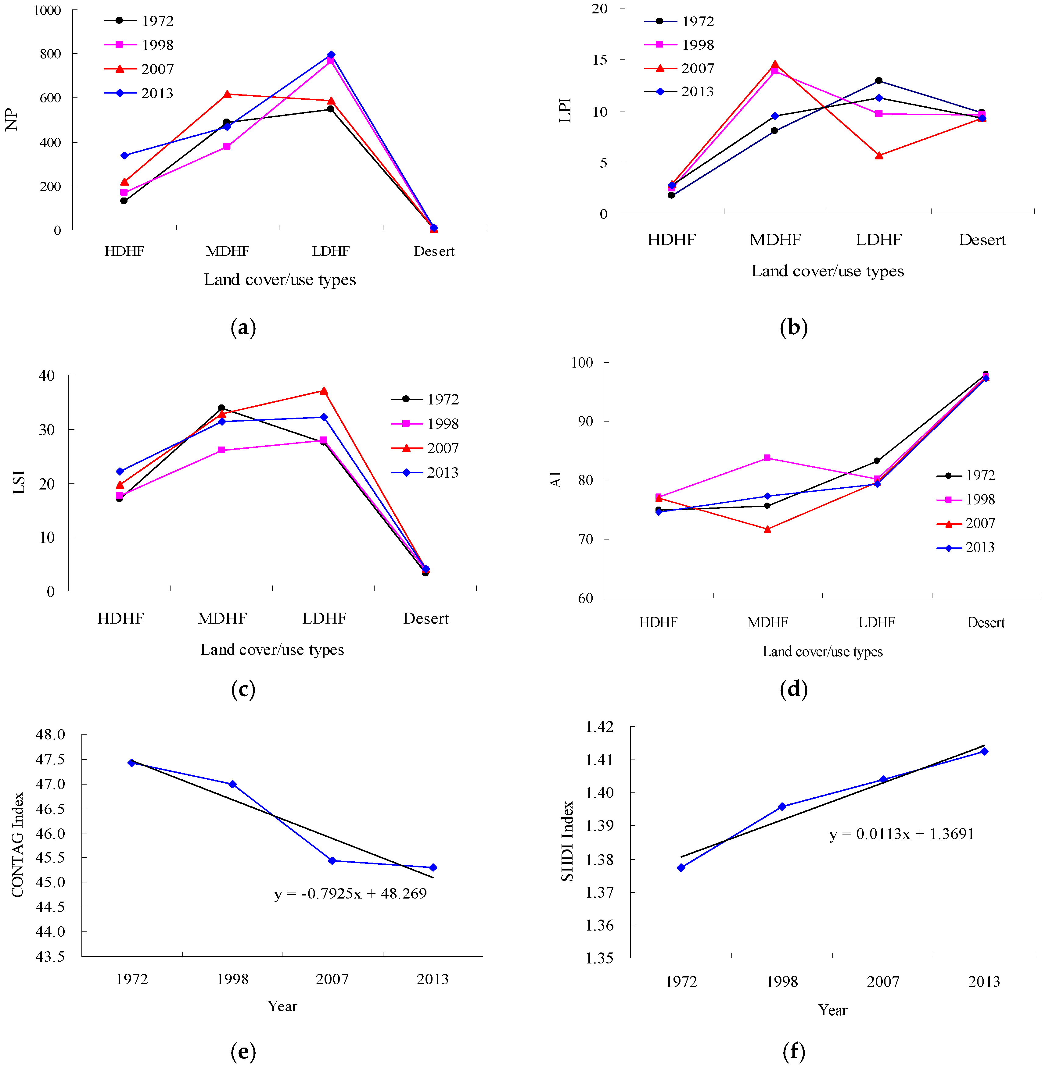
Figure 6.
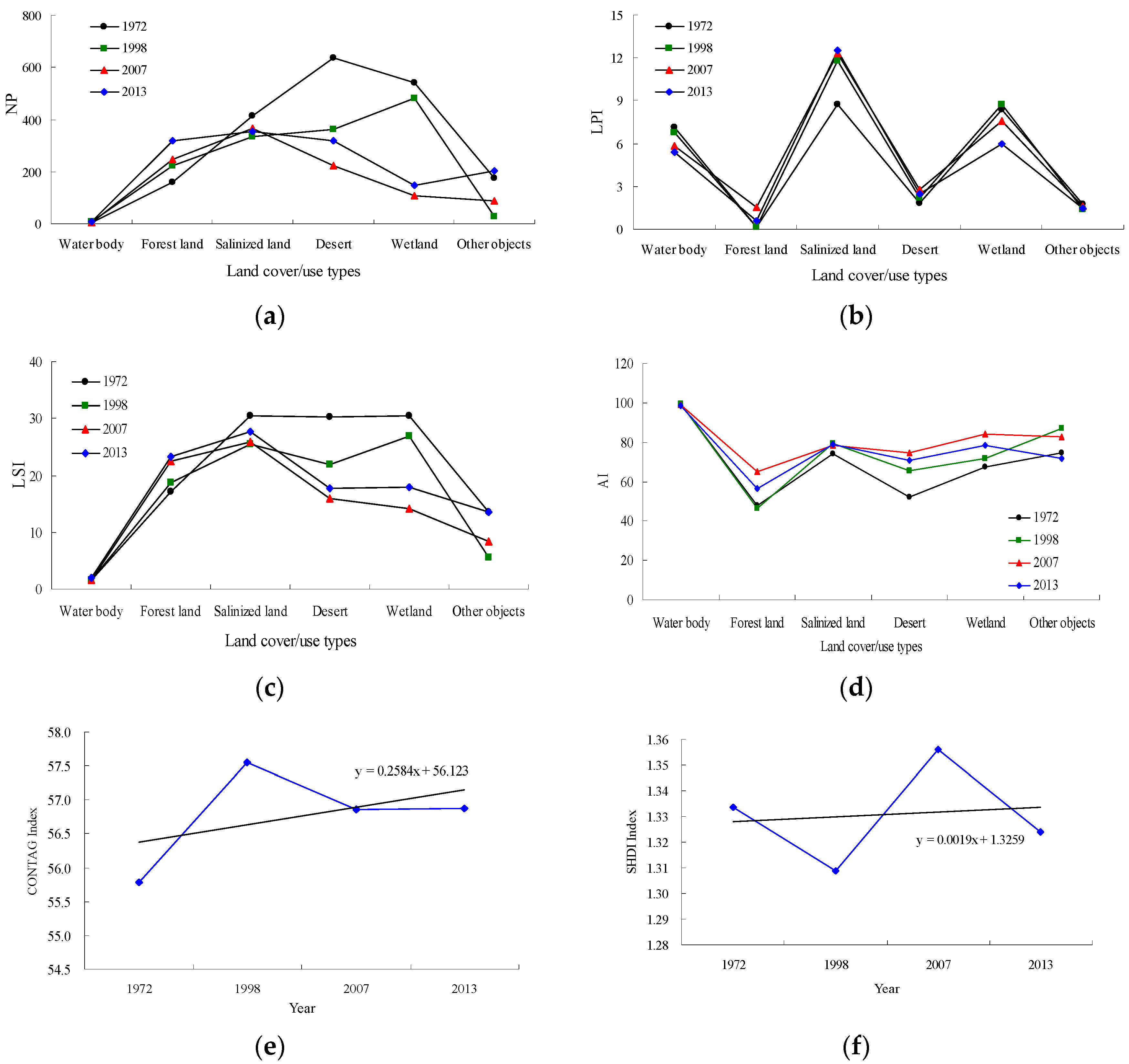
Comparison of (a) NP, number of patches; (b) LPI, largest patch index; (c) LSI, landscape shape index; (d) AI, aggregation index; (e) CONTAG, contagion index; (f) SHDI, Shannon diversity index; (g) SHEI, Shannon evenness index; (h) IJI, interspersion and juxtaposition index; and (i) FI, fragmentation index values, in the Ebinur Lake Wetland National Nature Reserve at five points in time: 1972, 1998, 2007 and 2013.
Figure 6.
Comparison of (a) NP, number of patches; (b) LPI, largest patch index; (c) LSI, landscape shape index; (d) AI, aggregation index; (e) CONTAG, contagion index; (f) SHDI, Shannon diversity index; (g) SHEI, Shannon evenness index; (h) IJI, interspersion and juxtaposition index; and (i) FI, fragmentation index values, in the Ebinur Lake Wetland National Nature Reserve at five points in time: 1972, 1998, 2007 and 2013.
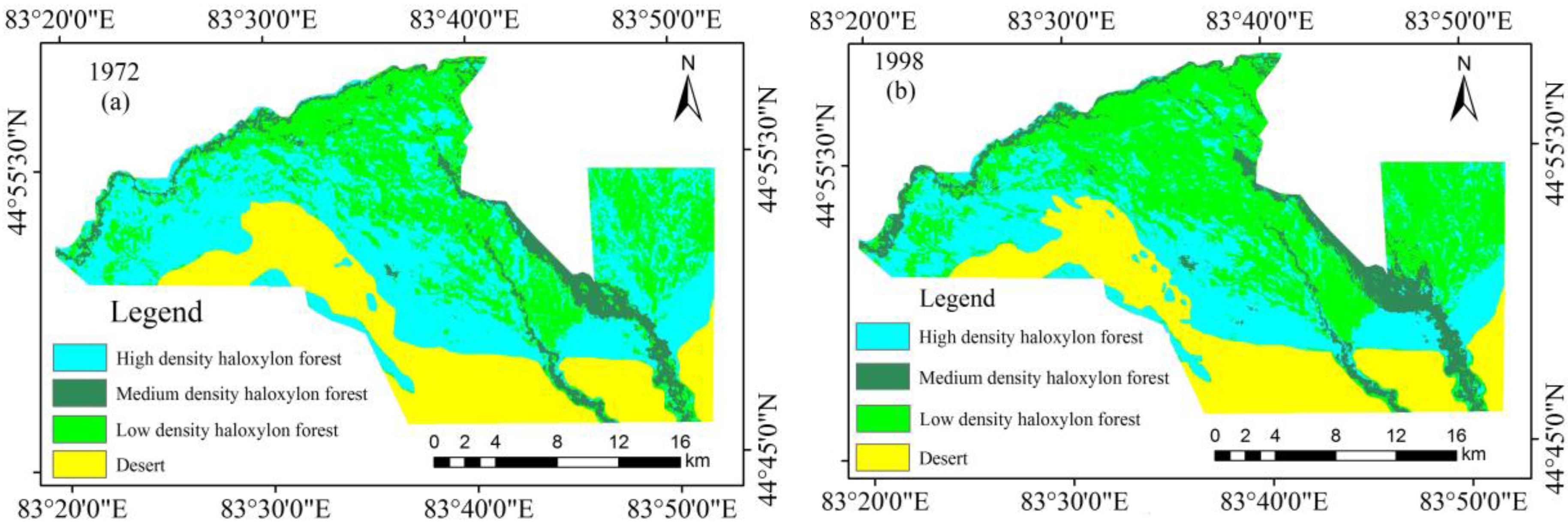
Figure 7.
Land-cover and land-use classification maps in Ganjia Lake Haloxylon Forest National Nature Reserve at five points in 1972 (a); 1998 (b); 2007 (c) and 2013 (d).
Figure 7.
Land-cover and land-use classification maps in Ganjia Lake Haloxylon Forest National Nature Reserve at five points in 1972 (a); 1998 (b); 2007 (c) and 2013 (d).
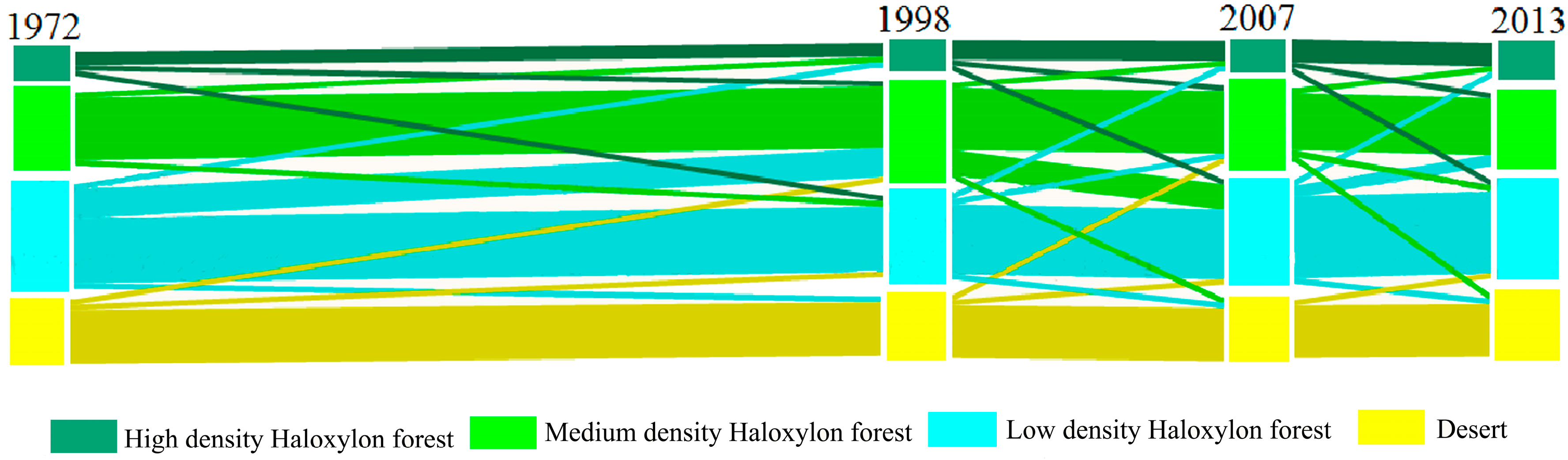
Figure 8.
Sankey diagram of land cover dynamics from the years 1972, 1998, 2007 and 2013 in the Ganjia Lake Haloxylon Forest National Nature Reserve.
Figure 8.
Sankey diagram of land cover dynamics from the years 1972, 1998, 2007 and 2013 in the Ganjia Lake Haloxylon Forest National Nature Reserve.
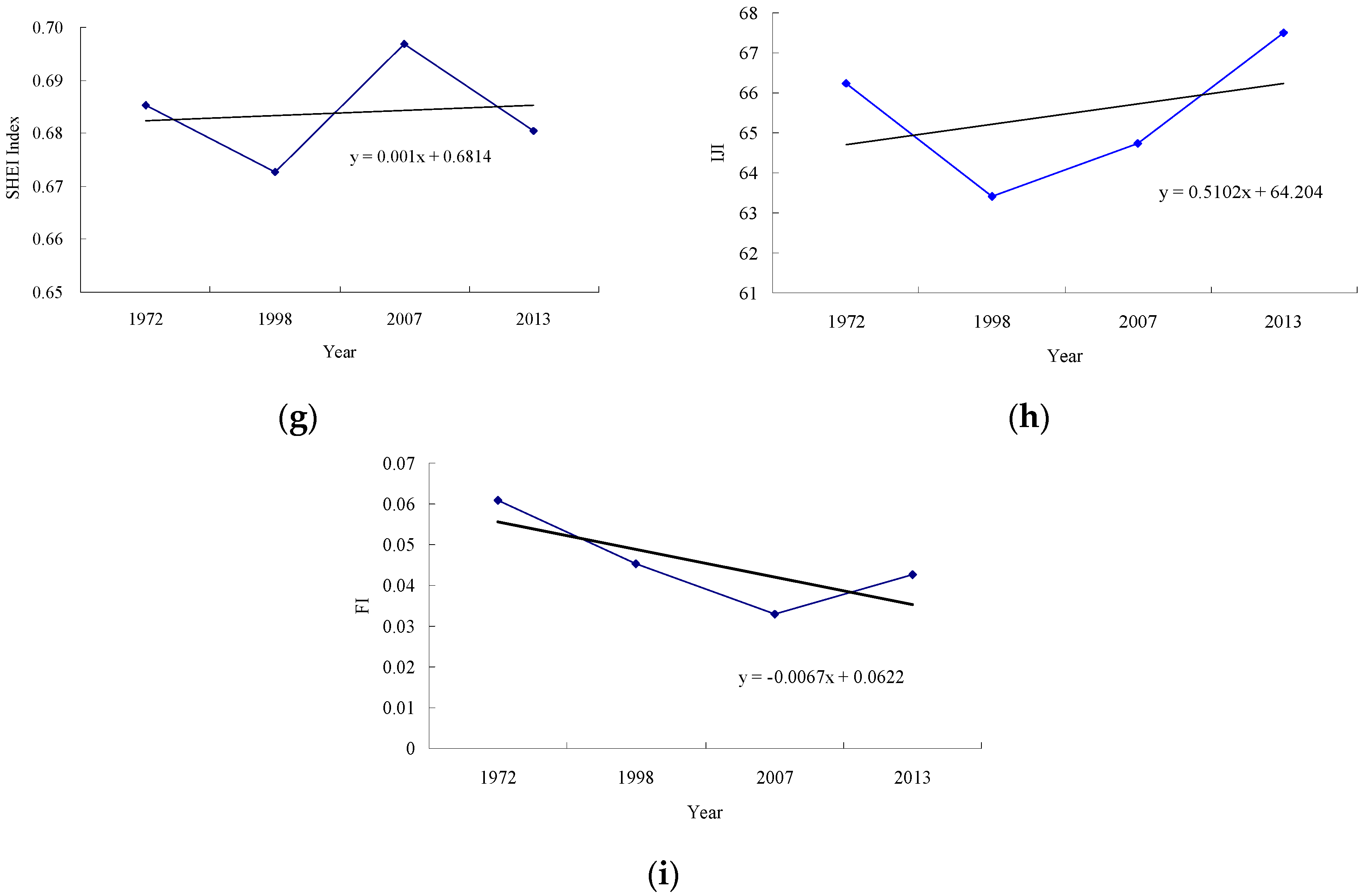
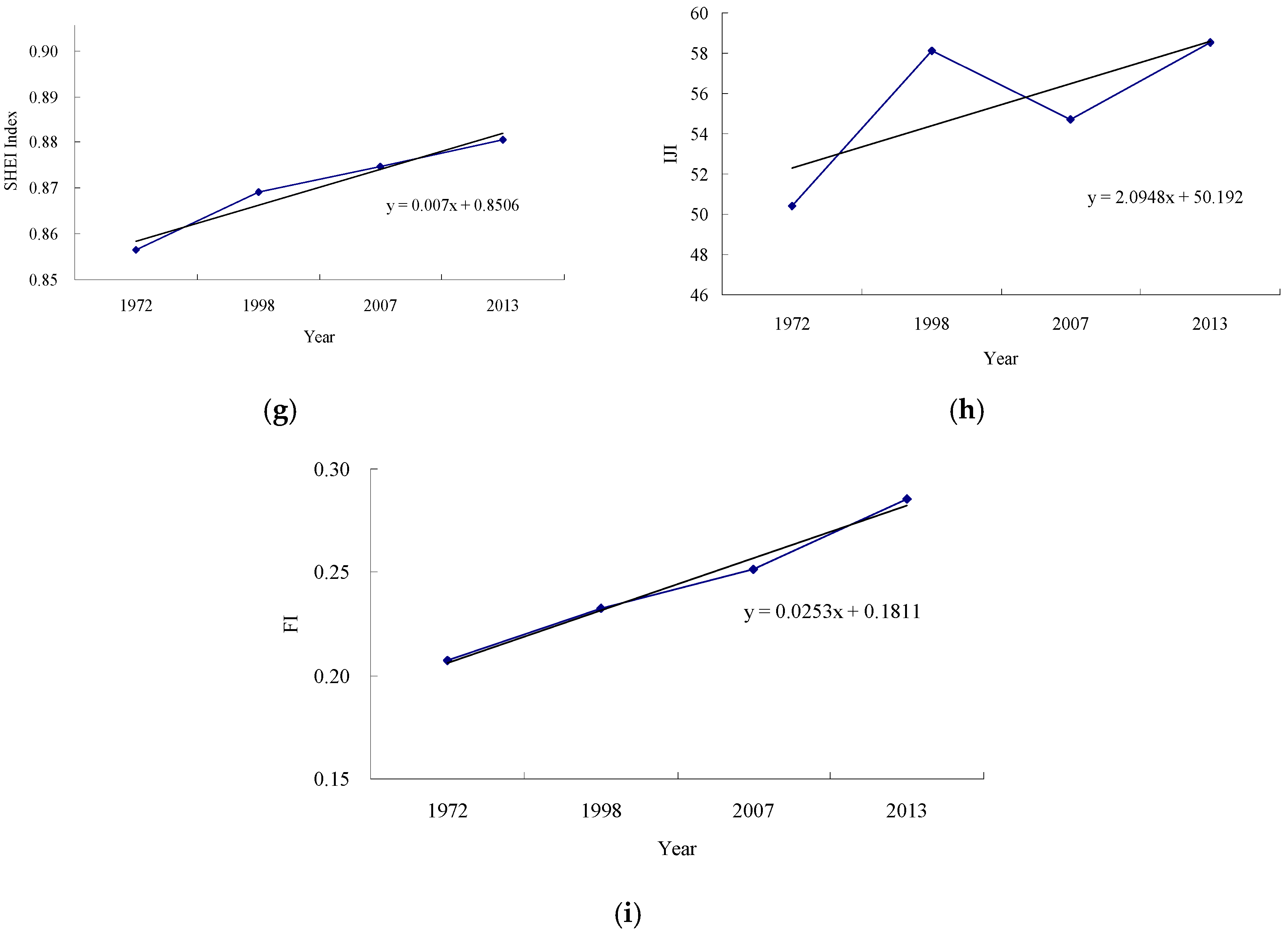
Figure 9.
Comparison of (a) NP, number of patches; (b) LPI, largest patch index; (c) LSI, landscape shape index; (d) AI, aggregation index; (e) CONTAG, contagion index; (f) SHDI, Shannon diversity index; (g) SHEI, Shannon evenness index; (h) IJI, interspersion and juxtaposition index, and (i) FI, fragmentation index, values in the Ganjia Lake Haloxylon Forest National Nature Reserve at five points in time: 1972 1998, 2007 and 2013. Note: LDHF, MDHF and HDHF are low, medium and high density Haloxylon forest, respectively.
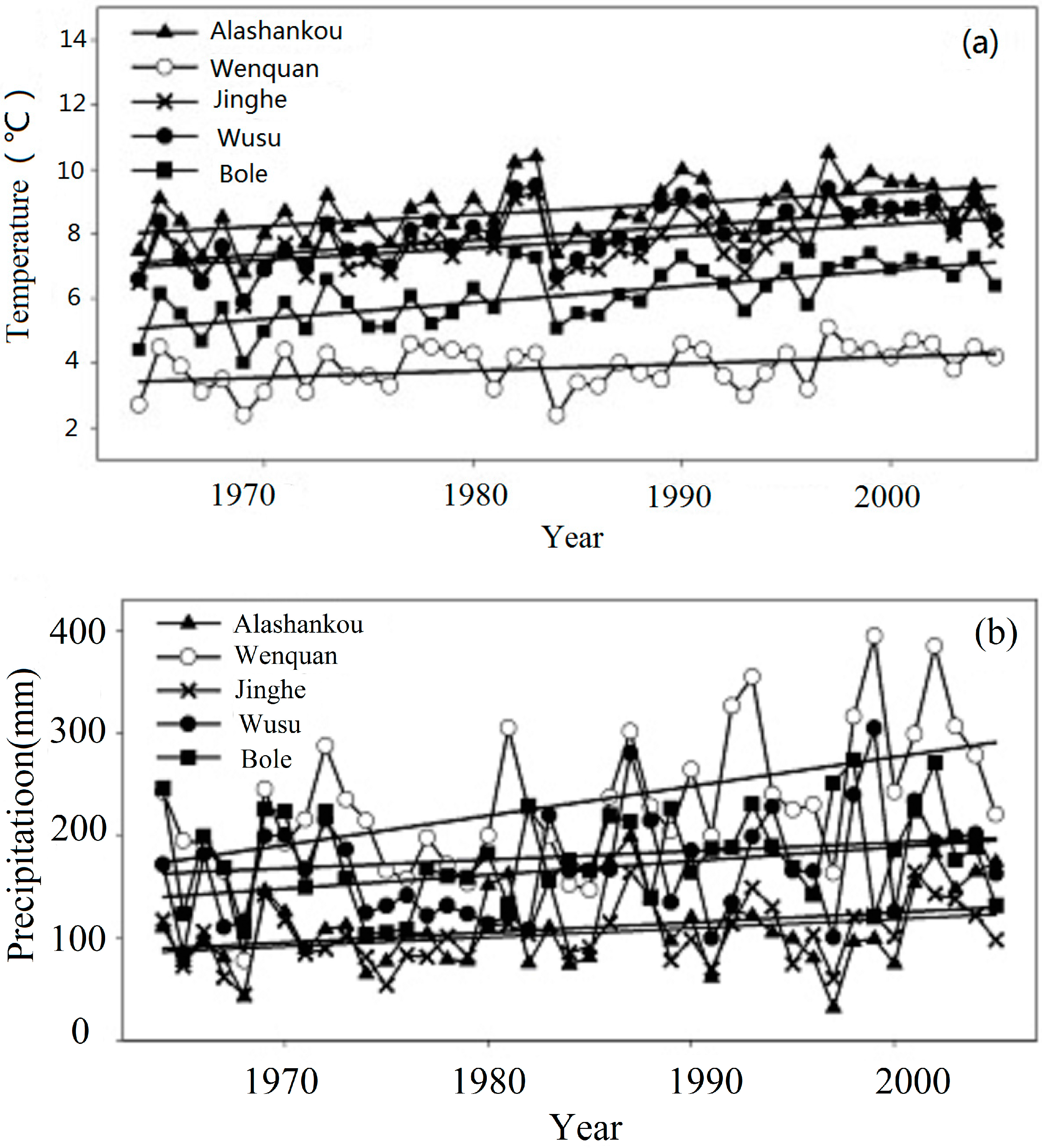
Figure 10.
Average annual temperature (a) and precipitation (b) for 1959–2005 at the Alashankou, Bole, Jinghe, Wenquan, and Wusu meteorological stations in the study area.
Figure 10.
Average annual temperature (a) and precipitation (b) for 1959–2005 at the Alashankou, Bole, Jinghe, Wenquan, and Wusu meteorological stations in the study area.
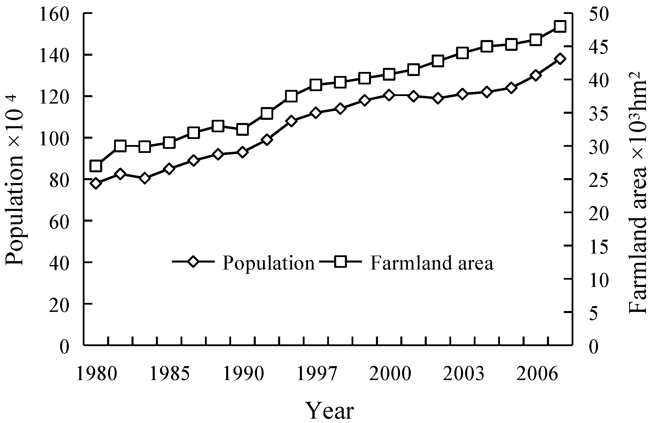
Figure 11.
The relationship between population and farmland are within the Ebinur Lake Watershed from 1980 to 2007.
Figure 11.
The relationship between population and farmland are within the Ebinur Lake Watershed from 1980 to 2007.
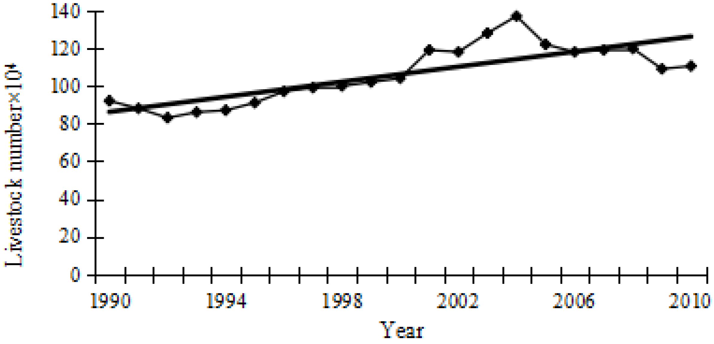
Figure 12.
The increased stocking levels for livestock in the Ebinur Lake Watershed from 1990 to 2010.
Figure 12.
The increased stocking levels for livestock in the Ebinur Lake Watershed from 1990 to 2010.
Table 1.
Data sources of landscape information in ELWNNR and GLHFNNR.
Table 1.
Data sources of landscape information in ELWNNR and GLHFNNR.
| Number | Imaging Data | Sensor | Resolution (m) | Spectral Bands |
|---|
| 1 | 21 September 1972 | MSS | 80 | B1, B2, B3, B4 |
| 2 | 25 September 1998 | TM | 30 | B1, B2, B3, B4, B5, B7 |
| 3 | 18 September 2007 | TM | 30 | B1, B2, B3, B4, B5, B7 |
| 4 | 26 August 2013 | OLI_TIRS | 30 | B1, B2, B3, B4, B5, B6, B7 |
Table 2.
Landscape metrics used in the present study.
Table 2.
Landscape metrics used in the present study.
| Index | Symbol | Definition | Formula |
|---|
| Number of Patches | NP | Number of patches divided by area. | NP = Ni |
| Largest Patch Index | LPI | LPI quantifies the percentage of total landscape area comprised by the largest patch. As such, it is a simple measure of dominance. | |
| Landscape Shape Index | LSI | A perimeter-to-area ratio that measures the overall geometric complexity of the landscape. LSI provides a standardize measure of total edge or edge density that adjusts for the size of the landscape. | |
| Contagion Index | CONTAG | Measures the extent to which patch types are aggregated or clumped. CONTAG is inversely related to edge density. | |
| Shannon’s Diversity Index | SHDI | SHDI is a popular measure of diversity in community ecology, applied here to landscape. SHDI is somewhat more sensitive to rare patch types than Simpson’s diversity index. | |
| Shannon‘s Evenness Index | SHEI | SHEI is expressed such that an even distribution of area among patch types results in maximum evenness. | |
| Interspersion and Juxtaposition Index | IJI | IJI is based on patch adjacencies, not cell adjacencies like the contagion index. | |
| Fragmentation Index | FI | FI is appealing because it reflects shape complexity across a range of spatial scales (patch sizes). | |
| Aggregation | AI | AI takes into account only the like adjacencies involving the focal class, not adjacencies with other patch types. | |
Table 3.
Changes in land use/cover types in the ELWNNR as measured in 1972, 1998, 2007 and 2013.
Table 3.
Changes in land use/cover types in the ELWNNR as measured in 1972, 1998, 2007 and 2013.
| Land Cover/Use Types | 1972 | 1998 | 2007 | 2013 |
|---|
| Area (km2) | Area Ratio (%) | Area (km2) | Area Ratio (%) | Area (km2) | Area Ratio (%) | Area (km2) | Area Ratio (%) |
|---|
| Water body | 538.44 | 16.98 | 506.66 | 15.98 | 437.56 | 13.80 | 406.77 | 12.83 |
| Salinized land | 1203.62 | 37.96 | 1243.42 | 39.21 | 1180.31 | 37.22 | 1371.44 | 43.25 |
| Forestland | 90.67 | 2.86 | 114.16 | 3.60 | 373.45 | 11.78 | 249.46 | 7.87 |
| Other objects | 229.76 | 7.25 | 128.52 | 4.05 | 171.73 | 5.42 | 200.74 | 6.33 |
| Desert | 354.47 | 11.18 | 380.53 | 12.00 | 351.22 | 11.08 | 354.06 | 11.17 |
| Wetland | 754.58 | 23.80 | 798.13 | 25.17 | 657.22 | 20.73 | 588.73 | 18.57 |
Table 4.
Calculation of confusion matrix by Maximum likelihood supervised classification in ELWNNR.
Table 4.
Calculation of confusion matrix by Maximum likelihood supervised classification in ELWNNR.
| | Water Body | Salinized Land | ForestLand | Desert | Wetland | Other Objects | Total | User’s Accuracy (%) |
|---|
| 1972 | Water body | 144 | 0 | 0 | 0 | 0 | 0 | 144 | 100 |
| Salinized land | 0 | 57 | 0 | 0 | 19 | 26 | 102 | 55.88 |
| Forestland | 0 | 46 | 101 | 0 | 0 | 0 | 147 | 68.71 |
| Desert | 4 | 0 | 0 | 114 | 0 | 0 | 118 | 96.61 |
| Wetland | 0 | 0 | | | 99 | 17 | 116 | 85.34 |
| Other objects | 0 | 0 | 0 | 0 | 0 | 77 | 77 | 100 |
| Total | 118 | 103 | 101 | 114 | 118 | 120 | Overall accuracy = 83.38% |
| Producer’s accuracy (%) | 99.61 | 55.34 | 100 | 100 | 91.67 | 64.17 | Kappa = 0.80 |
| 1998 | Water body | 99 | 0 | 0 | 0 | 0 | 0 | 99 | 100 |
| Salinized land | 0 | 121 | 0 | 0 | 7 | 0 | 128 | 94.53 |
| Forestland | 0 | 0 | 0 | 131 | 0 | 0 | 131 | 100 |
| Desert | 0 | 0 | 0 | 0 | 105 | 0 | 105 | 100 |
| Wetland | 17 | 0 | 71 | 0 | 0 | 0 | 88 | 80.68 |
| Other objects | 0 | 0 | 49 | 0 | 0 | 128 | 177 | 73.32 |
| Total | 116 | 121 | 120 | 131 | 112 | 128 | Overall accuracy = 89.97% |
| Producer’s accuracy (%) | 85.34 | 100 | 59.17 | 100 | 93.75 | 100 | Kappa = 0.88 |
| 2007 | Water body | 99 | 0 | 0 | 0 | 0 | 0 | 99 | 100 |
| Salinized land | 0 | 114 | 31 | 0 | 7 | 0 | 152 | 75 |
| Forestland | 17 | 0 | 0 | 120 | 0 | 0 | 137 | 87.59 |
| Desert | 0 | 0 | 0 | 0 | 104 | 1 | 105 | 99.05 |
| Wetland | 0 | 7 | 89 | 11 | 1 | 0 | 108 | 82.41 |
| Other objects | 0 | 0 | 0 | 0 | 0 | 127 | 127 | 100 |
| Total | 116 | 121 | 120 | 131 | 112 | 128 | Overall accuracy = 89.7% |
| Producer’s accuracy (%) | 85.34 | 94.21 | 74.17 | 91.6 | 92.86 | 99.22 | Kappa = 0.88 |
| 2013 | Water body | 111 | 0 | 0 | 0 | 0 | 0 | 111 | 100 |
| Salinized land | 0 | 76 | 0 | 0 | 15 | 21 | 112 | 67.86 |
| Forestland | 0 | 0 | 0 | 114 | 0 | 0 | 135 | 74.81 |
| Desert | 0 | 0 | 0 | 0 | 99 | 17 | 116 | 85.34 |
| Wetland | 7 | 27 | 101 | 0 | 0 | 0 | 135 | 74.81 |
| Other objects | 0 | 0 | 0 | 0 | 4 | 82 | 86 | 95.35 |
| Total | 118 | 103 | 101 | 114 | 118 | 120 | Overall accuracy = 86.5% |
| Producer’s accuracy (%) | 94.07 | 73.79 | 100 | 100 | 83.9 | 68.33 | Kappa = 0.84 |
Table 5.
Land-cover and land-use change transition matrix from 1972 to 1998, 1998 to 2007 and 2007–2013 (unit: % change).
Table 5.
Land-cover and land-use change transition matrix from 1972 to 1998, 1998 to 2007 and 2007–2013 (unit: % change).
| Periods | | Salinized Land | Wetland | Water Body | Desert | Forestland | Other Objects |
|---|
| 1972–1998 | Salinized land | 25.41 | 10.61 | 0.03 | 2.54 | 0.27 | 0.33 |
| Wetland | 7.93 | 12.17 | 0.77 | 1.81 | 0.24 | 2.28 |
| Water body | 0.00 | 0.05 | 15.92 | 0.00 | 0.00 | 0.00 |
| Desert | 3.64 | 0.63 | 0.00 | 6.44 | 0.58 | 0.70 |
| Forestland | 0.93 | 0.33 | 0.27 | 0.20 | 1.81 | 0.05 |
| Other objects | 0.00 | 0.01 | 0.00 | 0.16 | 0.01 | 3.87 |
| 1998–2007 | Salinized land | 27.03 | 9.02 | 0.13 | 0.88 | 0.15 | 0.00 |
| Wetland | 6.16 | 12.31 | 1.94 | 0.00 | 0.30 | 0.00 |
| Water body | 0.00 | 0.01 | 13.78 | 0.00 | 0.01 | 0.00 |
| Desert | 2.31 | 1.13 | 0.00 | 7.43 | 0.00 | 0.21 |
| Forestland | 3.62 | 1.87 | 0.13 | 3.04 | 3.12 | 0.00 |
| Other objects | 0.09 | 0.82 | 0.00 | 0.65 | 0.02 | 3.84 |
| 2007–2013 | Salinized land | 30.56 | 5.68 | 0.93 | 2.44 | 3.50 | 0.13 |
| Wetland | 3.87 | 14.40 | 0.16 | 0.00 | 0.13 | 0.01 |
| Water body | 0.01 | 0.09 | 12.72 | 0.00 | 0.01 | 0.00 |
| Desert | 1.05 | 0.00 | 0.00 | 8.17 | 1.24 | 0.71 |
| Forestland | 0.76 | 0.34 | 0.00 | 0.14 | 6.51 | 0.11 |
| Other objects | 0.96 | 0.21 | 0.00 | 0.31 | 0.40 | 4.45 |
Table 6.
Land-cover and land-use changes in the Ganjia Lake Haloxylon Forest National Nature Reserve as measured in 1972, 1998, 2007 and 2013.
Table 6.
Land-cover and land-use changes in the Ganjia Lake Haloxylon Forest National Nature Reserve as measured in 1972, 1998, 2007 and 2013.
| Land Cover Types | Area in 1972 (km2) | Area Ratio in 1972 (%) | Area in 1998 (km2) | Area Ratio in 1998 (%) | Area in 2007 (km2) | Area Ratio in 2007 (%) | Area in 2013 (km2) | Area Ratio in 2013 (%) |
|---|
| LDHF | 228.32 | 40.42 | 169.65 | 30.04 | 226.43 | 40.09 | 209.30 | 37.06 |
| MDHF | 166.52 | 29.48 | 215.32 | 38.12 | 150.68 | 26.68 | 163.15 | 28.89 |
| HDHF | 38.11 | 6.75 | 49.87 | 8.83 | 61.49 | 10.89 | 64.70 | 11.46 |
| Desert | 131.86 | 23.35 | 129.97 | 23.01 | 126.21 | 22.35 | 127.66 | 22.60 |
Table 7.
Calculation of confusion matrix by Maximum likelihood supervised classification in GLHFNNR.
Table 7.
Calculation of confusion matrix by Maximum likelihood supervised classification in GLHFNNR.
| | High Density Haloxylon Forest | Medium Density Haloxylon Forest | Low Density Haloxylon Forest | Desert | Total | User’s Accuracy (%) |
|---|
| 1972 | High density haloxylon forest | 33 | 3 | 0 | 0 | 36 | 91 |
| Medium density haloxylonn forest | 0 | 33 | 3 | 0 | 36 | 91 |
| Low density haloxylon forest | 0 | 8 | 84 | 0 | 92 | 91 |
| Desert | 0 | 0 | 0 | 94 | 94 | 100 |
| Total | 33 | 44 | 87 | 94 | Overall accuracy = 93.25 |
| Producer’s accuracy (%) | 100 | 75 | 96 | 100 | Kappa = 0.89 |
| 1998 | High density haloxylon forest | 43 | 3 | 0 | 0 | 46 | 93 |
| Medium density haloxylonn forest | 0 | 34 | 2 | 0 | 36 | 94 |
| Low density haloxylon forest | 0 | 6 | 86 | 0 | 92 | 93 |
| Desert | 0 | 0 | 0 | 94 | 94 | 100 |
| Total | 43 | 43 | 88 | 94 | Overall accuracy = 95 |
| Producer’s accuracy (%) | 100 | 79 | 97 | 100 | Kappa = 0.90 |
| >2007 | High density haloxylon forest | 36 | 3 | 0 | 0 | 39 | 92 |
| Medium density haloxylonn forest | 0 | 33 | 3 | 0 | 36 | 91 |
| Low density haloxylon forest | 0 | 8 | 84 | 0 | 92 | 100 |
| Desert | 0 | 0 | 0 | 94 | 94 | 100 |
| Total | 36 | 44 | 87 | 94 | Overall accuracy = 95.75 |
| >Producer’s accuracy (%) | >100 | >75 | >96 | >100 | >Kappa = 0.91 |
| 2013 | High density haloxylon forest | 39 | 3 | 0 | 0 | 42 | 92 |
| Medium density haloxylonn forest | 0 | 33 | 3 | 0 | 36 | 91 |
| Low density haloxylon forest | 0 | 12 | 80 | 0 | 92 | 86 |
| Desert | 0 | 0 | 0 | 94 | 94 | 100 |
| Total | 39 | 48 | 87 | 94 | Overall accuracy = 92.25 |
| Producer’s accuracy (%) | 100 | 68 | 91 | 100 | Kappa = 0.84 |
Table 8.
Land-cover and land-use transition matrix in the Ganjia Lake Haloxylon Forest National Nature Reserve from 1972 to 1998, 1998 to 2007 and 2007 to 2013 (unit: % change).
Table 8.
Land-cover and land-use transition matrix in the Ganjia Lake Haloxylon Forest National Nature Reserve from 1972 to 1998, 1998 to 2007 and 2007 to 2013 (unit: % change).
| Periods | | HDHF | MDHF | LDHF | Desert |
|---|
| 1972–1998 | HDHF | 5.61 | 1.85 | 1.60 | 0.01 |
| MDHF | 0.84 | 25.35 | 11.64 | 0.26 |
| LDHF | 0.24 | 2.05 | 26.67 | 1.01 |
| Desert | 0.00 | 0.16 | 0.65 | 22.06 |
| 1998–2007 | HDHF | 8.30 | 2.09 | 0.49 | 0.00 |
| MDHF | 0.27 | 25.43 | 0.67 | 0.31 |
| LDHF | 0.26 | 10.34 | 28.50 | 1.00 |
| Desert | 0.01 | 0.26 | 0.38 | 21.70 |
| 2007–2013 | HDHF | 9.61 | 0.60 | 1.24 | 0.00 |
| MDHF | 0.86 | 23.22 | 4.68 | 0.13 |
| LDHF | 0.39 | 2.58 | 33.51 | 0.58 |
| Desert | 0.02 | 0.28 | 0.66 | 21.64 |


