
Sustainable Governance of Organic Food Production When Market Forecast Is Imprecise

1
School of International and Public Affairs, Shanghai Jiao Tong University, Shanghai 200240, China
2
School of Business, Jiangnan University, Wuxi 214000, China
*
Authors to whom correspondence should be addressed.
Sustainability 2017, 9(6), 1020; https://doi.org/10.3390/su9061020
Submission received: 9 January 2017
/
Revised: 3 June 2017
/
Accepted: 5 June 2017
/
Published: 14 June 2017
(This article belongs to the Special Issue Sustainability in Food Supply Chain and Food Industry)
Abstract
:During the past few years, the market for organic food has been experiencing rapid growth. However, the market demand for organic food typically fluctuates due to its seasonal nature and customized characteristics, and it remains fairly difficult to precisely forecast market demand prior to the selling season. Forecast bias usually creates inefficiency in an organic food producer’s production plan and results in a substantial amount of waste. Thus, this paper studies how much an organic food producer is likely to lose with a certain level of forecast bias and investigates whether forecast bias necessarily results in an improper production plan. Finally, we calculate the maximum potential profit loss rate when the organic food producer determines how much to produce based on his forecasted demand, which we believe will be instructive for organic food producers in making production decisions. The target problem is formulated by a newsvendor model and solved using a tolerant analysis approach. We find that an organic food producer can still find the optimal solution only if his forecast bias is under a certain threshold. However, if the organic food producer’s forecast bias is beyond the threshold, he will probably make a sub-optimal production decision and potentially experience a profit loss. Subsequently, we analytically calculate an organic producer’s maximum potential profit loss rate for any given level of forecast bias. Examples are employed to numerically illustrate the main findings.
1. Introduction
Due in part to an increase in public awareness of environmental issues and interest in healthy foods, the proportion of organic food buyers among the general public has been rapidly increasing over the past few years. The global organic food market is projected to register a compound annual growth rate (CAGR) of over 16% from 2015 to 2020 and to reach USD211.44 billion by 2020 [1]. The basic and critical question in the food industry is the link between intensive mass production and market demand [2]. Regarding market demand, evidence suggests that the market demand for organic food continuously fluctuates due to several factors, such as environmental challenges, high purchase prices, organic food availability, income levels, government initiatives and consumer familiarity and awareness [3]. In addition, periodical organic crop plantation, processing complexity and long-distance shipment make the supply of organic foods time-consuming. To determine how much to supply, organic food (OF) producers must perform market forecasts at the time of planting. However, it is a challenge to achieve a precise market forecast at a time long before the selling season [4]. For example, it takes farmers approximately 2–4 months to grow organic corn from sowing to harvest in addition to preparation time, depending on the types of corn that are planted and the climate it is grown in. A world leading market consulting company predicted the global market volume of organic food in 2015 would be about 99.45 billion U.S. dollars [5]. Because of the uncertain factors in market, the global market sales of organic food was only 81.6 billion U.S. dollars, nearly 20% less than the prediction, in that year [6]. Therefore, the difficult task of creating a market forecast for organic food can be characterized by a long period of harvest time, fluctuating demand, rapidly changing consumer awareness and market circumstances [7,8]. Thus, various approaches are employed to forecast demand. For example, household surveys [9], multi-variable regressions [10], data mining [11], group discussions [12] and case studies [13] have been adopted to forecast the demand for food. Generally, the precision of a food demand forecast varies from case to case [14], which directly affects the profit of the decision makers.
To enrich the soil in which organic food grows, numerous techniques are used as alternatives to toxic and persistent pesticides, herbicides and synthetic nitrogen fertilizers. These techniques include hand weeding, mechanical control, cover crops, crop rotation and dense planting [15]. Therefore, organic food normally costs 20–100% more than conventional food, and a failure to accurately forecast demand can result in a large potential loss due to the waste of resources or selling opportunities [16,17]. Statistical- and simulation-based research has been performed by Lse [18] and Weatherford and Belobaba [19], respectively. They assert that the negative impacts of demand forecasting inaccuracy increase proportionately with the percentage error in airline revenue management. Therefore, a number of papers have analyzed how an imprecise demand forecast influences the decision maker’s expected profit. Previous related research has focused on disclosing the underlying reasons for food (and organic food) wasting on the way from farm to the end consumer [14,20,21], as well as several tools to measure the waste in the whole life cycle of food product (summarized by Strotmann [22]) and some solving mechanism by operational activities in supply chain [23,24,25,26]. These papers try to reduce food waste and improve the performance of one decision maker or the entire supply chain at different decision situations. Similar to the existing studies, we focus on reducing the waste of resources and selling opportunities in organic food production at a different situation that the demand forecast is not precise.
As previously stated, a demand forecast is made during the production preparation period, whereas the actual demand is known at the beginning of the selling season. The difference between forecasted demand and actual demand is termed forecast bias. Forecast bias often occurs and typically means inefficient production and waste of resources or selling opportunities [27]. Vollmann et al. [28] shows that forecast bias directly affects decisions on customer service and the reserve stock level. Therefore, we provide an approach to the quantitative analysis of the potential profit loss in organic production when demand forecast is not precise, which we believe would be helpful to OF producers in formulating a production plan and further enhance its governmental sustainability in food production. In recent years, the term “sustainable governance” becomes very familiar and is well-documented in the literature. Sustainable governance aims to provide effective governance of resources for long-term development by new forms of collective decision-making at local level [29,30,31]. In this paper, we try to enhance sustainable governance of organic food production by suggesting an optimized decision-making approach. The specific questions that we seek to answer in this study are as follows:
- Since forecast bias occurs often, how much of the OF producer’s profit is negatively affected?
- Because improving forecast precision is costly, a certain level of forecast bias is likely to be acceptable to OF producers. Is there a forecast bias threshold under which the OF producer can still make optimal (or near-optimal) decisions?
- It is common and reasonable for an OF producer to evaluate the risk of a decision regarding production quantity. Is it possible to analytically evaluate the OF producer’s maximum potential profit loss when he formulates production plans according to an imprecise demand forecast?
After being introduced in Morse and coworkers’ book [32], newsvendor model has been widely employed in operational management and applied economics [33]. In this study, the OF producer aims to determine his optimal production quantity by balancing the expected cost and revenue with uncertain demand information. Because the OF producer’s decision falls into the structure of a newsvendor problem, we formulate the OF producer’s problem by a newsvendor model. The producer’s maximum expected profit is achieved by optimizing the product output quantity of the proposed newsvendor model. Based on sensitivity analysis of the optimal product output quantity achieved by the newsvendor model, the specific questions mentioned above are answered.
Actually, several existing studies focus on organic food production and suggest principles or experiences, according to which a sustainable decision can be made [34]. However, few researchers have analytically studied the production decision under the unreliable demand forecast. At the same time, a number of technical-related studies in the operational management field focus on production/capacity decisions with unreliable forecast/demand using newsvendor models. For example, Scarf [35] studied an inventory problem in which only the standard derivation and the mean of demand were forecasted. Because the solution is not affected by the distribution of demand, the method Scarf [35] proposed is often referred to as the “Scarf rule”, which is extended to problems with more general settings. For example, Yue et al. [36], Perakis and Roels [37] and Zhu et al. [38] propose a new robust model that minimizes the maximum profit loss of decision makers using only the known mean and standard derivation of demand. However, the mean and standard derivation are typically not precisely known in practice [39]. More often, a set of historical observations and future trends rather than the exact mean and standard derivation are available. Indeed, it is reported that many small companies rely on the historical data to forecast future demand [40]. Thus, we contend that the previously described theoretic findings considering known mean and standard derivation of demand are less applicable in many practical situations. Therefore, Wang et al. [39] assume a product output problem in which the demand distribution is forecasted but the shape parameters are unknown. These researchers adopt historical observed demand data to find the boundaries of the shape parameters by using the data achieve a certain level of likelihood. The proposed model is solved using a robust optimization approach. However, robust optimization often suggests pessimistic solutions given the limited demand information (i.e., only the known mean and standard derivation, the distribution type and historical data). Generally, a newsvendor makes his decisions only using his forecasted demand (based on, e.g., historical data or market-trend analysis) rather than the exact value of the mean and derivation or a specific distribution type of the demand. Differently from the cited studies, we do not provide pre-determined shape parameters of market demand (e.g., mean value, distribution or standard derivation) and study the OF producer’s optimal solutions with a known forecast bias. In sum, the primary contribution of this study has two aspects. (1) The effects of forecast bias on the OF producer’s expected profit and optimal solution are analytically studied. Whereas similar research empirically or statistically studies the influence of forecast bias on the decision-making process, we study the problem using a method based on strict mathematical deductions; (2) Although the proposed newsvendor model with non-linear constraints is prohibitively difficult to solve, we analyze the model using a tolerance-analysis approach and finally arrive at several close-form solutions.
The remainder of this paper is summarized as follows. In Section 2, we provide a literature review. Section 3 presents a benchmark model and describes the construction of the OF producer’s decision model. Next, we analyze the relations between forecast bias and optimal solutions. In Section 4, we calculate the OF producer’s maximum potential expected profit loss with forecast bias. Section 5 summarizes and concludes the paper.
2. OF Producer’s Sustainable Production Decision Model
Organic food is prepared and processed without using chemical fertilizers, pesticides or preservatives and has been popular in recent years. Similar to conventional food production, organic food production starts from land consolidation and ends at the packaging of final products. Many time-consuming processes are involved, including resource preparation, seed sowing, pest control, harvest and processing. For example, the soil has a profound impact on the quality of the final product and must be aerated as in the natural world with farm-derived organic matter and mineral particles. Generally, the OF producer requires approximately one month to prepare the soil for planting. Subsequently, the seeds require several months to mature until harvest and several additional weeks or months for processing into market-ready organic food. Since organic food production is time-consuming, the OF producer must formulate his production plan based on a demand forecast created long before the product is sold. The OF producer’s decision process can be divided into two stages. During the first stage, the producer determines the production quantity based on the demand forecast and conducts preparation and production. During the second stage, the actual demand distribution is known based on updated market information, and the OF producer allocates products to consumers. The OF producer’s activities are presented in Figure 1.
OF producers aim to maximize expected profit with a certain amount of product output, which can be formulated using a classic newsvendor model that considers selling price, production cost and salvage value. Forecasted market demand follows a discrete distribution, with probability mass function and cumulative distribution function . When the output product quantity is , the OF producer’s expected profit under forecasted demand is denoted by . The OF producer’s expected profit function consists of two parts, the revenue from selling products and the salvage of over-produced products, the expense in production. Obviously, the OF producer’s objective is to maximize his expected profit by determining the optimal production quantity. Since the newsvendor model is a mathematical model used to determine optimal decisions by balancing the expected cost and revenue with some uncertain factors [41], the OF producer’s production problem can be formulated by a newsvendor model (Equation (1)).
In Equation (1), , is the profit when demand is , and the output quantity is , , and denote the selling price, purchasing cost and salvage value, respectively. The optimal production quantity of the OF producer can be determined by solving Equation (1). In fact, several operational studies [42,43] suggest an optimal solution, which can help decision makers determine production quantity due to uncertain demand. The solution is provided by Equation (2).
In Equation (2), is normally called the critical fractal [44], which is denoted by for mathematical convenience in this paper. In practice, the selling price, salvage value and production cost of organic food are exogenous and known to OF producers. Similar to other products in different industries, the market demand for organic food is easily affected by many factors, such as consumer income, preferences and the price of substitute products. Additionally, because organic food production starts as early as the plantation of organic crops, it is difficult to conduct a market forecast. Therefore, the market demand for organic food typically fluctuates and is often estimated using historical data and experience. As discussed by many researchers and industry experts, occasionally, there is a large difference between the forecasted demand and actual demand [45], which results in some well-documented business failures. This is why Cisco, a major networking equipment supplier, had to write off 201 billion U.S. dollars in excess stock in 2001 [46]. The difference, which we term forecast bias in this paper, typically affects the OF producer’s production decisions and expected profit. According to industrial statistical data, a producer is expected to suffer 0.48 to 1.78% profit loss if the market demand is over-forecasted by 25% [19]. Because the demand forecast for organic food is made as early as the soil preparation stage when less market information is available, a forecast bias often occurs in practice. Therefore, decisions on output quantity based on forecasted demand are likely non-optimal. In the following section, we analyze the degree to which an OF producer’s decisions are biased because of market forecast bias.
3. OF Producer’s Production Decision with Imprecise Demand Forecast
Because of uncertain factors in markets, demand is usually deemed as a random variable in academia and industry [47]. Historical and empirical data indicate that market demand for organic food is random and ranges in an underlying sample space, whose upper and lower bounds are the demands at the most positive and pessimistic situations, respectively [48]. Meanwhile, demand for organic food in a region is normally counted in billions (e.g., [49,50,51,52,53]) or millions (e.g., [54,55,56,57,58]). Thus, the set of all possible outcomes of random demand in a sample space is estimable and countable. Similar to many existing studies (e.g., [59,60,61]), we assume the demand for organic food as a random variable following discrete distributions.
The probability vector of the forecasted demand for organic food can be denoted by . Since demand forecast might not be precise, the actual demand probability vector is specified by , where is a perturbation vector . Since demand probability vectors are non-negative, are non-negative. Obviously, if the perturbation vectors equal zero, the forecasted demand is precise, and the OF producer can determine the optimal production quantity based on the forecasted demand. Because the actual demand probability vectors can be quite different from those in forecast, the distributions and its shape values of the forecasted demand and the actual demand may differ. Figure 2 shows that, when forecasted demand and forecast bias is known, the ranges in which actual demand possibly locates in are thereby estimated and depicted as the shaded area. In this paper, we do not focus on what distributions or what the shape values of the forecasted demand and actual demand are, we are most interested in the influence of forecast bias, i.e., , to the OF producers’ production decisions and expected profits.
Because the sum of all demand probabilities equals 1 and each of the probability factors is in the range [0, 1], valid perturbations follow and . Obviously, we could arrive at the OF producer’s optimal production decision when the perturbation vectors are known. However, a producer’s demand probability vector is estimated by forecast and is likely inconsistent with the real probability vector, whereas the forecast bias is easily evaluated by producers [62]. On this basis, we assume all perturbation vectors vary in a certain range for an OF producer and let be the OF producer’s forecast bias, such that . Obviously, the probability factors after any perturbation are still non-negative.
Remark 1.
The demand probability vectors of forecasted demand might differ from that of the actual demand, and the difference might be negative or positive values. For example, the estimated demand for a product in Theodore’s gift shop is one value from demand sample space {5, 6, 7, 8} with probability vector {0.2, 0.25, 0.3, 0.25} [63]. Especially, the probability that the value of demand equals 5, 6, 7 and 8 are 20%, 25%, 30% and 25%, respectively. If the actual demand probability vector differs, the probability vectors become to be . When for all , we find the sum of all demand probability vectors . Meanwhile, the sum of all demand probability vectors is less than 1 when for all . Since the sum of all demand probabilities certainly equals 1, not all are bigger than 1 or smaller than 1. Therefore, when one (several) perturbation vectors is (are) smaller than 1, there exists at least one perturbation vector that is bigger than 1. The finding indicates that the difference between probability vectors of actual demand and that of forecasted demand simultaneously includes non-positive and non-negative values. Based on the above analysis, we assume the demand forecast bias to be a bi-directional.
We are most interested in one important question: What is the optimal production quantity under a given biased forecast? We analytically answer the question by Proposition 1 and Corollary 1.
Proposition 1.
if and only if
Proof.
See Appendix A.
As defined in Section 2, denotes the term and is the cumulative distribution function of the random demand. Proposition 1 provides the value of when potentially is the optimal solution of the production problem with an unreliable demand forecast. Because many demand forecasting/evaluating technologies are proposed in the literature, such as the causal method, time-series analysis and the expert systems method [64], different forecasting technologies have different limitations and evaluation preciseness. However, the potential optimal solutions regarding the actual demand are estimated by Proposition 1. That is, if the OF producer’s forecast bias is known, we can determine whether the production quantity based on demand forecast is still the optimal production decision.
However, it remains unclear whether the optimal decision with a precise forecast still holds when the demand forecast bias is small. How much demand forecast bias is permitted such that the decision made based on the forecasted demand remains identical with that based on actual demand? Based on Proposition 1, we have the tolerance of demand forecast bias that leads to (see Corollary 1).
Corollary 1.
We have if and only if
Proof.
See Appendix A.
Corollary 1 suggests the maximum tolerance of the forecast bias that the OF producer’s decision based on an imprecise demand forecast is the same as that based on actual demand. It is intuitionally known that the demand forecast bias negatively links to the OF producer’s benefit. However, Corollary 1 highlights that OF producers’ production decision is still optimal with an imprecise demand forecast only if the forecast bias is within a certain range. Different from the traditional belief that demand forecast bias results in biased decisions and harms the decision maker’s expected profit, Proposition 1 and Corollary 1 suggest that a certain level of demand forecast bias does not influence the OF producer’s quantity decision. Therefore, the OF producer’s decision based on a biased demand forecast is the same as that based on actual demand. We believe that this conclusion represents an instructive contribution to the organic food industry in determining how much to produce. Since the mathematical expressions of Proposition 1 and Corollary 1 are not easily understood by general readers, we employ Numerical Study 1 to represent the implications of those expressions.
Numerical Study 1.
We consider an OF producer’s production problem as follows: the selling price is $10, the salvage value is $2, and the production cost is $8. The forecasted demand is presented in Table 1. For example, the possibility vector that demand equals 200 units in the OF producer’s forecast is 10%.
We can employ Proposition 1 to calculate the minimum level of demand forecast bias that the production quantity by forecasted demand is the optimal solution. For example, when we introduce 201 units as the demand vector into Proposition 1, we can conclude that is a value larger than 0.2727. This result indicates that the optimal production quantity for the actual demand distribution is 201 units only if the demand forecast bias level is larger than 0.2727. That is, if the demand forecast bias level is smaller than 0.2727, the optimal production for the actual demand distribution is definitely not equal to 201 units. Similarly, the minimum demand forecast bias level for each value in Table 1 can be calculated using Proposition 1 (Table 2).
Table 2 is highly useful to the OF producer in determining optimal production quantities. For example, when the OF producer’s demand forecast is unreliable and the level of forecast bias is 1, the OF producer is advised by Table 1 that the optimal production quantity for the actual demand distribution is definitely one value in 201 units, 202 units and 203 units. We term the candidate values, i.e., 201, 202, 203, “candidate solutions” (Table 2). Therefore, the OF producer’s optimal decision regarding production quantity with the unknown actual demand information should be one of the three values. Similarly, the OF producer’s optimal production quantity is a number in 202 units and 203 units when the level of demand bias is less than 0.2. Although the OF producer’s actual demand distribution is unknown, the optimal production decision is expressed in finite candidate values calculated by Proposition 1.
In particular, when the OF producer’s level of demand forecast bias is less than 0.087, the only candidate value of optimal production quantity is 202 units (Table 2). Because of , we have when is less than 0.087. Therefore, we are able to further calculate the variation of probability vector for . For example, if the probability of is 0.25 in forecast (Table 1 and Figure 3), i.e., , we have the range of probability vector after perturbation , i.e., (Figure 3). Thus, when forecast bias is less than 0.087, the real probability sector of ranges (0.092, 0.1). Similarly, we have the ranges of probability towards other demand vectors (Table 3).
Since the production decision by imprecise demand forecast is still optimal as long as forecast bias is less than 0.087, Table 3 suggests the corresponding ranges of real probability sectors. We visually represent the values in Table 3 by Figure 3, where the shaded areas denote the ranges of real probability vector. This result suggests that the OF producer’s production decision based on the forecasted demand with a certain forecast bias can be the same as that based on the actual demand (Figure 3). Thus, the finding presented by Corollary 1 is very useful.
According to a report by Fox News [65], organic food typically cost 20–100% more than their conventional counterparts. Thus, many consulting or educating organizations, including 10 great colleges in the U.S., are thereby built to provide services to reduce the cost of growing organic food [66]. The finding represented by both Corollary 1 and Figure 3 suggests another way to enhance the profitability of the organic producer. Rather than reducing the cost of growing organic food, improving forecast imprecision to a certain level can reduce the waste and increase profit in return.
4. An Approach to Evaluating the OF Producer’s Maximum Profit Loss
The OF producer is more likely to make a biased decision regarding production when his demand forecast bias is large. It is instructive for the OF producer to identify how much he can potentially lose when he makes production decisions based on the forecasted demand. On the one hand, the OF producer potentially loses because a forecast is imprecise. On the other hand, forecast precision can be improved through investment. For example, if the cost invested in forecast improvement is less than the reduced potential loss, the OF producer is motived to improve his forecast precision. Thus, in this section, we primarily study the relations between the level of demand forecast bias and the expected profit loss when the OF producer makes production decisions using his forecasted demand.
The performances of the evaluated values are typically modeled as the expected profit differences compared with ideal situations (e.g., [67]). To inflect the influence of demand forecast bias, we specify the profit loss using a fractal structural model, which we formally represent by Definition 1.
Definition 1.
For a value of the OF producer’s forecast-bias level , we let , where . We state that is the maximum profit loss rate under forecast-bias .
Definition 1 formally suggests the formulation of the OF producer’s maximum profit loss rate when he makes production decision under forecast-bias . As described by Proposition 1, we have the solution space for any given forecast bias . Therefore, can be transformed as follows:
Because indicates that the optimal solution of the OF producer is , i.e., (Equation (2)). Thus, is the expected profit, and is the optimal production quantity with actual demand. Since is the expected profit producing with the forecasted demand, consisting of and denotes the expected profit loss rate of producing with the demand forecast when is the optimal production quantity. For a given value of forecast bias , it is straightforward to calculate the value of by solving Equation (3). However, it is burdensome to solve the difficult NP-hard problem of the nonlinear programming of Equation (3). Therefore, we find that it is possible to reduce the calculation burden by Proposition 2.
Proposition 2.
For any given , .
Proof.
See the Appendix A.
From Proposition 2, we find that the maximum profit loss rate only occurs at two-tailed values of candidate solutions. Comparing the profit loss rate at the tailed values saves substantial calculation time when there are many candidate solutions. For example, when the demand for organic food consists of many discrete values or the forecast bias is large, more vectors are included in the candidate solutions. In such cases, we save substantial calculation time by calculating only two-tailed values in the candidate solutions.
In addition, we employ Corollary 2 to represent the maximum profit loss rate when . This finding indicates that the investor can also pre-judge the maximum potential profit loss rate when the demand forecast bias is completely unknown.
Corollary 2.
When , we have
Proof.
Refer to Appendix A.
The findings for Proposition 2 and Corollary 2 represent a simple means to compute the value of the OF producer’s maximum expected profit loss rate. Numerical Study 2 is used to illustrate how our findings are applied in practice and to visually present the OF producer’s maximum expected profit loss rate under different levels of demand forecast bias.
Numerical Study 2.
We employ the same OF producer’s problem used in Numerical Study 1 and find the OF producer’s candidate solutions for each level of demand forecast bias based on the values in Table 2. Thus, we present the OF producer’s candidate solutions in Table 3.
As shown in Table 4, the number of candidate solutions increases according to the level of forecast bias. For example, when the level of forecast bias is in the range [0, 0.087), the only candidate solution is 202 units. In this case, the OF producer’s optimal production quantity is 202 units.
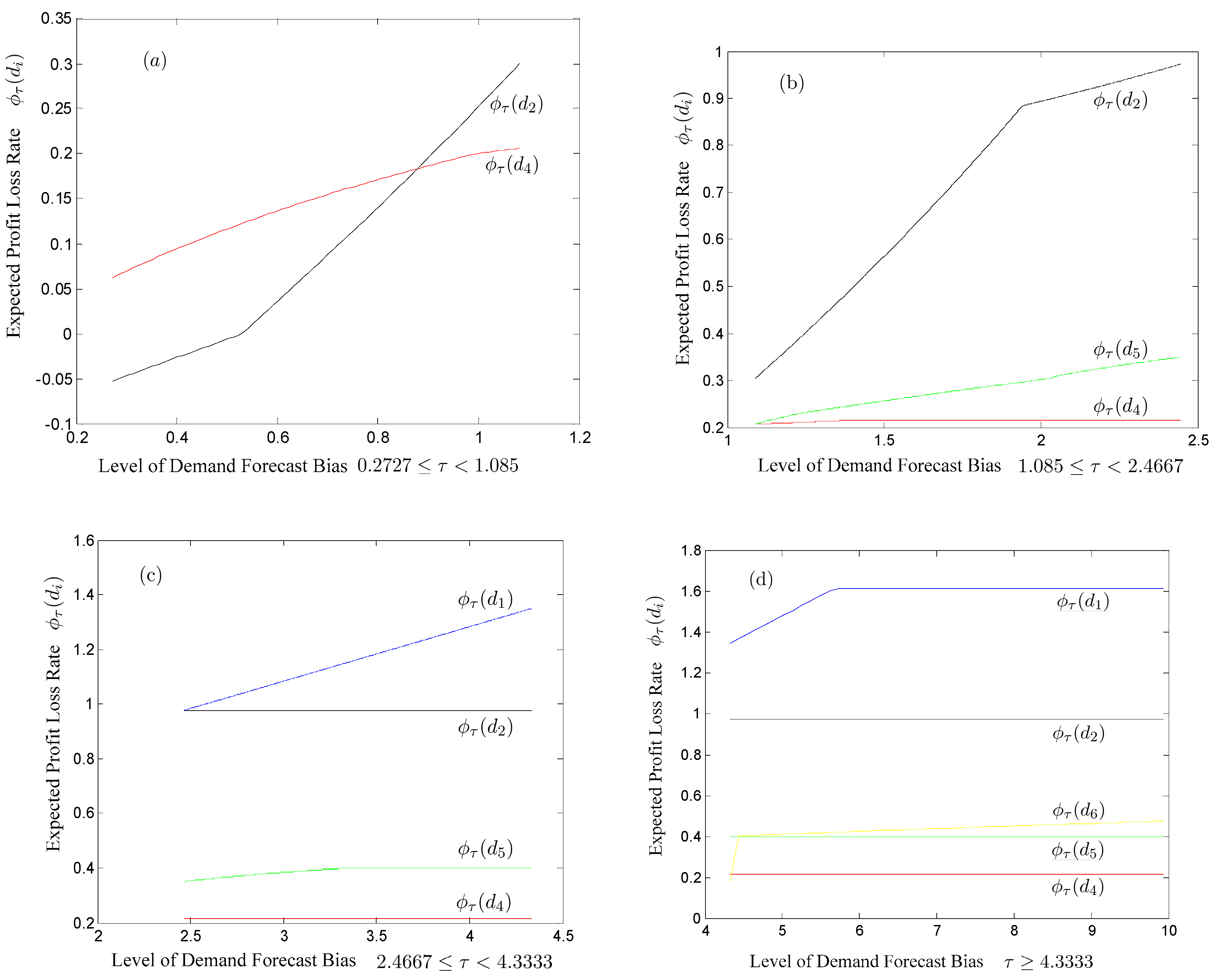
In Figure 4 and Figure 5, we present the expected profit loss rates in candidate solutions when we make productions with imprecise demand forecast. For example, when forecast bias is in range [0.2727, 1.085), the profit loss rates respecting to two candidate solutions, i.e., 201 units and 202 units, are as in Figure 5a. Expected profit loss rates when forecast bias ranges in other intervals are presented in Figure 5b–d. We also observe that the maximum value of expected profit loss rate for a given level of forecast bias occurs on the tailed values of the solution space, which highlights the theoretical finding in Proposition 2.
We believe that the expected profit loss rates in Figure 4 and Figure 5 help the OF producer identify the expected profit loss rate before he determines his production quantity based on the forecasted demand. For example, when forecast bias is 2, we have . According to Equation (3), the maximum profit loss rate when forecast bias is , i.e., for . Similarly, the maximum profit loss rate with respect to each value of forecast bias is calculable and their relations are represented in Figure 6.
Figure 6 suggests the OF producer’s maximum potential profit loss rate with different levels of forecast bias. It is observed that the OF producer’s maximum potential profit loss rate non-decreases by the forecast bias. However, when the demand forecast bias is less than 0.0667, the OF producer’s production quantity is the same as when the actual demand distribution is known to the OF producer. This observation highlights our finding in Corollary 1, which we believe is instructive for OF producers. Although maximum potential profit loss rate non-decreases by the forecast bias, we find from Corollary 2 that the maximum potential profit loss rate levels off to a certain value. For example, the numerical study described in Figure 6 suggests that the OF producer’s maximum profit loss rate levels off to 1.61. Because the OF producer’s expected profit with actual demand is a non-negative value, the profit loss rate, which is larger than 1, indicates the OF producer’s expected profit with his forecasted demand is a negative value. In this example, when forecast bias is larger than 2.4667, the OF producer’s expected profit with the forecasted demand is likely to be a negative value, which means that the producer possibly confronts a loss due to imprecise demand forecast. Thus, the proposed risk-evaluating of Proposition 2 is helpful to OF producers to evaluate the risk of failure before making their production plans. This observation presented in Figure 6 also indicates the importance of providing precise demand forecast in organic food industry and explains why so many third-party demand-forecasting companies have been established to provide demand forecasting service of organic food in recent years.
5. Conclusions and Future Research Directions
Demand forecast bias often occurs in the organic food industry and negatively affects the organic food producer’s benefits. We focus our analysis on the relations among demand-forecasting bias, the organic food producer’s production quantity and the producer’s expected profit loss. The problem investigated in this paper is formulated using a newsvendor model and solved using toleration analysis. We find that the OF producer only continues to make optimal production decisions if the demand forecast bias does not exceed a certain limit. Because the forecast bias and maximum expected profit loss are positively linked, we analytically calculate the maximum expected profit loss rate under a given forecast bias. We believe that this outcome is instructive for the OF producer in his production decisions.
Since organic food has become incredibly popular in recent years and there exists big risk in production planning due to forecast bias, investigating the decision making of sustainable production under imprecise forecast offers many potential research opportunities. One possible research direction is to further conduct practical application studies. For example, future research can extend our framework to more complex decision circumstance (e.g., more competitors, more upstream and downstream partners, different forecast bias in different market places, etc.), give more managerial insights or tackle more problems in practice. Because organic food is directly linked to the public health, it is also worthwhile to investigate the governments’ guiding policy of organic food production industry to benefit nutritional security and social welfare.
Acknowledgments
We gratefully acknowledge the financial support extended by the National Natural Science Foundation of China (Nos. 71501128,71632008, 71371086, 71371123 and 71371122), the National Social Science Foundation of China (14ZDB152), the Central University Basic Research Funds of China (No. JUSRP51416B), the Shandong Natural Science Foundation (No. 2015ZRB019HR) and Cross-synthesis of Science & Humanities of Shanghai Jiao Tong University (Nos. 15JCZY04 and 16JXZD02), and the National Key Research and Development Program of China (No. 2006YEF0122300), the Fifth Project “333 Project” of Jiangsu Province (No. BRA2016412). We thank Chin Hon TAN at National University of Singapore for his valuable suggestions.
Author Contributions
Guanghua Han conceived and conducted the study. Xujin Pu improved the English expression of the main context and designed the numerical study. Bo Fan supervised the work and designed the numerical study. All authors approved the submission of this manuscript.
Conflicts of Interest
The authors declare no conflict of interest.
Abbreviations
The following abbreviations are used in this manuscript:
| CAGR | Compound Annual Growth Rate |
| USD | United States Dollar |
| OF | Organic Food |
Appendix A
Proof of Proposition 1.
We analyze whether holds in the following three scenarios.
Scenario 1. .
If , we have . Thus, we obtain . Because the probability value equals , the optimal solution under perturbation remains .
Let A and B denote the ranges of , where and , respectively. Because we have A subset B, we have when .
Scenario 2. .
We have only if . Note that . To ensure , we have
According to Equation (A1), we have .
Scenario 3. .
If , we have . Because of , we have
According to Equation (A2), we have .
To summarize, we have if and only if
Proof of Corollary 1.
Assume . If , we have a sole element in , that is, (by Proposition 1).
Note that:
Allowing and introducing τ into the preceding Equation, we find:
Equation (A3) indicates that remains the optimal solution under . Therefore, we assert that if , is the optimal production quantity under all .
Proof of Proposition 2.
We transform by
Therefore, based on Equation (A4), we conclude that and only if .
Thus, the largest element in is . In addition, in Proposition 1 indicates
Thus, based on Equation (A5), we conclude that if , we have only if .
Thus, the smallest element of is
Let denote the action of increasing and decreasing . Assuming a perturbation and the corresponding optimal solution , we find that increases only if we validly perturb under constraints of and along with the following Policies 1 and 2. Policy 1: When , taking the action for and for . Policy 2: When , taking the action for . We prove the effectiveness of the policies in searching for the optimal solutions of as below.
The proof of Policy 1. We prove Policy 1 in three cases.
(1) Case 1. . Two probability sets and lead to . The maximum profits under the two perturbations are and . Let ; , because of , we have . Thus, we compare and , such that we can choose one of them for our target. Therefore, we have,
According to Equation (A6), we have . In order to maximize , we can decrease and increase .
(2) Case 2. . We have two probability sets and that lead to . The maximum profits under the two perturbations are and . Thus, we compare and as below.
According to Equation (A7), we have . In order to maximize , we can decrease and increase .
The proof of Policy 2. Similar to the proof of Policy 1, we have Policy 2:
Since , we analyze the value of , with the help of two polices we proved, in the following two cases.
Case 1. .
Assuming because increases by , we have . Note the following two sub-scenarios.
Sub-case 1.
According to Policy 1, we have the optimal possibility set , where for all . In this case, we have
Sub-case 2.
According to Policy 2, we have the optimal possibility set , where for all . In this case, we have
To summarize Sub-scenarios 1 and 2, we have
In addition, if , we calculate the value of . According to Policy 1, we have the optimal solution of :
Introducing Equation (A8) into ; we have
Note that non-decreases by . Because of Equations (A8) and (A9), we have
Case 2. .
There are at least two potential solutions and under , where . We assume one probability vector leads to under . Therefore, we obtain based on Proposition 1 when . We assume a non-negative value . We can increase by and decrease by simultaneously. Then, we arrive at the optimal probability vector by Policy 2, which satisfies Equation (A10).
Therefore, we have
and
Based on Equations (A11)–(A13), we have
Therefore, for a given , Equations (A10) and (A14) indicate
The solution space under is , and the corresponding expected profit loss rate is as follows:
. Because (by Proposition 1), we have
Based on Equations (A15) and (A16) and Proposition 1, we have .
Proof of Corollary 2.
According to Proposition 2, we have . Note that . Based on Policy 2, we have , where , where . Therefore,
In addition, we have by Policy 1, where . Thus,
Therefore, we have
According to Equations (A17) and (A18), we have
References
- TechSci Research. Global Organic Food Market Forecast and Opportunities, 2020; TechSci Research: New York, NY, USA, 2015; Available online: https://www.techsciresearch.com/report/global-organic-food-market-forecast-and-opportunities-2020/450.html (accessed on 12 May 2017).
- Muhammad, S.; Fathelrahman, E.; Tasbih Ullah, R.U. Factors affecting consumers’ willingness to pay for certified organic food products in United Arab Emirates. J. Food Distrib. Res. 2015, 46, 37–45. [Google Scholar]
- Tregear, A.; Dent, J.B.; McGregor, M.J. The demand for organically grown produce. Br. Food J. 1994, 96, 21–25. [Google Scholar] [CrossRef]
- Chang, H.S.; Zepeda, L. Demand for Organic Food: Focus Group Discussions in Armidale, NSW; University of New England, Graduate School of Agricultural and Resource Economics & School of Economics: Armidale, Australia, 2004. [Google Scholar]
- Global Market Insights Inc. Industry Trends. 2015. Available online: https://www.gminsights.com/industry-analysis/biofertilizers-market (accessed on 18 May 2017).
- Statista. Statistics and Facts on the Organic Food Industry in the U.S. 2015. Available online: https://www.statista.com/topics/1047/organic-food-industry/ (accessed on 18 May 2017).
- Zhou, D.; Yu, X.; Herzfeld, T. Dynamic food demand in urban China. China Agric. Econ. Rev. 2015, 7, 27–44. [Google Scholar] [CrossRef]
- Himilä, E. Organic farming in Finland by 2020. Analysis and Review of Consumer Behaviour and Demand for Organic Food Products in Finland. Bachelor’s Thesis, University of Applied Science, Helsinki, Finland, 13 May 2016. [Google Scholar]
- Huang, K.S.; Lin, B.H. Estimation of Food Demand and Nutrient Elasticities from Household Survey Data; Technical Bulletin No. 1887; US Department of Agriculture, Economic Research Service: Washington, DC, USA, 2000. [Google Scholar]
- Zhi-Zhou, P. Demand for Food Quantity and Quality in China. Sci. Technol. Eng. 2009, 1, 46. [Google Scholar]
- Westenbrink, S.; Brunt, K.; van der Kamp, J.W. Dietary fibre: Challenges in production and use of food composition data. Food Chem. 2013, 140, 562–567. [Google Scholar] [CrossRef] [PubMed]
- Chang, H.S.; Zepeda, L. Consumer perceptions and demand for organic food in Australia: Focus group discussions. Renew. Agric. Food Syst. 2005, 20, 155–167. [Google Scholar] [CrossRef]
- Kleemann, L.; Abdulai, A.; Buss, M. Certification and access to export markets: Adoption and return on investment of organic-certified pineapple farming in Ghana. World Dev. 2014, 64, 79–92. [Google Scholar] [CrossRef]
- Garrone, P.; Melacini, M.; Perego, A. Opening the black box of food waste reduction. Food Policy 2014, 46, 129–139. [Google Scholar] [CrossRef]
- Bond, W.; Grundy, A.C. Non-chemical weed management in organic farming systems. Weed Res. 2001, 41, 383–405. [Google Scholar] [CrossRef]
- Grand View Research. Organic Food and Beverages Market to Grow at a CAGR of 15.7% from 2014 to 2020. 2015. Available online: http://www.grandviewresearch.com/press-release/global-organic-food-beverages-market (accessed on 12 June 2017).
- Betz, A.; Buchli, J.; Göbel, C.; Müller, C. Food waste in the Swiss food service industry—Magnitude and potential for reduction. Waste Manag. 2015, 35, 218–226. [Google Scholar] [CrossRef] [PubMed]
- Tse, T.S.M.; Poon, Y.T. Analyzing the use of an advance booking curve in forecasting hotel reservations. J. Travel Tour. Mark. 2015, 32, 852–869. [Google Scholar] [CrossRef]
- Weatherford, L.R.; Belobaba, P.P. Revenue impacts of fare input and demand forecast accuracy in airline yield management. J. Oper. Res. Soc. 2002, 53, 811–821. [Google Scholar] [CrossRef]
- Katajajuuri, J.; Silvennoinen, K.; Hartikainen, H.; Heikkilä, L.; Reinikainen, A. Food waste in the Finnish food chain. J. Clean. Prod. 2014, 73, 322–329. [Google Scholar] [CrossRef]
- Sonnino, R.; McWilliam, S. Food waste, catering practices and public procurement: A case study of hospital food systems in Wales. Food Policy 2011, 36, 823–829. [Google Scholar] [CrossRef]
- Strotmann, C.; Göbel, C.; Friedrich, S.; Kreyenschmidt, J.; Ritter, G.; Teitscheid, P. A participatory approach to minimizing food waste in the food industry—A manual for managers. Sustainability 2017, 9, 66. [Google Scholar] [CrossRef]
- Accorsi, R.; Cholette, S.; Manzini, R.; Pini, C.; Penazzi, S. The land-network problem: Ecosystem carbon balance in planning sustainable agro-food supply chains. J. Clean. Prod. 2016, 112, 158–171. [Google Scholar] [CrossRef]
- Manzini, R.; Accorsi, R. The new conceptual framework for food supply chain assessment. J. Food Eng. 2013, 115, 251–263. [Google Scholar] [CrossRef]
- Sgarbossa, F.; Russo, I. A proactive model in sustainable food supply chain: Insight from a case study. Int. J. Prod. Econ. 2016, 183, 596–606. [Google Scholar] [CrossRef]
- Beske, P.; Land, A.; Seuring, S. Sustainable supply chain management practices and dynamic capabilities in the food industry: A critical analysis of the literature. Int. J. Prod. Econ. 2014, 152, 131–143. [Google Scholar] [CrossRef]
- Dagevos, H. Beyond the marketing mix: Modern food marketing and the future of organic food consumption. In The Crisis of Food Brands: Sustaining Safe, Innovative and Competitive Food Supply; Gower Publishing, Ltd.: Farnham, UK, 2016; pp. 255–270. [Google Scholar]
- Vollmann, T.; Berry, W.; Whybark, C.; Jacobs, R. Manufacturing Planning and Control for Supply Chain Management; McGraw-Hill: New York, NY, USA, 2005. [Google Scholar]
- Goss, S. Making Local Governance Work: Networks, Relationships and the Management of Change; Palgrave MacMillan: Basingstoke, UK, 2001. [Google Scholar]
- Agrawal, N.; Smith, S.A. Estimating negative binomial demand for retail inventory management with unobservable lost sales. Nav. Res. Logist. 1996, 43, 839–861. [Google Scholar] [CrossRef]
- Hoppe, R.; Wodendorp, J.; Bandelow, N. Netherlands Report: Sustainable Governance Indicators; University of Twente: Enschede, The Netherlands, 2017. [Google Scholar]
- Morse, P.M.; Kimball, G.E.; Blackett, P.M.S. Methods of operations research. Phys. Today 1951, 4, 18–20. [Google Scholar] [CrossRef]
- Khouja, M. The single-period news-vendor problem: Literature review and suggestions for future research. Omega 1999, 27, 537–553. [Google Scholar] [CrossRef]
- Herrero, M.; Thornton, P.K.; Notenbaert, A.M.; Wood, S.; Msangi, S.; Freeman, H.A.; Lynam, J. Smart investments in sustainable food production: Revisiting mixed crop-livestock systems. Science 2010, 327, 822–825. [Google Scholar] [CrossRef] [PubMed]
- Scarf, H.; Arrow, K.J.; Karlin, S. A min-max solution of an inventory problem. In Studies in the Mathematical Theory of Inventory and Production; Stanford University Press: Redwood City, CA, USA, 1958. [Google Scholar]
- Yue, J.; Chen, B.; Wang, M.C. Expected value of distribution information for the newsvendor problem. Oper. Res. 2006, 54, 1128–1136. [Google Scholar]
- Perakis, G.; Roels, G. Regret in the newsvendor model with partial information. Oper. Res. 2008, 56, 188–203. [Google Scholar] [CrossRef]
- Zhu, Z.; Zhang, J.; Ye, Y. Newsvendor Optimization with Limited Distribution Information; Working Paper; Stanford University: Stanford, CA, USA, 2006. [Google Scholar]
- Wang, Z.; Glynn, P.W.; Ye, Y. Likelihood robust optimization for data-driven newsvendor problems. Comput. Manag. Sci. 2009, 13, 241–261. [Google Scholar] [CrossRef]
- Goldman, A. Historical Demand and How to Remove Abnormalities. Available online: http://www.gaebler.com/Historical-Demand-and-How-to-Remove-Abnormalities.htm (accessed on 26 May 2017).
- O’Neil, S.; Zhao, X.; Sun, D.; Wei, J.C. Newsvendor problems with demand shocks and unknown demand distributions. Decis. Sci. 2016, 47, 125–156. [Google Scholar] [CrossRef]
- Andersson, J.; Jörnsten, K.; Nonås, S.L.; Sandal, L.; Ubøe, J. A maximum entropy approach to the newsvendor problem with partial information. Eur. J. Oper. Res. 2013, 228, 190–200. [Google Scholar] [CrossRef]
- Manzini, R.; Accorsi, R.; Ferrari, E.; Gamberi, M.; Giovannini, V.; Pham, H.; Persona, A.; Regattieri, A. Weibull vs. normal distribution of demand to determine the safety stock level when using the continuous-review (S, s) model without backlogs. Int. J. Logist. Syst. Manag. 2016, 24, 298–332. [Google Scholar]
- Oberlaender, M.; Dobhan, A. Behavioral analysis and adaptation of a negotiation based, quantitative planning approach for hybrid organizations. Int. J. Prod. Econ. 2014, 157, 31–38. [Google Scholar] [CrossRef]
- Johansen, S.G. Modified base-stock policies for continuous-review, lost-sales inventory models with poisson demand and a fixed lead time. Int. J. Prod. Econ. 2013, 143, 379–384. [Google Scholar] [CrossRef]
- Özer, Ö.; Zheng, Y.; Chen, K.Y. Trust in forecast information sharing. Manag. Sci. 2011, 57, 1111–1137. [Google Scholar] [CrossRef]
- Nevo, A. A Practitioner’s guide to estimation of random-coefficients logit models of demand. J. Econ. Manag. Strategy 2000, 9, 513–548. [Google Scholar] [CrossRef]
- Xia, W.; Zeng, Y. Consumer’s Willingness to Pay for Organic Food in the Perspective of Meta-Analysis. In Proceedings of the International conference on applied economics (ICOAE), Kastoria, Greece, 15–17 May 2008; pp. 933–943. [Google Scholar]
- Davies, A.; Titterington, A.J.; Cochrane, C. Who buys organic food? A profile of the purchasers of organic food in Northern Ireland. Br. Food J. 1995, 97, 17–23. [Google Scholar] [CrossRef]
- Sahota, A. The global market for organic food and drink. In The World of Organic Agriculture: Statistics and Emerging Trends; FIBL: Frick, Switzerland; IFOAM—Organics International: Bonn, Germany, 2009; pp. 59–64. [Google Scholar]
- Bradbury, K.E.; Balkwill, A.; Spencer, E.A.; Roddam, A.W.; Reeves, G.K.; Green, J.; Beral, V.; Pirie, K.; Banks, E.; Beral, V.; et al. Organic food consumption and the incidence of cancer in a large prospective study of women in the United Kingdom. Br. J. Cancer 2014, 110, 2321–2326. [Google Scholar] [CrossRef] [PubMed]
- OTA. Organic Market Analysis. 2017. Available online: https://www.ota.com/resources/market-analysis (accessed on 15 May 2017).
- SAC. The 2017 Organic Market Report. 2017. Available online: https://www.soilassociation.org/certification/food-drink/trade-news/2017/uk-organic-market-tops-2-billion/ (accessed on 15 May 2017).
- Lee, H.J.; Yun, Z.S. Consumers’ perceptions of organic food attributes and cognitive and affective attitudes as determinants of their purchase intentions toward organic food. Food Qual. Preference 2015, 39, 259–267. [Google Scholar] [CrossRef]
- Schaack, D.; Lernoud, J.; Schlatter, B.; Willer, H. The Organic Market in Europe 2012. In The World of Organic Agriculture: Statistics and Emerging Trends; FIBL: Frick, Switzerland; IFOAM—Organics International: Bonn, Germany, 2014; pp. 200–206. [Google Scholar]
- Bruno, C.C.; Campbell, B.L. Students’ willingness to pay for more local, organic, non-gmo and general food options. J. Food Distrib. Res. 2016, 47, 32–48. [Google Scholar]
- Statista. Statistics and Facts on the Organic Food Industry in the U.S. 2017. Available online: https://www.statista.com/topics/1047/organic-food-industry/ (accessed on 15 May 2017).
- Sustainable. What’s Next for NZ’s Growing Organic Food Market? 2017. Available online: http://sustainable.org.nz/sustainability-news/whats-next-for-nzs-growing-organic-food-market# (accessed on 15 May 2017).
- Dubé, J.P.; Fox, J.T.; Su, C.L. Improving the numerical performance of static and dynamic aggregate discrete choice random coefficients demand estimation. Econometrica 2012, 80, 2231–2267. [Google Scholar]
- Jörnsten, K.; Nonås, S.L.; Sandal, L.; Ubøe, J. Mixed contracts for the newsvendor problem with real options and discrete demand. Omega 2013, 41, 809–819. [Google Scholar] [CrossRef]
- Yu, C.; Ma, W.; Lo, H.K.; Yang, X. Optimization of mid-block pedestrian crossing network with discrete demands. Transp. Res. B Methodol. 2015, 73, 103–121. [Google Scholar] [CrossRef]
- Shin, H.; Tunca, T.I. Do firms invest in forecasting efficiently? The effect of competition on demand forecast investments and supply chain coordination. Oper. Res. 2010, 58, 1592–1610. [Google Scholar] [CrossRef]
- D-Lab. Newsvendor Inventory Problem. 2014. Available online: https://ocw.mit.edu/courses/sloan-school-of-management/15-772j-d-lab-supply-chains-fall-2014/calendar/MIT15_772JF14_Newsboy.pdf (accessed on 20 May 2017).
- Cao, J.; So, K.C. The value of demand forecast updates in managing component procurement for assembly systems. IIE Trans. 2016, 48, 1198–1216. [Google Scholar] [CrossRef]
- Foxnews. 10 Reasons Organic Food Is so Expensive. 2012. Available online: http://www.foxnews.com/food-drink/2012/03/11/10-reasons-organic-food-is-so-expensive.html (accessed on 27 May 2017).
- Chait, J. 10 U.S. Colleges That Offer Organic Agricultural Programs. 2016. Available online: https://www.thebalance.com/organic-agriculture-college-programs-2538094 (accessed on 27 May 2017).
- Gallego, G.; Moon, I. The distribution free newsboy problem: Review and extensions. J. Oper. Res. Soc. 1993, 44, 825–834. [Google Scholar] [CrossRef]
Figure 1.
Event sequence of the OF producer.

Figure 2.
Range of actual demand distribution with certain forecast bias.

Figure 3.
Range of real probability sector when forecast bias .

Figure 4.
OF producer’s expected profit loss rate when demand forecast bias is in the range [0.087, 0.2727).
Figure 4.
OF producer’s expected profit loss rate when demand forecast bias is in the range [0.087, 0.2727).

Figure 5.
OF producer’s expected profit loss rate when demand forecast bias is in the range [0.2727, infinity).
Figure 5.
OF producer’s expected profit loss rate when demand forecast bias is in the range [0.2727, infinity).

Figure 6.
Maximum Profit Loss Rate for Different Levels of Forecast Bias.


Table 1.
OF producer forecasted demand distribution.
| Quantity of Demand (Units) | 200 | 201 | 202 | 203 | 204 | 205 |
| Probability Sector | 0.1 | 0.13 | 0.16 | 0.25 | 0.21 | 0.15 |
Table 2.
Minimum level of forecast bias for each candidate solution.
| Candidate Solution (Units) | 200 | 201 | 202 | 203 | 204 | 205 |
| Minimum Level of Forecast Bias | 2.4667 | 0.2727 | 0 | 0.087 | 1.085 | 4.3333 |
Table 3.
Range of real probability sector when forecast bias .
| Quantity of Demand (Units) | 200 | 201 | 202 | 203 | 204 | 205 |
| Probability Vector | 0.1 | 0.13 | 0.16 | 0.25 | 0.21 | 0.15 |
| Range of Real Probability Vector | (0.092, 0.1087) | (0.12, 0.141) | (0.147, 0.174) | (0.23, 0.272) | (0.193, 0.228) | (0.138, 0.163) |
Table 4.
Candidate solutions for different levels of forecast bias.
| Forecast Bias | Candidate Solutions |
|---|---|
| [0, 0.087) | 202 units |
| [0.087, 0.2727) | 202 units, 203 units |
| [0.2727, 1.085) | 201 units, 202 units, 203 units |
| [1.085, 2.4667) | 201 units, 202 units, 203 units, 204 units |
| [2.4667, 4.3333) | 200 units, 201 units, 202 units, 203 units, 204 units |
| [4.3333, infinity) | 200 units, 201 units, 202 units, 203 units, 204 units, 205 units |
© 2017 by the authors. Licensee MDPI, Basel, Switzerland. This article is an open access article distributed under the terms and conditions of the Creative Commons Attribution (CC BY) license (http://creativecommons.org/licenses/by/4.0/).
Share and Cite
MDPI and ACS Style
Han, G.; Pu, X.; Fan, B. Sustainable Governance of Organic Food Production When Market Forecast Is Imprecise. Sustainability 2017, 9, 1020. https://doi.org/10.3390/su9061020
AMA Style
Han G, Pu X, Fan B. Sustainable Governance of Organic Food Production When Market Forecast Is Imprecise. Sustainability. 2017; 9(6):1020. https://doi.org/10.3390/su9061020
Chicago/Turabian StyleHan, Guanghua, Xujin Pu, and Bo Fan. 2017. "Sustainable Governance of Organic Food Production When Market Forecast Is Imprecise" Sustainability 9, no. 6: 1020. https://doi.org/10.3390/su9061020
Note that from the first issue of 2016, this journal uses article numbers instead of page numbers. See further details here.