
An Agent-Based Model to Project China’s Energy Consumption and Carbon Emission Peaks at Multiple Levels

1
Institute of Policy and Management, Chinese Academy of Sciences, Beijing 100190, China
2
Department of Urban Studies and Planning, Wayne State University, Detroit, MI 48202, USA
3
East China Normal University, Key Laboratory of Geographical Information Science, Ministry of State Education of China, Shanghai 200062, China
*
Author to whom correspondence should be addressed.
Sustainability 2017, 9(6), 893; https://doi.org/10.3390/su9060893
Submission received: 6 February 2017
/
Revised: 16 April 2017
/
Accepted: 18 May 2017
/
Published: 26 May 2017
Abstract
:To assess whether China’s emissions will peak around 2030, we forecast energy consumption and carbon emissions in China. We use an agent-based model driven by enterprises’ innovation. Results show some differences in both energy consumption peaks and carbon emission peaks when we compare trends at different levels. We find that carbon emissions and energy consumption will peak in 2027 and 2028, respectively. However, the primary, secondary, and tertiary industries will reach energy consumption in different years: 2023, 2029, and 2022, respectively, and reach carbon emission peaks in 2022, 2028, and 2022, respectively. At the sectoral level, we find a wider range of energy consumption peaks and carbon emission peaks. Peak energy consumption occurs between 2020 and 2034, and peak carbon emissions between 2020 and 2032. Commercial and catering businesses, utilities and resident services, and finance and insurance achieve peak energy consumption and carbon emissions earliest in 2020, while building materials and other non-metallic mineral products manufacturing and metal products manufacturing are the two latest sectors to reach peak energy consumption and emissions, in 2034 and 2032, respectively.
1 Introduction
China is one of the largest contributors to global carbon emissions, and it is currently facing ever-increasing pressure by the international community to reduce these emissions. At the Asia-Pacific Economic Cooperation (APEC) meeting in 2014, Xi Jinping, the General Secretary of the Communist Party of China, announced China’s emission reduction goal of reaching peak carbon dioxide emissions in approximately 2030. People are wondering whether China can carry out this commitment. To answer this question, it is crucial to predict China’s future energy consumption and carbon emission trends.
Studies on the trends of energy consumption and carbon emissions in different nations are becoming more numerous because of climate change. In terms of methods, studies that predict energy consumption and carbon emissions fall into several categories [1,2]. The first category includes studies based on traditional econometric methods, such as time series analyses, regression analyses, autoregressive integrated moving average (ARIMA) models, etc. Specifically, Parajuli et al. [3] constructed a simple log-linear model on future energy consumption in Nepal using an econometric method, and Aydin [1] predicted Turkey’s energy consumption according to the population and a gross domestic product (GDP)-based regression analysis model. Auffhammer and Carson [4] studied China’s CO2 emissions using province-level information with results rejecting the static EKC specification. Yuan et al. [5] analyzed future energy consumption under different development scenarios in China using the Kaya formula; the results suggested that China’s energy consumption peak will occur between 2035 and 2040 at 5.2–5.4 billion tons of standard coal, whereas carbon dioxide emission will peak between 2030 and 2035 at 9.2–9.4 billion tons of CO2. The second category of studies includes those that are based on non-numerical simulations conducted by artificial intelligence software, such as fuzzy logic, genetic algorithms, neural networks, support vector machines, ant colony algorithms and particle swarm optimization algorithms. Specifically, Uzlu et al. [6] predicted Turkey’s energy consumption using the artificial neural network method; Ekonomou [7] estimated Greece’s energy consumption in 2012 and 2015 by training a multilayer perceptron model with actual energy consumption data; and Ceylan and Ozturk [8] used a genetic algorithm to predict Turkey’s energy consumption through 2025 based on gross national product (GNP), population, and import and export data. In addition to the above two categories, coherent models of the dynamic mechanisms involved in the relationship between economics, energy and emissions can be constructed to conduct comprehensive assessments of the driving force of energy consumption and economic impacts of emissions control, which leads to the third category of computable economics modeling to analyze energy consumption and carbon emissions. Specifically, Wing and Eckaus [9] estimated energy consumption and carbon emissions in the United States through 2050 using computable general equilibrium (CGE) modeling. Wang Zheng et al. [10] comprehensively assessed China’s future carbon emissions and energy consumption according to energy consumption, cement production and forest carbon sinks under an optimal economic growth trajectory and found that the energy consumption will experience a carbon peak of 2.6 GtC (Gigatonnes of Carbon) in 2031. Vaillancourt et al. [11] constructed a multi-regional TIMES-Canada model to calculate the energy consumption trend in Canada through 2050, and the results showed that Canada’s energy consumption in 2050 will have increased by 43% compared with the 2007 level.
Although studies based on econometric modeling have revealed dynamic relationships between economic growth, energy consumption, and emissions, it is also important to examine micro-level contributions. To this end, agent-based modeling (ABM) has been widely applied in recent works on environmental policy simulations [12,13,14,15,16]. Unlike the traditional top-down method, ABM takes a bottom-up approach and focuses on agents’ heterogeneities and interactions that lead to the evolution of the system [17].
Because of the direct interaction among individuals’ behavior and energy consumption, ABM has been adopted as an important means of studying electricity and energy saving. Azar, Menassa [18] researched the occupant agent impact on building’s energy saving. De Hann et al. [19] used an agent-based model to study consumers’ decisions to buy energy-efficient cars. Lin et al. [20] developed an agent-based model to simulate electricity consumption in an office building.
Agent-based modeling is also widely used to study carbon trading. Chappin [21] used it to model the influence of CO2 trading in the EU on investments in Dutch electricity generation. Tang et al. [22] explored the carbon emission trading scheme in China with an agent-based model. Zhu et al. [23] simulated the global carbon trading system as well as impacts from various trading mechanisms. These studies point to the utility of agent-based simulations in modeling heterogeneous entities, complex behavior interactions, macro-pattern evolution, multi-hierarchical issues, etc. However, agent-based simulation is rarely used to predict national, industrial, and sectoral energy consumption and carbon emissions.
In our study, which projects China’s energy consumption and emission peaks at multiple levels, the driving force of micro-level enterprises cannot be ignored. Micro-level enterprises not only drive the demand for energy consumption, which in turn results in carbon emissions, but also drive the evolution of energy and economic systems through technological change. Meanwhile, neoclassical macro-economic models are generally used for macro-level projections, but they ignore how industries and sectors will reach their energy consumption and carbon emission peaks. Micro-level, heterogeneous enterprises are best represented as a bottom-up system, which lends itself well to agent-based simulation modeling. For this reason, we will use micro-level heterogeneous enterprises as the basis for agent-based simulations to study future energy consumption and emissions in China. With this modeling method, we can figure out energy consumption and emissions not only at the macro level, but also at lower levels.
In this paper, the model developed by Lorentz and Savona [24,25] and Gong Yi et al. [26], which incorporates agent-based simulation with an input-output model, will be expanded to forecast China’s energy consumption and carbon emissions through the year 2050. The intent is to see whether China can reach the target of peaking emissions at different levels.
2. Model Description
The model, first established by Lorentz and Savona [24,25], is a multiple layer model used for structural economic change. Figure 1 shows how the macro-level module interacts with the micro-level module. The intermediate structure at the macro level is transferred to enterprises at the micro level, and the technological changes driven by enterprises further influence the intermediate structure evolution among sectors. In line with this modeling framework, we expand the energy consumption and carbon emissions module to study energy and emissions trajectories in China.
2.1. Modeling at the Macro Level
According to Lorentz and Savona [24,25], the macro level is structured by the input-output model. The output can be broken down into three parts as presented in Equation (1): intermediate consumption , final domestic consumption and net foreign consumption from the difference from export and import .
For simplicity, the subscript t indicates “at time t” in the following sections.
The intermediate consumption of sector j is composed of the total demand on the products from all of the enterprises of sector used for production:
where represents sector k’s demand on sector j products; represents the output level of sector k; and represents sector k’s aggregated intermediate coefficient on sector j, which is calculated by weighing the intermediate coefficients of each of the enterprises in sector k on sector j:
where represents the intermediate coefficient of enterprise i of sector k on sector j; and represents the market share of enterprise i of sector k, which is affected by the enterprise’s competitiveness. Based on the intermediate coefficient, the intermediate consumption can be expressed as follows:
The final consumption and export levels increase exponentially over time based on the consumption in the base period:
where , are the initial growth rates of the final consumption and export, respectively; and and are the annual change rates of the growth rates of the final consumption and export, respectively. In addition, if we assume that the import is proportional to the domestic intermediate consumption and final consumption, then:
where is the proportion of the imports of sector j in the domestic intermediate consumption and final consumption.
Therefore, Equations (2) and (7) can be integrated into Equation (1) to produce:
2.2. Modeling at the Micro Level
The evolution of macro-level industrial structure originates from dynamic changes in micro-level enterprises. In this study, all of the enterprises are modeled as heterogeneous agents with different economic, resource and behavioral attributes. In the evolution of the system, an enterprise conducts innovative activities at each of the stages to drive its own technological progress while triggering changes in the macro structure.
In Lorentz and Savona [24,25], the output of an enterprise was calculated from labor productivities and labor, but it neglected the contribution of capital stock in production. For this reason, we modified the output function into the Cobb-Douglas form, and the capital stock of the enterprise accumulates annually from the base year:
where is the output of enterprise i of sector k; , , and are the labor productivity, capital stock, and labor of enterprise i of sector k, respectively; is the capital elasticity; is the depreciation rate of the physical capital of sector k; and is the investment rate of sector k. Hence, the labor demand in each period is determined by the total output and physical capital level:
The wage is determined at the sector level, and all enterprises in the same sector have the same wage rate; thus, changes in the wage can be obtained from the modified Phillips curve:
where is the wage rate in sector k, and is the sensitivity coefficient of the effect of labor changes on wage.
The production inputs of an enterprise include mainly the intermediate consumption of products from other sectors and wage expenditures on labor. These values can be used to calculate the price of the product () by applying a mark-up on the unitary production costs:
where is the magnitude of the price mark-up in sector k. Thus, the profit of the enterprise () can be expressed as follows:
At different product pricing levels, the market competitiveness of the enterprise () is also different:
where is the overall competitiveness of sector k; and is the market share of enterprise i of sector k, which is affected by changes in the market competitiveness of the enterprise:
where is the impact factor. The market share of the enterprise determines the output contributed by the enterprise in the sector:
Based on the enterprise’s profits, the enterprise will engage in innovation activities through research and development (R&D). According to evolutionary economics, the R&D activities of the enterprise will promote technological advances, including improved intermediate consumption coefficients and improved labor productivity. The probability of successful R&D activities in enterprise i is defined as follows:
where is the impact factor of the enterprise’s profits on the success of R&D. If exceeds a threshold, then the R&D is successful; otherwise, it fails. When the R&D is successful, the intermediate consumption coefficient () for other sectors and the labor productivity () of the enterprise will be changed by a stochastic process. The changes are drawn from a normal distribution as follows:
Based on Equation (21), the enterprise obtains a new intermediate coefficient matrix under stochastic impacts. If the new intermediate coefficient matrix reduces production costs, then the enterprise accepts the impact and renews its intermediate coefficient; otherwise, the coefficient of the last period remains unchanged. This process reflects the evolutionary strategy of the enterprise in the development process, wherein the enterprise always develops in the direction that is more conducive to its self-interest:
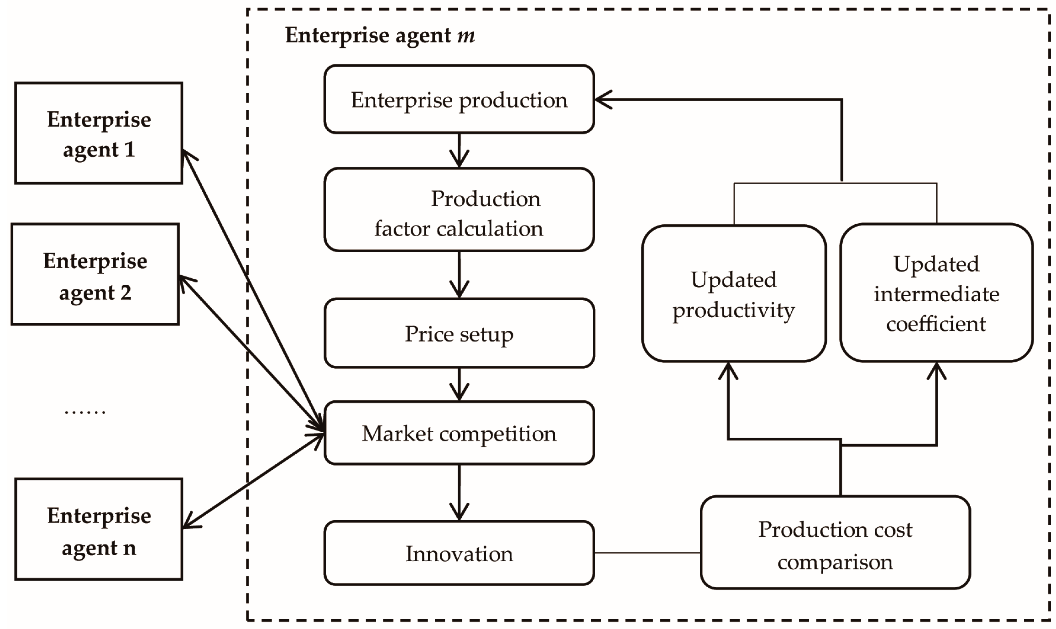
Therefore, with the modeling construction at the micro level, each enterprise agent is involved in a sequence of economic activities, including production, capital accumulation, market competition, and innovation. The flowchart of these activities is shown in Figure 2, along with the interactions with other agents. Enterprise agents interact with each other through market competition as reflected in agents’ market competitiveness and market share. A higher market share leads to a higher output, which in turn has an impact on the enterprise’s innovation. Driven by the enterprise’s innovation, a new intermediate coefficient matrix and a new productivity level are obtained. However, the adoption of the new intermediate coefficient matrix depends on whether it can reduce production costs. If it does, the agent will employ it adaptively.
2.3. Modeling Energy and Carbon Emissions
The objective of this module is to estimate future trends in China’s energy consumption, the structure of energy consumption, and carbon emissions. In accordance with the modeling of the economic system, we also use the bottom-up agent-based simulation to model energy and carbon emissions. Unlike the models in Section 2.1 and Section 2.2, which are derived mainly from Lorentz and Savona [24,25] with little modification, the entire model on energy and carbon emissions is our original work.
Following from evolutionary economics, enterprises’ R&D activities will not only promote improvements in the intermediate consumption coefficient and labor productivity, but also alter the technologies in energy consumption and carbon emissions. Generally speaking, both incremental innovations (in which minor extensions to existing processes or products are introduced without changing the current paradigm) and radical innovations (in which new techniques are used to produce a good) are important for technological change. However, we focus on incremental innovation from the perspective of evolutionary economics, because it is almost impossible for us to forecast an abrupt technological change induced by radical innovations. Our model therefore assumes that technologies change gradually. An enterprise’s successful innovation will alter its current energy consumption and carbon emissions in two ways: it will promote changes in the energy intensity of the enterprise, and it will also affect the energy consumption structure of the enterprise.
The total energy consumption of the enterprise () is determined by the total output of the enterprise () and the energy consumption intensity of the enterprise () in the current period:
The energy consumption intensity is affected by the enterprise’s innovation activities. When the innovation is successful, the energy consumption intensity will be affected by a random impact that observes a normal distribution. In addition, the enterprise will selectively update its energy consumption intensity in the direction of reducing energy intensity:
The enterprise’s energy consumption structure is affected by its innovation activities. In the base year, all of the enterprises in the same sector have the same energy consumption structure, which consists of consumption ratios of coal, petroleum, natural gas and electricity:
where represents the energy structure of enterprise i of sector k in the base year, and , , are, respectively, the consumption proportions of coal, petroleum, gas and electricity of sector k in the base year. In the evolution of the system, the evolution of the enterprise’s energy consumption structure varies because different innovation activities have different probabilities of success. When the innovation is successful, the enterprise’s energy structure transfers once under the action of the transfer matrix, which represents the enterprise’s energy structure advancing by one step:
where is the transfer matrix of the energy structure of sector k. Since the modeling time interval of our model is one year, the transfer matrix of energy structure will also be estimated based on annual energy structure change in China from 1991 to 2011 so as to meet the time scale requirement of the model.
The consumption of various energy sources of the sector, which is obtained by adding the enterprise’s total energy consumption and energy consumption structure, is as follows:
Thus, the sector’s total energy consumption (), proportion of various types of energy consumption (), and energy consumption structure () are as follows:
Carbon emissions are statistically analyzed at the sector level and calculated from the sector’s consumption of various energy sources and the carbon emission coefficients of various energy sources:
where represents the carbon dioxide emission factors of coal, petroleum and natural gas.
3. Data Processing
The 2000 input-output (IO) table of China, which is a 17-sector IO table, is taken as the basis for the initial values of parameters in the model, including intermediate consumption coefficients, final consumptions, and imports and exports data. The capital stocks, labor force, and capital elasticities at the sector level are from Xue [27]. In addition, the exogenous growth rates of sector consumption and export are averaged from the annual growth rate from 1997 through 2010; thus, we assume that China’s economy will keep growing at its current rate.
On the micro level, there are 500 enterprises in each of the 17 sectors. Due to the limitation of computation capacity, it is impossible to establish the same number of enterprises in each sector. The usual way of handling this issue is to set up a number of agents that can reflect the real characteristics of the real entities. For example, Basu et al. [28] established the ASPEN model simulating the US economy and set up 1000 households, 3 food firms, 2 automakers, 2 banks, etc. in which the number of each entity is not the same as in reality. Therefore, to present the sectoral attributes, the capital stock and labor force of each enterprise are averaged from the sector level at the time of initialization. In other words, enterprises from the same sector have identical initial capital stock and labor force, but initial capital stock and labor force vary across sectors. The initial energy intensity and energy consumption structure of each enterprise are identical to those of the sector level, which are deduced from the China Energy Statistical Yearbook 2000 [29]. Though enterprises have the same initial capital stock, labor force and other endowments, the enterprises’ innovation activities, which are influenced by a random shock as shown in Equation (22), will drive the different changes in such parameters, leading to the heterogeneity among enterprises.
4. Simulation Analyses
In the model, the enterprise’s innovation is impacted by normally distributed random impacts; therefore, the results of each simulation vary slightly. To fully consider the random impacts on the results, we simulated the model 50 times, and we analyzed the corresponding results of the 50 simulations using variance analyses and statistical tests of the differences between results. The p-values of the variance analysis were 1, indicating that the inter-group data showed no significant differences. Therefore, the average of the 50 sets of data can be used as representative results in the following analysis.
4.1. Model Verification
Before we estimated future energy consumption, we verified the reliability of the simulation results to determine whether the simulation reflects actual conditions; thus, the total energy consumption from 2001 to 2013 was simulated and compared with actual data. The results appear in Figure 3. The actual and simulated values are consistent and have a correlation coefficient of 0.99 and an analysis of variance (ANOVA) significance of 0.79. These results indicate that the simulation values accurately reflect the historical trajectories of energy consumption. They also suggest that the models are reliable and suitable for further studies on trends in energy consumption that are based on an evolutionary perspective, though they do not consider the possibility of abrupt technological changes.
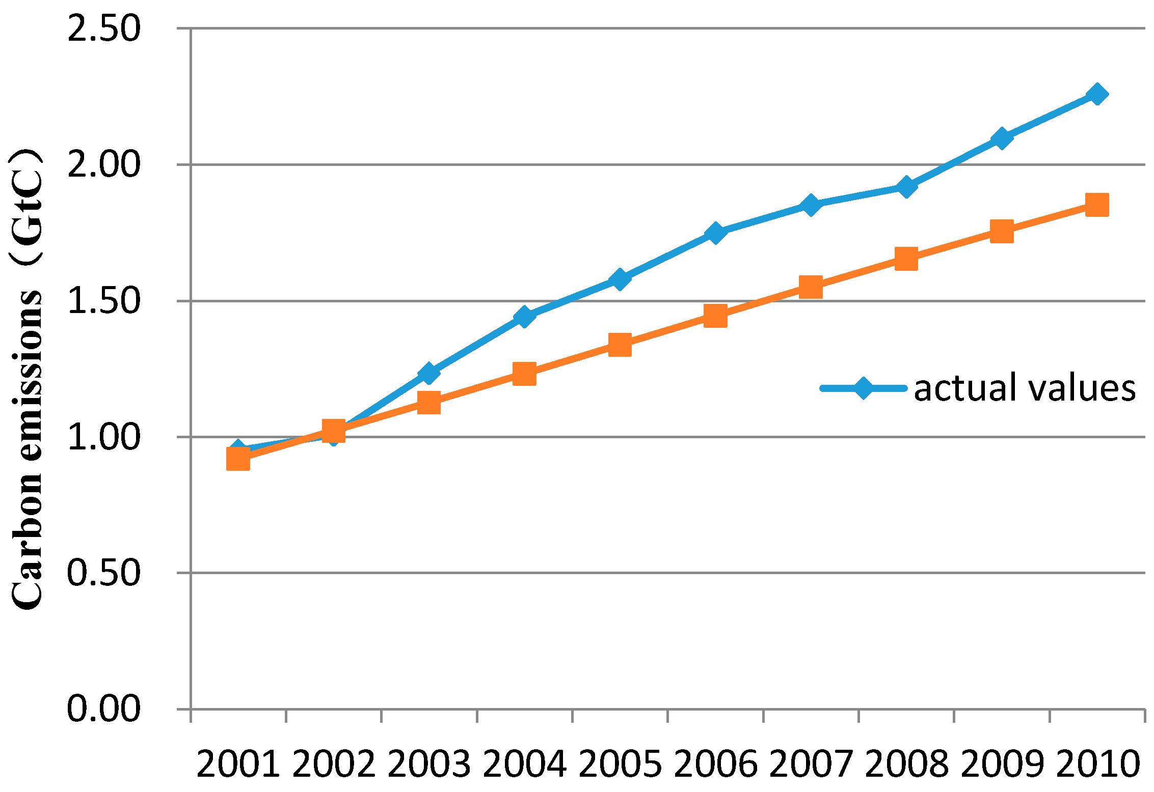
With the energy consumption projections, we can further analyze future carbon emissions. First, the 2001–2010 carbon emissions obtained by the simulation were calibrated with actual observation values (data obtained from the Carbon Dioxide Information Analysis Center, CDIAC, Oak Ridge, TN, USA). The results appear in Figure 4. The correlation coefficient between the actual values and simulated values is 0.99, with a variance test significance of 0.22; this indicates that there is no significant difference between the two data sets, and the model can reproduce the historical trajectories of the emissions. However, compared with the simulation on energy consumption, the simulation on carbon emissions shows a bigger simulation error when compared to actual data from 2001 to 2010. This error can be explained by the fit of the energy structure transfer matrix, which is an average of the status of the historical energy consumption from 1991 to 2011 by Markov chain. Over the last several years, the proportion of coal in the energy consumption structures of the agricultural and industrial sectors has been increasing, which is difficult to reflect in the Markov fitting; thus, it caused discrepancies in the energy structure that led to differences between the simulated carbon emissions and actual values.
4.2. Projections at the National Level
With the development of the economy and technological change driven by firms’ innovation, energy consumption and carbon emissions can be projected from the model.
Figure 5 shows the simulated trend of China’s energy consumption by 2050. Overall, it exhibits a trend of initial increases and then decreases. Energy consumption will peak in 2028 at 5295 Mtce (mega tonnes of coal equivalent), which is a 1.6-fold increase over the 2010 amount (3249 Mtce). Thereafter, the total energy consumption decreases yearly and will be approximately 3314 Mtce in 2050. We also calculated the annual energy consumption intensity per unit GDP by 2050. Results show that the simulated energy consumption intensity per unit GDP in China in 2010 is about 123 tce per million yuan. It will gradually decrease to 62.2 tce per million yuan in 2030 and 21.8 tce per million yuan in 2050. The averaged decline rate is about 3.8%.
Figure 6 shows trends in the sources of China’s energy by 2050. China’s sources of energy will change dramatically: the proportion of coal consumption will continue to decline from 62.9% in 2001 to approximately 41.2% in 2050; the proportion of petroleum consumption will increase slightly from 23% in 2001 to 36.7% in 2050; the proportion of natural gas will still be low, accounting for only 3.6% in 2050, but this is significantly more than the 2001 proportion of 1.9%; and the proportion of non-carbon energy consumption will grow to 18.4%.
Based on the calculations of economic growth and energy consumption, the trend of China’s carbon emissions by 2050 is obtained and shown in Figure 7. Carbon emissions will peak in 2027 at 2.77 GtC and then decline yearly until a value of 1.66 GtC is reached in 2050, a value that is almost equal to the 2005 level (1.58 GtC). Therefore, at the macro level, China’s peak emission year is around 2030, even a little bit earlier than 2030, meeting the INDC commitment China made at the 2015 Paris Climate Change Conference.
To provide a framework for comparison, Table 1 shows the carbon emissions peaks from other studies, as well as the methodology used in each study. Results show that most proposed emission peak years are between 2025 and 2040. The prediction presented in this study falls into the previously reported ranges.
4.3. Projections at the Industrial Level
R&D activities on the micro level can lead to a new intermediate coefficient matrix on the macro level, so that the industrial structure keeps evolving. Considering the three major industries (the primary industry, the secondary industry and the tertiary industry), we can obtain the proportion of each industry’s gross value added in GDP by summarizing the value added of each firm in the corresponding industry. Figure 8 shows changes in the proportions of China’s three major industries through 2050, reflecting the future evolution of industrial structures change in China. The proportions of the primary and secondary industries assume gradually decreasing trends, whereas the proportion of the tertiary industry assumes an increasing trend. By 2050, the proportions of the three major industries will be 3.3%, 31.7%, and 65%.
Due to the significant changes in China’s industrial structure, we are concerned about future energy consumption and carbon emissions at the industrial level. Figure 9 shows that industrial energy consumption also peaks by 2050. However, the peak year varies by industry. Specifically, the tertiary industry will experience its peak year in 2022, earlier than the other two industries, followed by the primary industry in 2023, while the secondary industry will have the latest peak year of energy consumption in 2029. It is obvious that due to energy intensive production in the secondary industry, its peak energy consumption is much later than the other two industries’ and even two years later than the national energy consumption peak. The peak energy consumption for the primary, secondary, and tertiary industries will be 53.71, 4770.95, and 512.87 Mtce, respectively. These results indicate remarkably high energy consumption in the secondary industry.
Moreover, because of differences in the production processes and technology levels in each of the major industries, the consumption structures of each of the energy sources also show differences. Table 2 shows the simulated energy consumption structures for each of the energy sources by 2050. The energy consumption of the primary industry is mainly non-carbon-based energy, which accounts for approximately 23.01%; the energy consumption of the secondary industry is mainly coal, which accounts for approximately 35.55%, with the highest consumption occurring in the machinery and equipment manufacturing sector; the energy consumption of the tertiary industry is mainly petroleum, which accounts for approximately 66.66%. Tertiary industries have a lower proportion of non-carbon energy consumption than primary or secondary industries. This is because the proportion of transportation and postal services accounts for only 3.3% of this sector (although the proportions of non-carbon energy consumption by all sectors except for transportation and postal services will reach approximately 34% in 2050). Thus, the overall proportion of the tertiary industry’s non-carbon energy consumption falls to merely 13.87%.
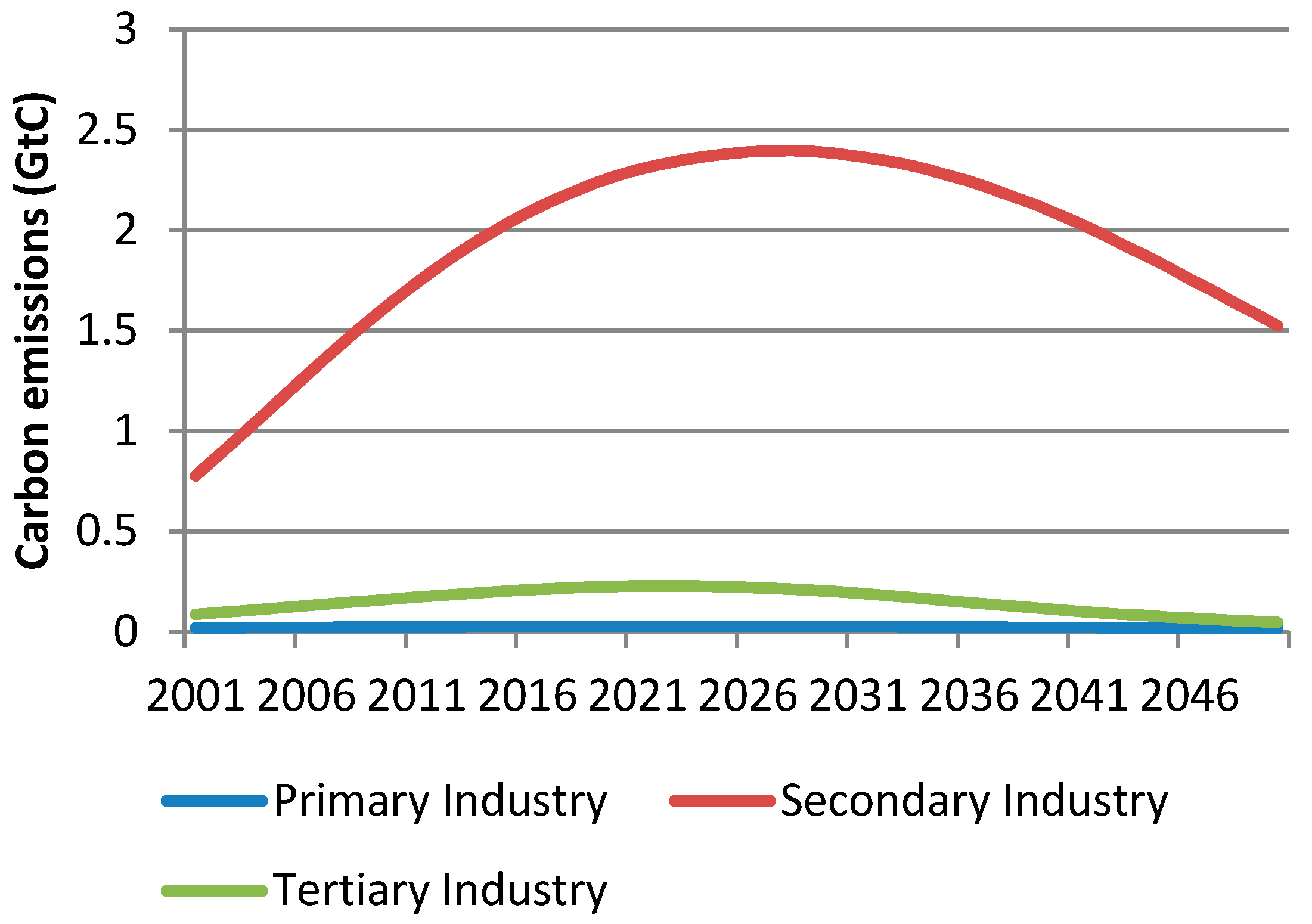
In addition to forecasting energy consumption forecasting, we also project carbon emissions at the industrial level. Figure 10 shows the results. The secondary industry continues to contribute most in China’s total emission through 2050. In 2027, the peak year of national emissions, emissions from the secondary industry account for 90% of the total due to the high proportion of fossil fuel consumption in this industry. With the influence of tremendous energy consumption, the secondary industry would reach its peak emission year in 2028 with emissions of 2.40 GtC, much later than the other two industries. The primary industry and the tertiary industry will reach their emission peaks together in 2022, with emissions of 0.024 GtC and 0.23 GtC, respectively.
4.4. Projections at the Sectoral Level
Section 4.3 notes the discrepancy between energy consumption trends at the industrial level and the national level; this discrepancy is also present in the carbon emission trends. Different industries have different peak years, because each industry has specific modes of production. Therefore, we examine how energy consumption and carbon emissions at the sectoral level differ from those at the national and industrial levels.
First, we explore the trend of sectoral development in China. Figure 11 shows the change in the sectors’ proportion of the national economy through 2050. Other services in the tertiary industry will develop rapidly in the future and account for approximately 29.5% of the sector in 2050. Simultaneously, the sectors of finance and insurance, utilities and residential services, commercial and catering businesses, etc. will also expand in the tertiary industry, with increasing proportions within the total economy. The proportions of the secondary industry sectors exhibit a gradually decreasing trend, and the sectors with the highest proportions in 2050 will be construction and machinery and equipment manufacturing, which will account for approximately 6% of the total economy. Change in sectoral development is consistent with change at industrial level: the tertiary industry expands, and the primary and secondary industries shrink.
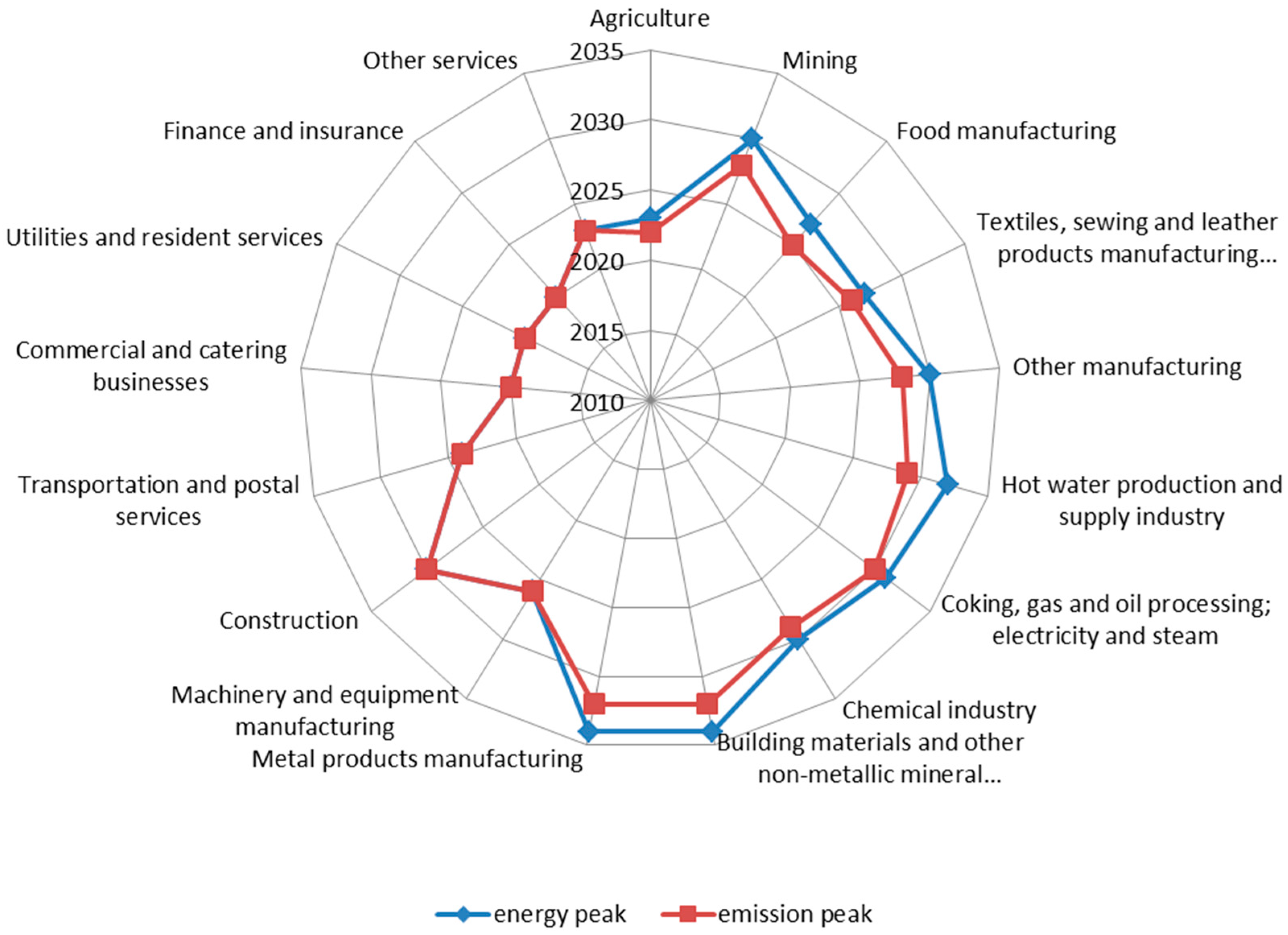
Meanwhile, the energy consumption and carbon emission peak years in each sector are abstracted and illustrated in Figure 12. There is significant variation across sectors. Sectors’ peak energy consumption is between 2020 and 2034, and peak carbon emission is between 2020 and 2032. Generally speaking, the sectoral carbon emission peak years arise prior to corresponding energy peak years, which is the same phenomenon we found at the national and industrial levels. The reason is that technological change reduces consumption of fossil fuel and increases consumption of non-fossil fuel, diminishing carbon emission from energy consumption. However, sectors in the tertiary industry are exceptional. They meet energy consumption peaks and carbon emission peaks in the same year despite the discrepancy in peak years by sector.
When comparing peak years across sectors, we find that the peak years of sectors in the primary and tertiary industries are earlier than those in the secondary industry, which are all prior to 2025. The first sectors achieving energy consumption peak and carbon emission peak come from the tertiary industry, including commercial and catering businesses, utilities and resident services, and finance and insurance. In these sectors, both energy and emissions peak in 2020. In agriculture, the sole sector in the primary industry, the energy consumption peak and carbon emission peak are the same as those at the industrial level: 2023 and 2022, respectively. Energy peaks for the sectors in the secondary industry appear from 2027 to 2034, about 5 to 10 years later than those of sectors in other industries. Building materials and other non-metallic mineral products manufacturing and metal products manufacturing are the two sectors with the latest energy peak year, 2034, while the first sector to reach peak energy consumption in the secondary industry is machinery and equipment manufacturing in 2026, followed by food manufacturing and textiles, sewing and leather products manufacturing industry in 2027. Though sectoral emission peaks occur before energy consumption peaks in the secondary industry, they still occur about 5 years later than in the primary industry and tertiary industries. Food manufacturing is the first sector in the secondary industry to reach emission peak, in 2025, which is 7 years earlier than emission peak of building materials and other non-metallic mineral products manufacturing and metal products manufacturing in 2032. These two sectors are the only ones to reach emission peak later than the 2030 target.
5. Conclusions and Discussion
Enterprise can change not only intermediate consumption patterns, but also the energy consumption structure and carbon emissions through technological progress promoted by its own innovative behavior. Therefore, it is necessary to use a typical bottom-up system when considering the future emission pathway in China. In this study, a 17-sector input-output model was integrated with an agent-based simulation, in which enterprise agents’ innovation affects industrial structure and energy demand at both the micro and macro levels and ultimately affects future trends in energy consumption and carbon emissions at multiple levels. The main results are as follows.
At the national level, China’s energy consumption will peak at 5295 Mtce in approximately 2028 and then fall to 3314 Mtce by 2050. The carbon emission at the national level will peak at 2.77 GtC in 2027 and decline to 1.66 GtC by 2050. Meanwhile, the dominant source of energy will be coal, which will account for 41.2% of consumption in 2050, while the proportion of petroleum consumption in 2050 will be 36.7%. The proportion of natural gas and non-carbon energy consumption will increase to 3.6% and 18.4%, respectively, by 2050.
At the industrial level, significant structural change will occur. By 2050, the proportions of the primary, secondary, and tertiary industries will be 3.3%, 31.7%, and 65%, respectively, indicating shrinkage in the primary and secondary industries and expansion in the tertiary industry. The energy consumption peaks for the primary, secondary, and tertiary industries will be reached in 2023, 2029, and 2022, respectively; while their carbon emission peaks will occur in 2022, 2022, and 2028. The energy consumption and carbon emission peak years of the secondary industry are both later than those at the national level, revealing a pressure for the secondary industry to curb its emission induced by its heavy dependence on fossil fuel energy consumption.
At the sectoral level, sectors’ proportions in the national economy also keep changing through 2050. Other services in the tertiary industry will develop rapidly and account for the greatest proportion of approximately 29.5% in 2050. Construction and machinery and equipment manufacturing will make up the largest part of the secondary industry by 2050. Due to the evolution of sectoral development, there is a remarkable discrepancy in energy consumption and carbon emission among sectors. Sectors’ peak energy consumption occurs between 2020 and 2034, and their peak carbon emissions occurs between 2020 and 2032. The first sectors to achieve peak energy consumption and peak carbon emission come from the tertiary industry, including commercial and catering businesses, utilities and resident services, and finance and insurance, which peak in 2020 for both energy and emissions. We see 5- to 10-year and 5-year lags, respectively, for the energy consumption peaks and carbon emissions peaks of sectors in the secondary industries as compared to sectors from the other two industries. Together, building materials and other non-metallic mineral products manufacturing and metal products manufacturing will experience the latest energy consumption peak and emission peak in 2034 and 2032, respectively.
This study demonstrates that agent-based simulation, in which micro behaviors can be integrated with the evolution of macroeconomic structures, is a powerful and suitable tool to apply in the field of energy and emission forecasting. However, the model we present in this paper is still preliminary, and more research is needed to improve it. For instance, in our model, enterprises’ innovation is costless, which may not be the case in reality. The model also ignores enterprises’ knowledge accumulation, which is necessary to represent different capabilities in innovation. Finally, knowledge diffusion and spillovers should be considered in future improvements to the model.
Acknowledgments
This work is supported by the National key R&D plan Program of China No. 2016YFA0602702 and the National Science Foundation of China (Grant No. 41501127).
Author Contributions
Z.W. and J.W. conceived and designed the model; J.W. developed the model and analyzed the data; J.W. and R.M. wrote the paper.
Conflicts of Interest
The authors declare no conflict of interest.
References
- Aydin, G. Modeling of energy consumption based on economic and demographic factors: The case of Turkey with projections. Renew. Sustain. Energy Rev. 2014, 35, 382–389. [Google Scholar] [CrossRef]
- Suganthi, L.; Anand, A. Samuel Energy models for demand forecasting—A review. Renew. Sustain. Energy Rev. 2012, 16, 1223–1240. [Google Scholar] [CrossRef]
- Parajuli, R.; Østergaard, P.A.; Dalgaard, T.; Pokharel, G.R. Energy consumption projection of Nepal: An econometric approach. Renew. Energy 2014, 63, 432–444. [Google Scholar] [CrossRef]
- Auffhammer, M.; Carson, R.T. Forecasting the path of China’s CO2 emissions using province-level information. J. Environ. Econ. Manag. 2008, 55, 229–247. [Google Scholar] [CrossRef]
- Yuan, J.; Xu, Y.; Hu, Z.; Zhao, C.; Xiong, M.; Guo, J. Peak energy consumption and CO2 emissions in China. Energy Policy 2014, 68, 508–523. [Google Scholar] [CrossRef]
- Uzlu, E.; Kankal, M.; Akpinar, A.; Dede, T. Estimates of energy consumption in Turkey using neural networks with the teaching—Learning-based optimization algorithm. Energy 2014, 75, 295–303. [Google Scholar] [CrossRef]
- Ekonomou, L. Greek long-term energy consumption prediction using artificial neural networks. Energy 2010, 35, 512–517. [Google Scholar] [CrossRef]
- Ceylan, H.; Ozturk, H.K. Estimating energy demand of Turkey based on economic indicators using genetic algorithm approach. Energy Convers. Manag. 2004, 45, 2525–2537. [Google Scholar] [CrossRef]
- Wing, S.; Eckaus, R.S. The implications of historical decline in US energy intensity for long-run CO2 emission projections. Energy Policy 2007, 35, 5267–5286. [Google Scholar] [CrossRef]
- Wang, Z.; Zhu, Y.; Liu, C.; Ma, X. Integrated projection of carbon emission for China under optimal economic growth path. Acta Geogr. Sin. 2010, 65, 1559–1568. [Google Scholar]
- Vaillancourt, K.; Alcocer, Y.; Bahn, O.; Fertel, C.; Frenette, E.; Garbouj, H.; Kanudia, A.; Labriet, M.; Loulou, R.; Marcy, A.; et al. A Canadian 2050 energy outlook: Analysis with the multi-regional model TIMES-Canada. Appl. Energy 2014, 132, 56–65. [Google Scholar] [CrossRef]
- Desmarchelier, B.; Djellal, F.; Gallouj, F. Environmental policies and eco-innovations by service firms: An agent-based model. Technol. Forecast. Soc. Chang. 2013, 80, 1395–1408. [Google Scholar] [CrossRef]
- Lee, T.; Yao, R.; Coker, P. An analysis of UK policies for domestic energy reduction using an agent based tool. Energy Policy 2014, 66, 267–279. [Google Scholar] [CrossRef]
- Gerst, M.D.; Wang, P.; Rovenini, A.; Fagiolo, G.; Dosi, G.; Howarth, R.B.; Borsuk, M.E. Agent-based modeling of climate policy: An introduction to the ENGAGE multi-level model framework. Environ. Modell. Softw. 2013, 44, 62–75. [Google Scholar] [CrossRef]
- Mialhe, F.; Becu, N.; Gunnell, Y. An agent-based model for analyzing land use dynamics in response to farmer behaviour and environmental change in the Pampanga delta (Philippines). Agric. Ecosyst. Environ. 2012, 161, 55–69. [Google Scholar] [CrossRef]
- Nannen, V.; Van den Bergh, J.; Eiben, A.E. Impact of environmental dynamics on economic evolution: A stylized agent-based policy analysis. Technol. Forecast. Soc. Chang. 2013, 80, 329–350. [Google Scholar] [CrossRef]
- Macal, C.M.; North, M.J. Tutorial on agent-based modeling and simulation. J. Simul. 2010, 4, 151–162. [Google Scholar] [CrossRef]
- Azar, E.; Menassa, C.C. Agent-based modeling of occupants and their impact on energy use in commercial buildings. J. Comput. Civ. Eng. 2011, 26, 506–518. [Google Scholar] [CrossRef]
- De Hann, P.; Mueller, M.G.; Scholz, R.W. How much do incentives affect car purchase? Agent-based microsimulation of customer choice of new cars- Part II: Forecasting effects of feebates based on energy-efficiency. Energy Policy 2009, 37, 1083–1094. [Google Scholar] [CrossRef]
- Lin, H.; Wang, Q.; Wang, Y.; Wennerstern, R.; Sun, Q. Agent-based modeling of electricity consumption in an office building under a tiered pricing mechanism. Energy Procedia 2016, 104, 329–335. [Google Scholar] [CrossRef]
- Chappin, E.J.L. Carbon Dioxide Emission Trade Impact on Power Generation Portfolio: Agent-based Modelling to Elucidate Influences of Emission Trading on Investments in Dutch Electricity Generation. Master’s Thesis, Delft University of Technology, Delft, The Netherlands, 2006. [Google Scholar]
- Tang, L.; Wu, J.; Yu, L.; Bao, Q. Carbon emissions trading scheme exploration in China: A multi-agent-based model. Energy Policy 2015, 81, 152–169. [Google Scholar] [CrossRef]
- Zhu, Q.; Duan, K.; Wu, J.; Zheng, W. Agent-based modeling of global carbon trading and its policy implications for China in the Post-Kyoto Era. Emerg. Mark. Financ. Trade 2016, 52, 1348–1360. [Google Scholar] [CrossRef]
- Lorentz, A.; Savona, M. Evolutionary micro-dynamics and changes in the economic structure. J. Evol. Econ. 2008, 18, 389–412. [Google Scholar] [CrossRef]
- Lorentz, A.; Savona, M. Structural Change and Business cycles: An Evolutionary Approach; Papers on Economics and Evolution 21; Philipps University Marburg, Department of Geography: Marburg, Germany, 2010. [Google Scholar]
- Gong, Y.; Gu, G.; Liu, C.; Wang, Z. Chinese industry structure evolution driven by innovation. Stud. Sci. Sci. 2013, 31, 1252–1259. [Google Scholar]
- Xue, J. CGE Modelling on China’s Macroeconomy; Institute of Policy and Management, Chinese Academy of Sciences: Beijing, China, 2006. [Google Scholar]
- Basu, N.; Pryor, R.; Quint, T. ASPEN: A microsimulation model of the economy. Comput. Econ. 1998, 12, 223–241. [Google Scholar] [CrossRef]
- Department of Energy Statistics, National Bureau of Statistics. China Energy Statistical Yearbook 2000; China Statistics Press: Beijing, China, 2000.
- Zhu, Y.; Wang, Z.; Pang, L.; Zou, X. Simulation on China’s economy and prediction on Energy consumption and carbon emission under optimal growth path. Acta Geogr. Sin. 2009, 64, 935–944. [Google Scholar]
- Jiang, K.; Hu, X. Low-Carbon Scenarios by 2050 in China//Research Team on China’s Energy Use and Carbon Emission; 2050 China Energy and CO2 Emissions Report; Science Press: Beijing, China, 2009; pp. 753–819. [Google Scholar]
- Du, Q.; Chen, Q.; Lu, N. Forecast of China’s carbon emissions based on modified IPAT model. Acta Sci. Circumst. 2012, 32, 2294–2302. [Google Scholar]
- Yue, P.; Wang, S.; Zhu, J.; Fang, J. 2050 carbon emissions projection for China—Carbon emissions and social development, IV. Acta Sci. Nat. Univ. Pekin. 2010, 46, 517–524. [Google Scholar]
- Qu, S.; Guo, C. Forecast of China’s carbon emissions based on STIRPAT model. China Popul. Res. Environ. 2010, 20, 10–15. [Google Scholar]
- Liu, C.; Chen, Z.; Qu, S. China’s Emission Peak and Its Industrialization Process; Annual Report on Actions to Address Climate Change; Wang, W., Zheng, G., Eds.; Social Sciences Academic Press: Beijing, China, 2014; pp. 139–150. [Google Scholar]
- Lu, Y. China’s Emission Peak and Its Residential Consumption; Annual Report on Actions to Address Climate Change; Wang, W., Zheng, G., Eds.; Social Sciences Academic Press: Beijing, China, 2014; pp. 183–191. [Google Scholar]
Figure 1.
Interactions between macro and micro levels.

Figure 2.
The activities flowchart of an individual enterprise agent and its interaction with other agents.
Figure 2.
The activities flowchart of an individual enterprise agent and its interaction with other agents.

Figure 3.
Comparison of the simulated values and actual values of energy consumption from 2001 to 2013 (Mtce: mega tonnes of coal equivalent).
Figure 3.
Comparison of the simulated values and actual values of energy consumption from 2001 to 2013 (Mtce: mega tonnes of coal equivalent).
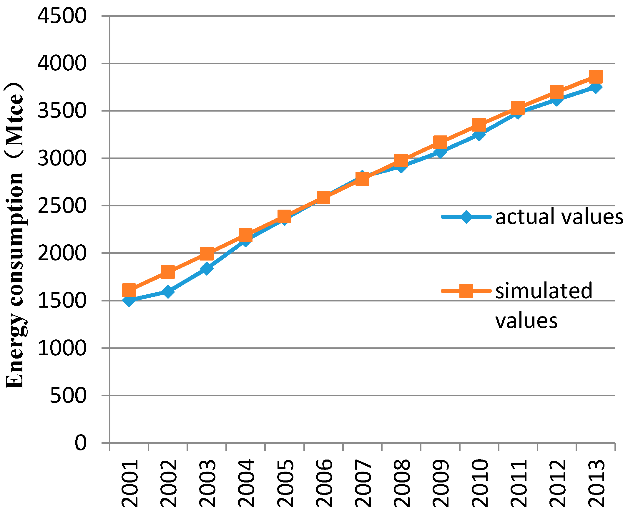
Figure 4.
Comparison of simulated and actual values of carbon emissions from 2001 to 2010 (GtC: Gigatonnes of Carbon).
Figure 4.
Comparison of simulated and actual values of carbon emissions from 2001 to 2010 (GtC: Gigatonnes of Carbon).

Figure 5.
China’s total energy consumption trend by 2050.
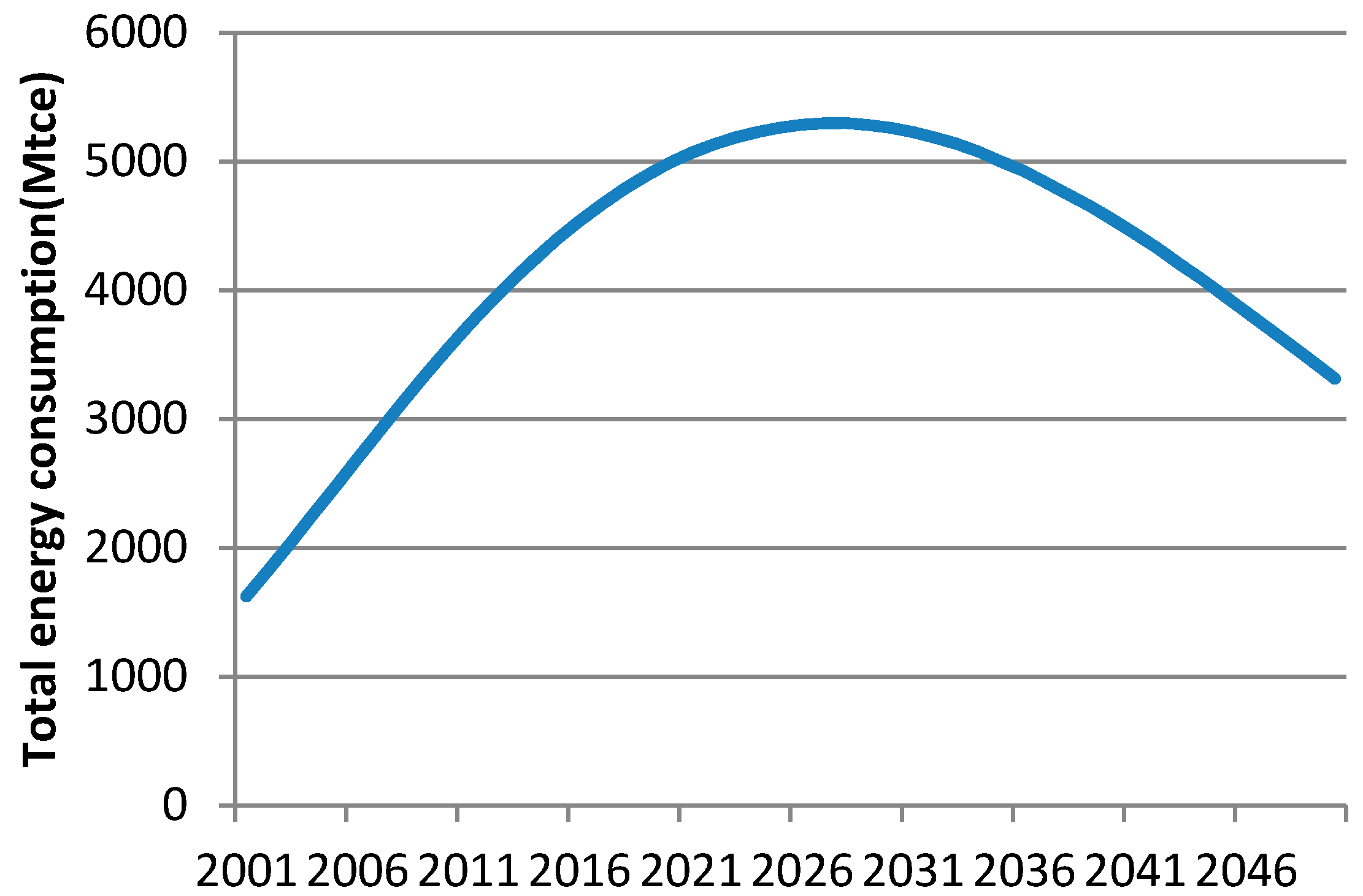
Figure 6.
China’s energy consumption structure change trend by 2050.
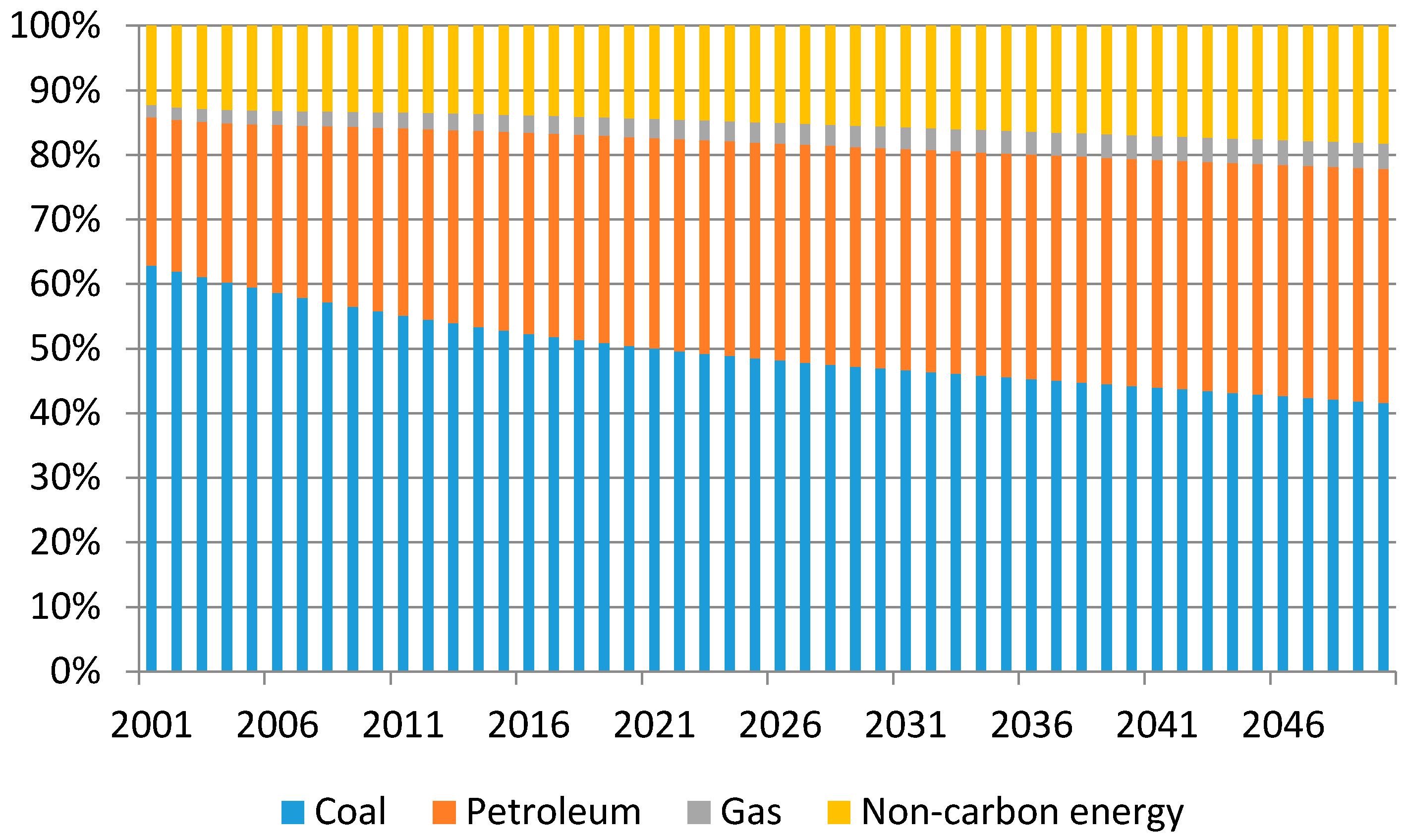
Figure 7.
Trend of China’s carbon emissions by 2050.
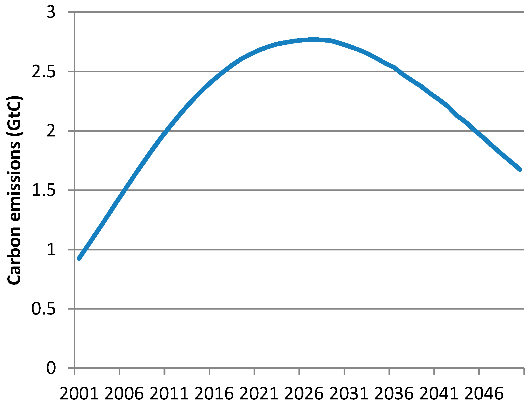
Figure 8.
Evolution of the proportion of China’s three main industries by 2050.
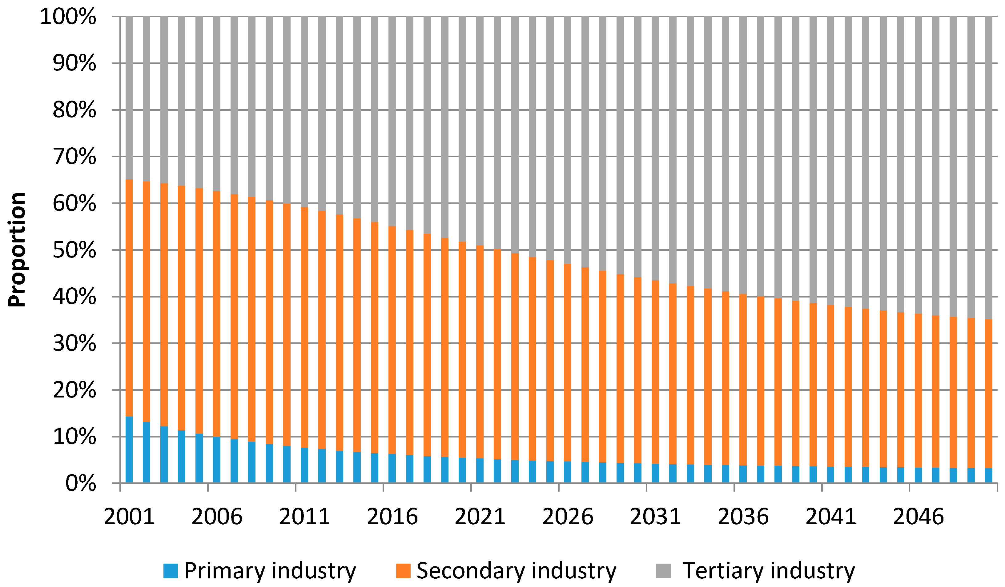
Figure 9.
Trend of energy consumption at the industrial level.
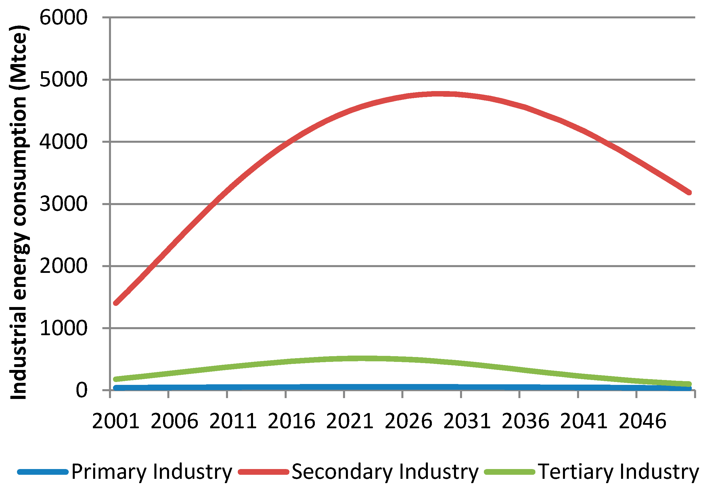
Figure 10.
Trend of carbon emissions at the industrial level.

Figure 11.
Evolution of China’s industrial structure through 2050.
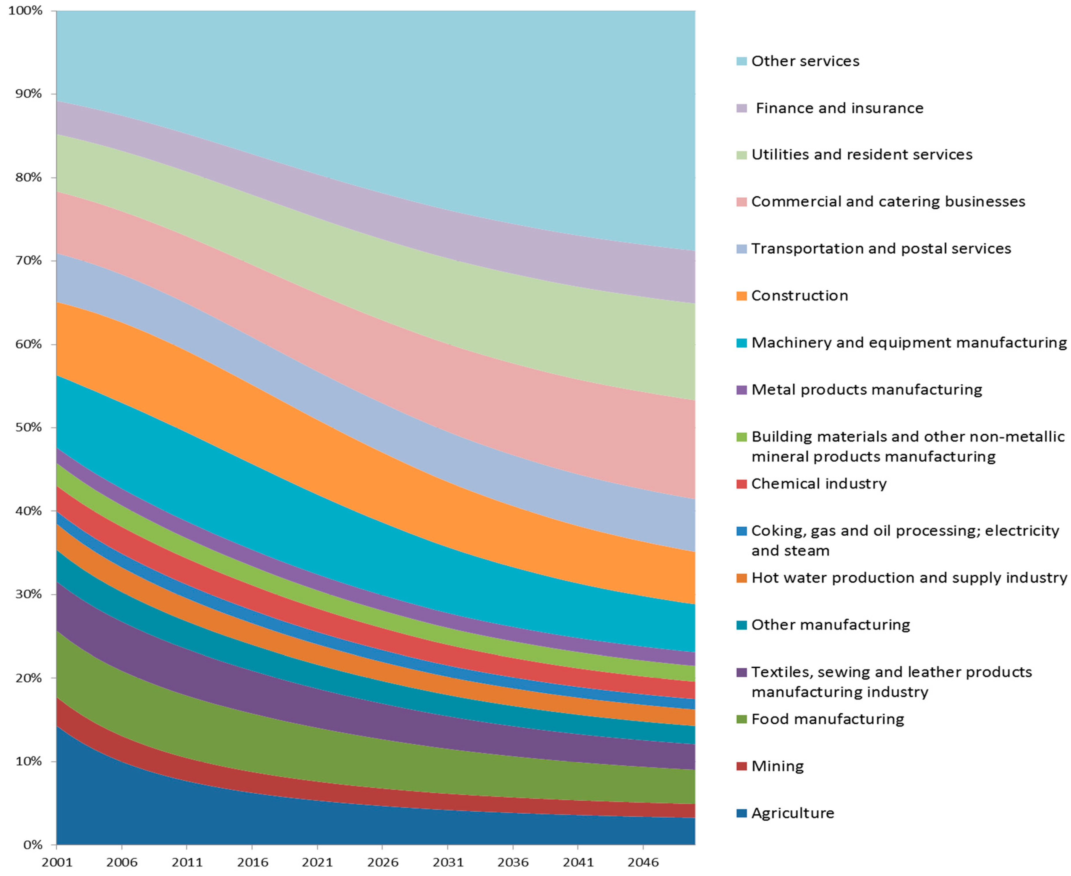
Figure 12.
The peak years of energy consumption and carbon emissions at the sectoral level.


Table 1.
Comparisons of the peak years of carbon emissions proposed by different studies.
| Authors | Peak Year | Peak Value | Method Used |
|---|---|---|---|
| Zhu et al. [30] | 2040 | 3.8 GtC | Economic optimal growth model |
| Jiang and Hu [31] | 2030–2040 | - a | Technology model |
| Wang et al. [10] | 2031 | 2.6 GtC | Economic optimal growth model |
| Du et al. [32] | 2030 | 3.68 GtC | IPAT model |
| Yue et al. [33] | 2035 | 4.4 GtC | Trend extrapolation model |
| Qu and Guo [34] | 2020–2045 | - a | STIRPAT model |
| Yuan et al. [5] | 2030–2035 | 2.5 GtC | Kaya model |
| Liu et al. [35] | 2025–2030 | - a | Kaya model |
| Lu [36] | Approximately 2025 | 2.86 GtC | Trend extrapolation model |
a No specific peak data provided.
Table 2.
Energy consumption structure of various industries in 2050.
| Coal | Petroleum | Gas | Non-Carbon Energy | Total | |
|---|---|---|---|---|---|
| Primary industry | 17.81% | 59.06% | 0.02% | 23.01% | 100.00% |
| Secondary industry | 42.54% | 35.55% | 3.39% | 18.52% | 100.00% |
| Tertiary industry | 6.68% | 66.66% | 12.79% | 13.87% | 100.00% |
© 2017 by the authors. Licensee MDPI, Basel, Switzerland. This article is an open access article distributed under the terms and conditions of the Creative Commons Attribution (CC BY) license (http://creativecommons.org/licenses/by/4.0/).
Share and Cite
MDPI and ACS Style
Wu, J.; Mohamed, R.; Wang, Z. An Agent-Based Model to Project China’s Energy Consumption and Carbon Emission Peaks at Multiple Levels. Sustainability 2017, 9, 893. https://doi.org/10.3390/su9060893
AMA Style
Wu J, Mohamed R, Wang Z. An Agent-Based Model to Project China’s Energy Consumption and Carbon Emission Peaks at Multiple Levels. Sustainability. 2017; 9(6):893. https://doi.org/10.3390/su9060893
Chicago/Turabian StyleWu, Jing, Rayman Mohamed, and Zheng Wang. 2017. "An Agent-Based Model to Project China’s Energy Consumption and Carbon Emission Peaks at Multiple Levels" Sustainability 9, no. 6: 893. https://doi.org/10.3390/su9060893
Note that from the first issue of 2016, this journal uses article numbers instead of page numbers. See further details here.