
Sustainability from the Occurrence of Critical Dynamic Power System Blackout Determined by Using the Stochastic Event Tree Technique

Faculty of Electrical Engineering, Universiti Teknologi MARA, 40450 Shah Alam, Selangor, Malaysia
*
Author to whom correspondence should be addressed.
Sustainability 2017, 9(6), 941; https://doi.org/10.3390/su9060941
Submission received: 26 March 2017
/
Revised: 28 May 2017
/
Accepted: 31 May 2017
/
Published: 3 June 2017
(This article belongs to the Special Issue Sustainable Electric Power Systems Research)
Abstract
:With the advent of advanced technology in smart grid, the implementation of renewable energy in a stressed and complicated power system operation, aggravated by a competitive electricity market and critical system contingencies, this will inflict higher probabilities of the occurrence of a severe dynamic power system blackout. This paper presents the proposed stochastic event tree technique used to assess the sustainability against the occurrence of dynamic power system blackout emanating from implication of critical system contingencies such as the rapid increase in total loading condition and sensitive initial transmission line tripping. An extensive analysis of dynamic power system blackout has been carried out in a case study of the following power systems: IEEE RTS-79 and IEEE RTS-96. The findings have shown that the total loading conditions and sensitive transmission lines need to be given full attention by the utility to prevent the occurrence of dynamic power system blackout.
1. Introduction
Congestion management is a challenging task for an Independent System Operator (ISO) that has the responsibility to ensure effectiveness and safety in the operation of a deregulated power system. This is because the system is increasingly stressed because of adverse impact from a competitive electricity market augmented by the uncertain operation of smart grid and renewable energy. Consequently, several implications of sensitive transmission line tripping and severe total loading condition include occurrence of severe blackouts being likely to be experienced by a deregulated power system operation. Therefore, it is imperative to seek a solution providing an early detection of sensitive transmission line and severe total loading condition in such a way that preventive action can be realized to prevent the emergence of power system blackout. The dynamic response of a system plays an imperative role in the analysis of power system security, especially when it entails a power system blackout, which is usually caused by the impact of enormous and unforeseen faults, unexpected generation and load outages, and abrupt increment of loads [1].
Several studies on the static power system blackout analysis have been deliberated in recent literature. The probability distribution function (PDF) of system blackout for the Oak Ridge-PSERC-Alaska (OPA) power system model was examined and investigated based on the adjustment of loading condition [2,3,4,5]. This method uses the DC power flow solution and the linear programming method to reduce the cost function of power system blackout. The obtained PDF of OPA power system blackout is then used to perform a risk assessment of system blackout for a different power system model. However, the disadvantage of using the OPA power system model is that only a small number of nodes are required to construct a network model [6]. This is because the proposed method may cause exponential divergence of PDF for other types of large power system and result in inaccurate risk assessment for power system blackout. Another approach adopted to study the power system blackout phenomena is the CASCADE technique [4,5,7]. CASCADE technique is used to assess a general qualitative behavior that may be present in power system cascading failures. The acquired outcome will be risk assessment of a power system blackout that is purported to be relatively analogous to a small interruption. From the literature survey, it is noteworthy that the dynamic power system blackout has not been explored particularly for the determination of sensitive transmission lines and severe total loading conditions.
This paper will discuss the determination of sensitive transmission lines and severe total loading conditions as a result of a dynamic power system blackout caused by an initial tripping of transmission line. The dynamic power system blackout can be regarded as the propagation of system component tripping agitated by either an overloaded transmission line or violation of a synchronous generator rotor angle and frequency limits. Efficacy of the proposed stochastic event tree technique utilized in the risk assessment of a dynamic power system blackout is confirmed via the case study of the following power systems: IEEE RTS-RTS79 and IEEE RTS-96. It is imperative for the proposed stochastic event tree technique to consider the critical clearing time (CCT) of a protection relay, generator rotor angle, forced outage rate (FOR) of a generator, and simultaneous tripping of exposed transmission lines and generators in such a way that it is the basic approach that critically needs to be considered in the risk assessment of dynamic power system blackout. The abovementioned approach has not been considered and discussed in previous literature even though the stochastic event tree method has been used in the analysis of dynamic power system blackout [8,9,10]. As a compendium for this section, dynamic power system blackout should be assessed regularly by the utility in such a way that it will be useful to improvise an early stage of preventive action by identifying the sensitive transmission lines and severe total loading conditions.
2. Research Methodology
This section will discuss the One Machine Infinite Bus (OMIB) required to simplify a large scale of dynamic equivalent multi-machine system model. The OMIB equivalent model of a multi-machine system is implemented directly to determine the critical clearing time (CCT), , required in the risk assessment of a dynamic power system blackout for the determination of sensitive transmission lines and severity of loading conditions. A detail explanation and derivation of OMIB can be obtained by referring to the discussion in [11,12,13].
2.1. One Machine Infinite Bus (OMIB) Rotor Angle during Pre-Fault Condition
The main concept of one machine infinite bus (OMIB) model refers to a single machine equivalent (SIME) method that is carried out to simplify the computationally challenging factor of a multi-machine system with non-linear time domain simulation [14,15,16]. The following procedure will elaborate on the determination of rotor angle associated with the OMIB.
- Distinguish between the critical, cm, and non-critical, ncm, machines identified with regards to the threshold, as explicated in Equation (1). The determination of critical and non-critical machines (Equation (1)) has been introduced in [17]. In particular, Li et al. [17] elucidated that the angular deviation of each generator with respect to the center of inertia (COI) can be used to overcome the difficulties in identifying the critical and non-critical machines. The same concept has also been implemented and discussed in [18,19,20]. In Equation (1), the signifies that an accelerating power occurred in the critical machines. On the other hand, the implies that a decelerating power incurred in the non-critical machines.wherewhere H is the inertia driven by a synchronous machine (per unit); and G is the total number of generating units.
- Use Equations (8)–(10) and (14) to calculate the , , and , respectively. The above-mentioned equations are derived from Equation (4), which is the initial formulation of OMIB motion or swing. All of the parameters given below should be changed into a standard per-unit (p.u.) value to ease calculation in relation to the OMIB.whereis the generating unit’s mechanical input power; is the real electric power output of generator; frated is the rated frequency operated in a system; Mcm is the total inertia for cm represented by ; Mcnm is the total inertia for ncm represented by ; and M is the OMIB inertia determined by 2×H.
- Simultaneously, the OMIB motion or swing equation is simplified by further derivation of Equation (4).where
- In the Transient Stability Assessment (TSA) of a multi-machine, the pre-fault condition is performed to obtain the information of Pm, generator voltage () and shunt conductance (G), indispensible for Equations (8)–(13). The G is originated from the bus admittance matrix of Ynk constructed without the composition of faulted transmission line and faulted bus. Wherein, k is the bus number. Simultaneously, Equation (14) is used to determine the OMIB rotor angle during pre-fault condition, .
The following section will explain the importance of for specifying the critical clearing time (CCT) for the tripping of generators and transmission lines.
2.2. Determination of Critical Clearing Time for One Machine Connected to an Infinite Bus
Emphasis on the improvement of CCT to corroborate the new changes occurring in a power system is important so that it always operates in a stable condition, especially during the unanticipated fault situation. Duong et al. has discussed a new CCT determination referring to a fault condition occurring in a power system taking into account the operation of wind turbines based squirrel-cage induction generator [21]. Subsequent improvement of CCT has been made to ensure the low voltage ride through type of fault does not infringe the secure operation of a power system connected with the wind turbines based double-fed induction generator [22].
This implies that it is imperative to perform a transient stability analysis, as this is required to stipulate an accurate critical clearing time (CCT) implemented in a protection relay for disconnecting the faulted transmission line so that the healthy system remains transiently stable. During the fault interval, the implication of transmission line tripping is that it will cause a generator to refrain from dispatching its electric power to an infinite bus. As a result, the generator does not provide any electrical output power (Pe) and is the reason Equation (4) simplifies to Equation (15). Therefore, Equation (17) is utilized to attain the OMIB critical clearing time, .
Further expansion of Equation (15) yields Equation (16).
Equation (17) is the OMIB critical clearing time () derived from Equation (16). The analytical calculation of has been proven and discussed thoroughly in [23,24,25].
where
This signifies that OMIB is further derived to obtain formulation of . The based OMIB is useful as a standard reference to specify the CCT for all protection relays in a power system consisting with multi-machine or numerous generators. The importance of OMIB via towards the power system operating condition comprising multi-machine or numerous generators has also been discussed and implemented in [24]. Nevertheless, this paper proposes a new approach to analyze the condition of dynamic power system blackout by taking into account the transmission lines and/or generators tripping due to the protection relay operation at the time interval of CCT specified by the based OMIB. This will be discussed in Section 2.3.
The procedure given below explains in detail the algorithm of the OMIB critical clearing time, .
- Perform a fault at the selected bus inflicting the affected transmission line tripping.
- Execute the TSA so the Ynk can be determined during the pre-fault and fault conditions.
- Exert and Pm in Equation (14) to determine . The Ynk obtained in Step (2) is used to determine Pm during the pre-fault condition.
- Inflict , and in Equation (18) to determine . The and during post-fault condition are attained from Equations (8) and (10), respectively.
- Use Equation (17) to calculate for the affected transmission line selected in Step (1); requires information regarding and as well as , which is acquired from Steps (7) and (14), respectively. Compute for the subsequent affected transmission line by repeating Steps (1)–(5).
- Stipulate a standard CCT by referring to the smallest and impose it as a reference for all protection relays.
2.3. Evaluation of Sensitive Transmission Lines and Total Loading Condition
In a deregulated power system, an inaccurate operation in a protection relay system may cause a proliferation of major system disturbances and eventually lead to a power system blackout [26,27,28]. This happens because a hidden failure, regarded as an undetected or unidentified defect of a protection relay, causes a false tripping during a normal situation or an exposure to the disturbances from other components in the system [26,27,28]. The hidden failure probability of pHF = 8 × 10⁻⁷, pHF = 1 × 10–12 and pHF = 1 × 10⁻², introduced as the three case studies in [29], are subsequently utilized in this section to assess its implication against the probability of dynamic power system blackout. This signifies that the analysis executed based on the proposed approach is contradictory with the analysis undertaken in [29] whereby the probability of static power system blackout is determined based on the three case studies of pHF. With regards to every case study, the procedure of stochastic event tree will explain in detail the risk assessment by means of average probability of dynamic power system blackout posed by the occurrence of initial transmission line tripping. The information is indispensable for the estimation of severe transmission lines and total loading conditions.
- Introduce a power system blackout attributed by a stress system condition arising from an increase of 10% on the total loading condition.
- Specify the for the entire protection relays as discussed in Section 2.2.
- Select a transmission line for tripping at an initial event tree, i. Execute the power flow solution and TSA of multi-machine considering the transmission line tripping at an initial event tree, i.
- Determine the probability of incorrect tripping (pHF) [30] and forced outage rate (FOR) of all exposed transmission lines and exposed generators, respectively. The exposed transmission lines and exposed generators can be described as the system components connected adjacent to the transmission line tripping. The historical information of protection relay hidden failure is used to calculate the pHF [30]. However, the hidden failure probability of pHF = 8 × 10⁻⁷, pHF = 1 × 10⁻¹² and pHF = 1 × 10⁻² obtained in [29] will be used in the analysis.
- Randomly or stochastically exert the tripping of exposed transmission lines and/or exposed generators prior to the attainment of limit imminent in the branch event tree j. The tripping of exposed transmission lines and exposed generators refer to the randomly or stochastically generated probability that infringe the pHF limit [30]; and FOR limit as well as frequency limit or rotor angle limit, respectively.
- Record the pHF and qHF =1 − pHF of exposed transmission lines, the FOR and 1-FOR of exposed generators and the total random or stochastic tripping, Z, in the branch event tree j. The qHF can be defined as the probability of exposed transmission line not encountering the random tripping event.
- Use Equation (20) to calculate the conditional probability of tripping (PTj) during branch event tree, j.where is the pHF for the random or stochastic tripping of exposed transmission lines, or the FOR of random or stochastic tripping of exposed generators; and is the qHF for non-tripping of exposed transmission lines, or the 1-FOR of non-tripping of exposed generators.
- Run the power flow solution and TSA of multi-machine system.
- Calculate PTj using Equation (20) for the ensuing branch event tree j by repeating Steps (4)–(8).
- Determine , which is the product of tripping probability, using Equation (21).
- Determine , which is the average probability of sequential random or stochastic tripping, using Equation (22) by repeating Steps (4)–(10) for KP = 1000 times.
- Acquire for the subsequent tripping of transmission line at initial event tree, i, by executing Steps (3)–(11).
- Execute Steps (1)–(15) to determine for every increment of total loading condition until its maximum level is reached.
- Calculate , which is the estimated average probability of dynamic power system blackout, using Equation (23).where L is the total steps required for the increase of total loading condition.
- Distinguish the sensitive transmission lines during the initial tripping or initial event tree by means of significant increase in the value.
- Calculate , which is the estimated average probability of dynamic power system blackout, using Equation (24).where I is the total number of transmission lines.
- Arrange the in ascending order to determine the critical dynamic power system blackout that is caused by the severity of total loading condition. Distinguish the severity of total loading conditions inflicting a critical dynamic power system blackout by means of significant increase in the value.
3. Results
This section will discuss the sustainability of power system operation for the case studies of IEEE RTS-79 and IEEE RTS-96 under the perspective of risk assessment in dynamic power system blackout. IEEE RTS-79 and IEEE RTS-96 were designed based on the real parameters and pragmatic components acquired based on consensus from power system experts. Usually, these systems are used as a case study for benchmarking the findings of similar study obtained based on different methods or approaches suggested by researchers. Similarly, the initiative highlighted in this manuscript is the implementation of IEEE RTS-79 and IEEE RTS-96 as case studies, which is sufficient to prove the proposed method can be used to determine the risk of dynamic system blackout in a real power system. There are 13 load buses, 11 generator buses and 38 transmission lines for the case study of IEEE RTS-79, as shown in Figure 1 [31]. There are 40 load buses, 120 transmission lines and 33 generator buses for the case study of IEEE RTS-96, as shown in Figure 2 [32]. To obtain accurate results, comparative results were conducted based on the risk assessment of dynamic and static [29,33] power system blackout subject to the three cases of relay hidden failure.
3.1. The Impact of Hidden Failure in Protection System towards the Risk Assessment of Dynamic Power System Blackout
In this section, the sustainability of the power system operating condition will be discussed referring to the risk assessment of dynamic power system blackout, , based on the hidden failure probabilities of pHF = 1 × 10⁻¹², pHF = 8 × 10⁻⁷ and pHF = 1 × 10⁻². The procedure used to perform the risk assessment of the dynamic power system blackout is discussed in Section 2.3. The risk assessment of dynamic power system blackout is divided into two main sections, with the first analysis deployed to determine the sensitivity of the transmission lines, taking into account the effect of hidden failure in a protective relay system. This is followed by the assessment of critical total system loading condition in tandem with the risk of dynamic power system blackout.
The initial transmission line tripping for both systems is performed based on the operation of protection relays at the CCT of 0.01 s. The CCT is acquired from the lowest of all the transmission line outages determined based on the concept that is discussed in Section 2.2. The lowest is well suited to be used as a reference for setting the CTT applied to all of the protective relays to ensure stability in the transient response of rotor angle for all generators () in conjunction with the initial tripping of any transmission line. It contradicts the CCT assigned based on the time beyond the lowest , which may cause an unstable transient response of subsequent to the initial tripping of a particular transmission line. Therefore, for the case study of IEEE RTS-79, the initial tripping of line 1–3 and line 1–5 give the lowest of 0.01 s, which will be used as a reference in setting the standard CCT for all protection relays. Figure 3a shows one of the results taken as an example to attest that the initial tripping of line 1–3 at CCT = 0.01 s will lead to a stable transient response of . This contradicts the unstable transient response of that happened due to the CCT of 0.02 s specified above its standard limit for the initial tripping of line 1–3, as shown in Figure 3b.
A similar situation also applies to the case study of IEEE RTS-96, in which all of the protection relays are set with the standard CCT of 0.01 s, which is the lowest that occurred during the initial tripping of line 101–103, line 101–105, line 201–202, line 201–203, line 301–305 and line 302–304. This can be observed via one of the results taken as an example in which the initial tripping of line 101–103 at CCT = 0.01 s may cause a stable transient response of , as shown in Figure 4a. Setting the CCT to a non-standard limit of 0.02 s for the initial tripping of line 101–103 has an adverse impact on the system resulting in unstable transient response of , as shown in Figure 4b.
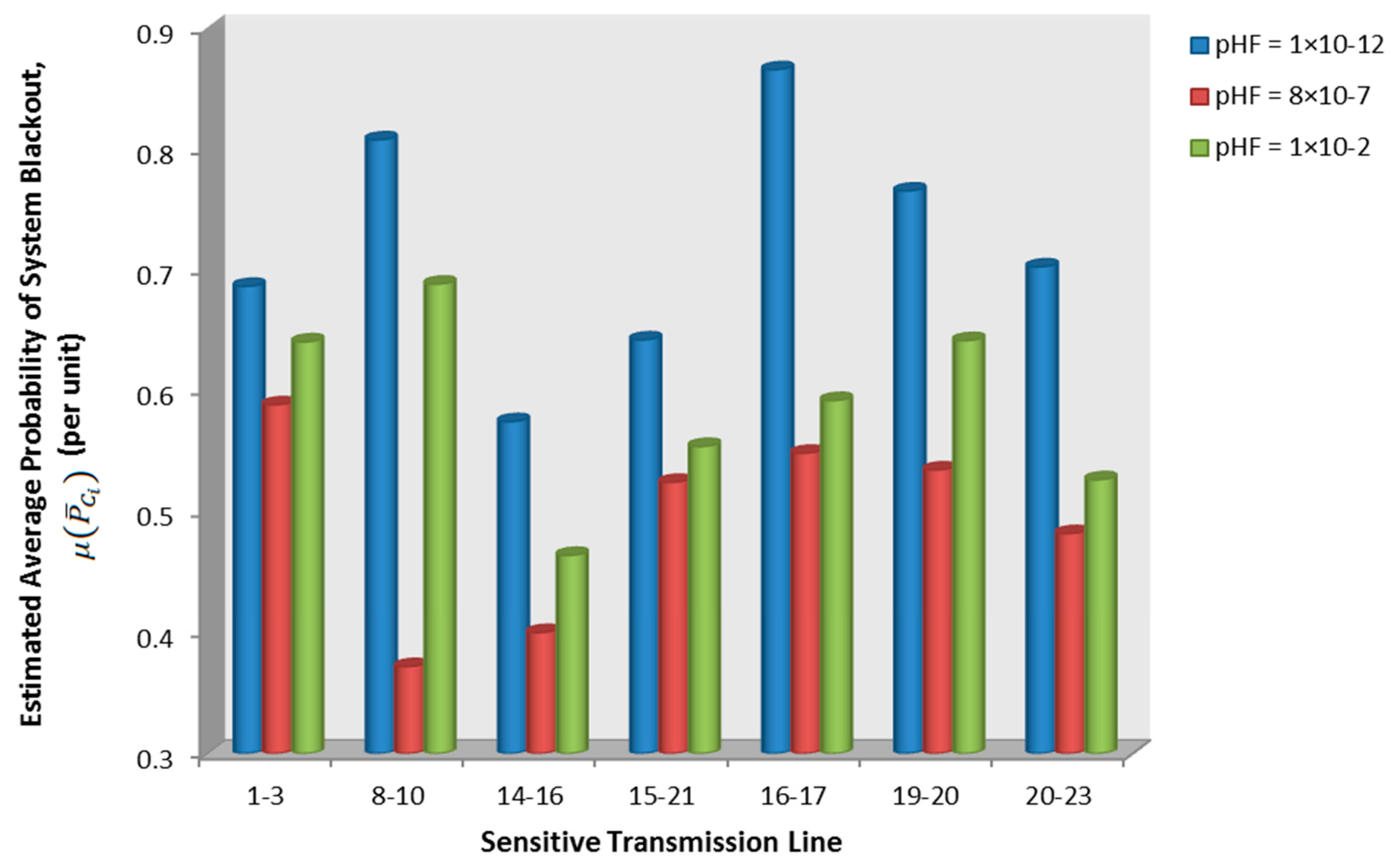
Figure 5 shows the results of for each initial sensitive transmission line tripping at three different cases of relay hidden failure for IEEE RTS-79. However, the results shown in Figure 5 only depict selected sensitive initial transmission line tripping that have large values of . For all three case studies, the is arranged to specify the sensitive transmission lines that have a significant contribution to a critical dynamic power system blackout. The discussion emphasizes the relatively large value of that signifies the chosen initial transmission line tripping is sensitive to the dynamic system operating condition causing to the occurrence of critical dynamic power system blackout. In the figure, it is observed that the value of for the case of pHF = 1 × 10⁻¹² is higher than the cases where pHF = 8 × 10⁻⁷ and pHF = 1 × 10⁻². It is noted in Section 2.3 that the historical information of power system blackout provides the inherent pHF value of 8 × 10⁻⁷, which has the lowest value for the majority of sensitive initial transmission lines tripping. This result implies that accurate estimation of hidden failure probability has a significant impact on the result of risk assessment in dynamic power system blackout.
Figure 6 presents the tabulation of selected sensitive transmission lines arranged according to the risk assessment of dynamic power system blackout, . According to [32], IEEE RTS-96 comprises 120 transmission lines. Nevertheless, similar to the aforementioned analysis, the selected results of sensitive initial transmission lines refer to the largest risks of dynamic power system blackout, . Similar to the above analysis, the risk based of dynamic power system blackout for IEEE RTS-96 is analyzed under three types of relay hidden failure. The findings are similar to the analysis shown above in Figure 5, where there is significant difference of risk based between each initial tripping of sensitive transmission line. However, the case of pHF = 1 × 10⁻² causes all sensitive transmission lines to acquire that is higher than the of pHF = 8 × 10⁻⁷ and pHF = 1 × 10⁻¹². Nevertheless, the exact value for the case of pHF = 8 × 10⁻⁷ brings the same conclusion: the can be regarded as low for IEEE RTS-96, as depicted in Figure 6, which is similar to the IEEE RTS-79 (Figure 5). This signifies that determination of the exact value of hidden failure probability plays an important role, since it will render the right conjecture with an accurate result in the risk assessment of dynamic power system blackout.
3.2. Comparison of Sensitive Transmission Lines Tripping Associated with the Static and Dynamic Power System Blackouts
This section will discuss the comparison of the sensitive initial transmission lines tripping corresponding to the risk based of static [29,33] and dynamic power system blackouts. IEEE RTS-79 and IEEE RTS-96 are used as the case studies for comparison of the sensitive transmission lines tripping, as depicted in Figure 7 and Figure 8, respectively.
Figure 7 represent the comparison of sensitive initial transmission lines tripping with respect to the risk assessment of static and dynamic power system blackouts for the case study of IEEE RTS-79. In relation to the static power system blackout, pHF = 8 × 10⁻⁷ causes the sensitive initial transmission line tripping to have a that is higher than the pHF = 1 × 10⁻¹² and pHF = 1 × 10⁻² cases. The pHF = 1 × 10⁻² case confers the lowest value, for almost all of the sensitive initial transmission lines tripping related to the case of static power system blackout. Contradictorily, with , in the case of dynamic power system blackout , pHF = 1 × 10⁻¹² causes all of the sensitive initial transmission lines tripping to obtain a that is higher than the of the pHF = 8 × 10⁻⁷ and pHF = 1 × 10⁻² cases. The pHF = 8 × 10⁻⁷ case exerts to the lowest for all of the initial sensitive line tripping for the case of dynamic power system blackout. Cmparative studies show that the pHF = 8 × 10⁻⁷ case causes the highest value for all initial sensitive lines tripping under the static power system blackout case study. The results contradict the outcomes acquired from the dynamic power system blackout case studies in that the highest value for all of the initial sensitive transmission lines tripping are attained subject to the pHF = 1 × 10⁻¹² case. Therefore, for the case study of static power system blackout, pHF = 1 × 10⁻² causes the lowest value for all of the initial sensitive transmission lines tripping. This contrasts with the dynamic power system blackout case study in which the lowest is imposed by pHF = 8 × 10⁻⁷. These results highlight that the dynamic power system blackout has a tangible impac,t causing a large value of for all of the initial sensitive transmission lines tripping as compared to the impact of static power system blackout. The results also imply that uncertain tripping of the exposed generator as well as the exposed transmission line may cause a worse condition due to considerable risk in the power system operation originated from the dynamic power system blackout.
Comparison of the values obtained based on the case of static and dynamic power system blackout is also performed on the IEEE RTS-96 test system, as shown in Figure 8. Similar to the above-mentioned discussion for the case study of IEEE RTS-79, in relation to the occurrence of static power system blackout, it is obvious that pHF = 8 × 10⁻⁷ and pHF = 1 × 10⁻¹² give similar results for . In addition, the results also have shown that the pHF = 1 × 10⁻² case causes the sensitive initial transmission line tripping to have a that is lower than the pHF = 1 × 10⁻¹² and pHF = 8 × 10⁻⁷ cases. On the other hand, the pHF = 1 × 10⁻¹² case exerts the highest for all of the sensitive initial transmission lines tripping, subject to the occurrence of static power system blackout. Under the perspective of dynamic power system blackout, pHF = 1 × 10⁻² causes the highest value of for most of the initial sensitive line trippings compared to the pHF = 1 × 10⁻¹² and pHF = 8 × 10⁻⁷ cases. Contradictory to the results of that can be observed for the case of dynamic power system blackout, the pHF = 8 × 10⁻⁷ case causes most of the sensitive transmission lines to obtain a that is lower than the of pHF = 1 × 10⁻¹² and pHF = 1 × 10⁻² cases. From the results shown in Figure 8, a large value of , for all of the initial transmission lines tripping that cause a worse power system operating condition, is attained, corresponding to the dynamic power system blackout in contrast with the impact of static power system blackout.
The occurrence of dynamic power system blackout may cause a worse power system operating condition because of a that is larger, as compared to the results obtained based on the static power system blackout. Despite this, it is important to perform a dynamic power system blackout, which has a significant impact on the risk assessment of a power system operation.
Albeit, for both case studies, the risk of dynamic power system blackout is greater than the risk of static power system blackout, as depicted in Figure 7 and Figure 8. However, a significant difference in terms of its range in the risk of static power system blackout can be observed by comparing the results obtained from IEEE-RTS79 and IEEE-RTS69 given in Figure 7 and Figure 8, respectively. It can be assumed that this problem stems from the transmission line outage solely considered as the tripping parameter performed in the procedure of static power system blackout. This may cause a lower and inconsistent range in the risk of static power system blackout, which can be observed via the comparison of results obtained from the IEEE RTS-79 and IEEERTS-96. Therefore, it is imperative to take into account the critical parameters of transmission line, generator rotor angle and frequency generator, which will significantly affect the power system operating condition, to provide more accurate results with higher and consistent range for the risk of dynamic power system blackout system observed through the comparison between the IEEE RTS-79 and IEEE RTS-96.
3.3. Determination of Severe Total Loading Condition Based on the Risk of Dynamic Power System Blackout
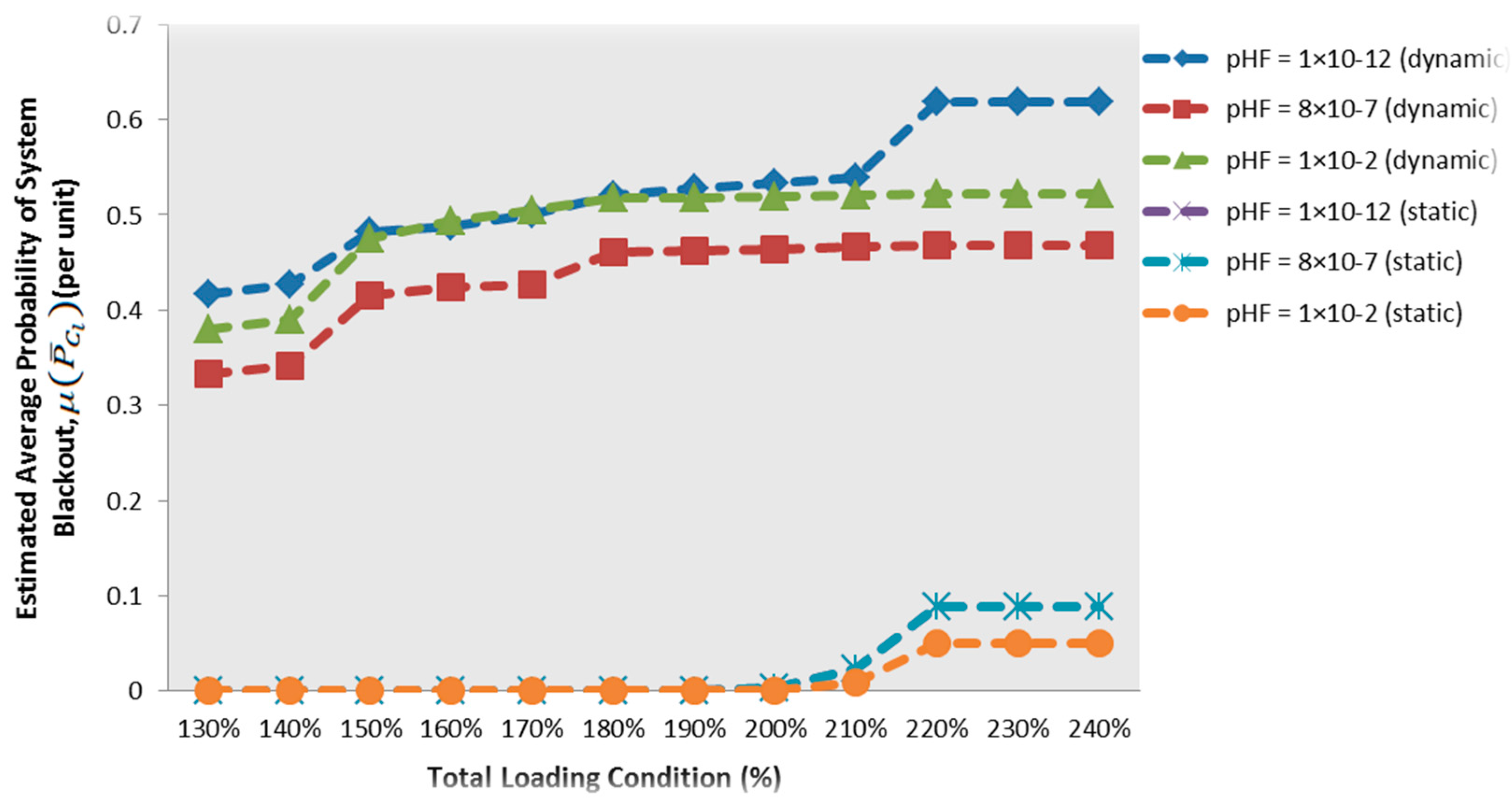
The determination of severe total loading condition is performed by referring to the risk based of critical dynamic power system blackout. It is worth noting that the three case studies originate from [29], and are further explored for in-depth analysis of the proposed approach that will be discussed in this section. Figure 9 shows the results of representing the risk of dynamic power system blackout attributed to a 150–240% increased of total loading condition taking into account three different types of pHF. The beginning of system operating risk for the IEEE RTS-79 arises during 150% increase of total loading condition. The severity of dynamic power system blackout starts to appear at 160% increase of total loading condition. The results are obtained based on the three cases of pHF = 8 × 10⁻⁷, pHF = 1 × 10⁻¹² and pHF = 1 × 10⁻². A significant increase of can be seen for all the three case studies, when there is beyond 160% increased of total loading condition. From the three different case studies, pHF = 1 × 10⁻² is causing to the most critical condition in the risk assessment compared to the obtained based on pHF = 1 × 10⁻¹² and pHF = 8 × 10⁻⁷ cases.
The results have shown that determination of an accurate pHF value is important, notably when there is a severe increase of total loading condition causing to a significant impact on the emergence of critical dynamic power system blackout. The historical information of power system blackout provides the inherent pHF value of 8 × 10⁻⁷, which has the lowest value at every total loading condition. The results signify the importance of determining the risk of dynamic power system blackout that takes into account the accurate estimation of hidden failure probability values considering the historical information of power system blackouts.
The above-mentioned discussion is similar to the result of risk based in determining the critical dynamic power system blackout for the IEEE RTS-96. Figure 10 shows a rapid increase for the results of risk based with the 130–220% increase of total loading condition. In the case study of IEEE RTS-96, the risk of system operating condition starts to emerge when the total system loading condition is increased by 130%. By referring to the three types of pHF, the system begins to experience a critical dynamic power system blackout as the total loading condition is severely increased above 140%. It is noticeable that the value of starts to increase in conjunction with a 140% of total loading condition. This refers to pHF = 1 × 10⁻¹² inflicting the largest amount of in contrast with the risk acquired via the pHF = 8 × 10⁻⁷ and pHF = 1 × 10⁻². Albeit the lowest value incurred for all of the increased total loading conditions with pHF = 8 × 10⁻⁷, it is still important to record the historical information of power system blackout so that the hidden failure probability of pHF = 8 × 10⁻⁷ is accurately determined, which is indispensible for the risk assessment of dynamic power system blackout.
The results related to the for the case study of RTS-79 and IEEE RTS-96 implies that inaccurate value of pHF will adversely affect the result of critical dynamic power system blackout adversely afflicted by the severe total loading condition. The inherent value of pHF = 8 × 10⁻⁷ obtained from the historical information of power system blackout results in the lowest risk based of dynamic power system blackout for both test systems. Therefore, it is important for the power marketers and utilities to identify the correct value of pHF, which significantly impacts the severely increased total loading condition against the emergence of critical dynamic power system blackout. Besides that, marketers and utilities will encounter ineffective electricity trading as this consequence is caused by inaccurate estimation of dynamic power system blackout disrupted by the discrepancies of pHF value.
3.4. Comparison of Severe Total Loading Condition under the Perspective of Static and Dynamic Power System Blackouts
This section explains the comparative results of severe total loading condition obtained corresponding to the static [29,33] and dynamic power system blackouts for IEEE RTS-79 and IEEE RTS-96. Figure 11 depicts the results of which represents the severity of total loading condition for static and dynamic power system blackouts with regard to the implication of protection system hidden failure for the case study of IEEE RTS-79.
In conjunction with the case study of static power system blackout, it is observed that pHF = 8 × 10⁻⁷ and pHF = 1 × 10⁻² produce similar high values of risk based for most increments of the total loading conditions, followed by pHF = 1 × 10⁻¹². Contradictory to the results of adversely implicated by the dynamic power system blackout, pHF = 8 × 10⁻⁷ produces the lowest risk based for every increment of total loading condition in comparison to pHF = 1 × 10⁻² and pHF = 1 × 10⁻¹². The comparative studies emphasize that pHF = 8 × 10⁻⁷ causes the largest value corresponding to the case study of static power system blackout. This conflicts with the results obtained based on the case study of dynamic power system blackout that pHF = 8 × 10⁻⁷ causes the lowest value of . For all the three cases of pHF, it is obvious that the of total loading condition is rather small for the static power system blackout. On the other hand, the total loading condition and dynamic power system blackout severely cause relatively large value of in the power system operation. Therefore, it is worth noting that uncertainty in the exposed generator and exposed transmission line tripping, compounded with the rapid increased of total loading condition above 140%, will severely aggravate the implication of dynamic power system blackout.
With regards to the case study of IEEE RTS-96, comparative study based on the results of is performed to distinguish significant deterioration in the power system operation originated either from the static or dynamic power system blackouts afflicted by the hidden failure compounded with the severe total loading condition, as shown in Figure 12. By referring to the results of obtained in accordance with the static power system blackout, pHF = 1 × 10⁻¹² and pHF = 8 × 10⁻⁷ produce similar results for , which are higher than the value of for pHF = 1 × 10⁻². On the other hand, for the dynamic power system blackout, pHF = 8 × 10⁻⁷ produces the lowest risk based for every increment of total loading condition followed by pHF = 1 × 10⁻¹² and pHF = 1 × 10⁻².
In the case study of IEEE RTS-96, the results divulge the largest value incurred by pHF = 8 × 10⁻⁷ during the case study of static power system blackout. Conversely, in the case of dynamic power system blackout, pHF = 8 × 10⁻⁷ causes the lowest for every total loading condition increment. For all three cases of pHF, it is obvious that the of total loading condition is rather small for the static power system blackout. However, the dynamic power system blackout produces relatively large value of for the total loading condition. Therefore, this implies that a severe power system operating condition is exacerbated due to the occurrence of dynamic power system blackout emanating from the uncertainty of exposed generator and exposed transmission lines tripping, compounded by the rapid increase of total loading condition above 130%. Similar to the findings discussed above in relation to Figure 11, the results shown in Figure 12 attest that the dynamic power system blackout undertaken according to the three case studies of pHF yield a considerably large value of compared to the results obtained based on the static power system blackout. This is because the overloaded transmission line, dynamic violation of generator rotor angle limit and dynamic violation of generator frequency limit are additional limitations of power system parameters considered in the procedure of the dynamic power system blackout that is discussed in Section 2.3.
4. Conclusions
This study developed a new framework of stochastic event tree used for sustainability assessment in a power system operation pertaining to the impact of dynamic power system blackout. In depth analysis has been carried out based on two types of risk assessment in power system operating condition, static and dynamic power system blackouts, customarily caused by disoperation or hidden failure of a protection system. The obtained results imply that it is important to determine a realistic value in the probability of hidden value, which is pHF = 8 × 10⁻⁷, as it gives a higher risk of dynamic power system blackout. Comparative studies conducted between two types of risk assessment in system operating conditions signify that the dynamic power system blackout confers a higher risk in contrast to the static power system blackout. This is because the dynamic power system blackout was designed by means of propagation in the exposed power system component tripping attributed by the overloaded transmission line, violation of generator rotor angle limit or intrusion of generator frequency limit. This contradicts the insignificant result of static power system blackout that solely takes into account the propagation tripping of overloaded transmission line as the violation of steady state system operating constraint. In addition, by utilizing the proposed stochastic event tree technique for risk assessment of dynamic power system blackout, it is beneficial and useful to utility and power system planners because of its robustness to identify the sensitive transmission lines and severity of total loading conditions that have the potential to cause critical dynamic power system blackouts. Eventually, pragmatic implementation of the proposed concept will assist utility and power system planners to stipulate the best action to avert problems related to the sustainable power system operating condition.
Acknowledgments
This research project is undertaken under the auspices of research grants FRGS/2/2014/TK03/UITM/02/1, RAGS/1/2014/TK03/UITM//6, 600-RMI/DANA 5/3/LESTARI (77/2015) and 600-IRMI/DANA/5/3/BESTARI(0001/2016) conferred by the Ministry of Higher Education (MOHE), Malaysia and the Institute of Research Management & Innovation (IRMI), Universiti Teknologi MARA, Malaysia.
Author Contributions
All of the authors have participated in the preparation of the manuscript. Muhammad Murtadha Othman and Ismail Musirin participated in initial discussion for deciding the methodology used for solving the problems. Muhammad Murtadha Othman and Nur Ashida Salim devised the experiments. Nur Ashida Salim performed all the simulation work, gathered important results and drafted the article. Ismail Musirn helpd interpret the data and results. The main revisions were done by all of the authors before finalizing the manuscript.
Conflicts of Interest
The authors declare no conflict of interest.
References
- Aghamohammadi, M.R.; Hashemi, S.; Hasanzadeh, A. A new approach for mitigating blackout risk by blocking minimum critical distance relays. Int. J. Electr. Power Energy Syst. 2016, 75, 162–172. [Google Scholar] [CrossRef]
- Belkacemi, R.; Bababola, A.; Zarrabian, S.; Craven, R. Multi-agent system algorithm for preventing cascading failures in smart grid systems. In Proceedings of the North American Power Symposium (NAPS), Pullman, WA, USA, 7–9 September 2014. [Google Scholar]
- Li, Y.F.; Sansavini, G.; Zio, E. Non-dominated sorting binary differential evolution for the multi-objective optimization of cascading failures protection in complex networks reliability. Eng. Syst. Saf. 2013, 111, 195–205. [Google Scholar] [CrossRef]
- Scala, A.; Lucentini, P.G.D.S.; Caldarelli, G.; D’Agostino, G. Cascades in interdependent flow networks. Phys. D Nonlinear Phenom. 2016, 323, 35–39. [Google Scholar] [CrossRef]
- Scala, A.; Lucentini, P.G.D.S. The equal load-sharing model of cascade failures in power grids. Phys. A Stat. Mech. Appl. 2016, 462, 737–742. [Google Scholar] [CrossRef]
- Ke, S.; Zhen-Xiang, H. Analysis and comparison on several kinds of models of cascading failure in power system. In Proceedings of the 2005 IEEE/PES Transmission and Distribution Conference and Exhibition: Asia and Pacific, Dalian, China, 18 August 2005. [Google Scholar]
- Zhou, B.; Li, R.; Cheng, L. A risk assessment model of power system cascading failure considering the impact of ambient temperature. In Proceedings of the 2014 Asia-Pacific Conference on Electronics and Electrical Engineering, Shanghai, China, 27–28 December 2015. [Google Scholar]
- Henneaux, P.; Song, J.; Cotilla-Sanchez, E. Dynamic probabilistic risk assessment of cascading outages. In Proceedings of the 2015 IEEE Power & Energy Society General Meeting, Denver, CO, USA, 26–30 July 2015. [Google Scholar]
- Henneaux, P.; Labeau, P.E.; Maun, J.C.; Haarla, L. A two-level probabilistic risk assessment of cascading outages. IEEE Trans. Power Syst. 2016, 31, 2393–2403. [Google Scholar] [CrossRef]
- Henneaux, P.; Labeau, P.E.; Maun, J.C. A level-1 probabilistic risk assessment to blackout hazard in transmission power systems. Reliab. Eng. Syst. Saf. 2012, 102, 41–52. [Google Scholar] [CrossRef]
- Xue, Y.; Van Custem, T.; Ribbens-Pavella, M. Extended equal area criterion justifications, generalizations, applications. IEEE Trans. Power Syst. 1989, 4, 44–52. [Google Scholar] [CrossRef]
- Xue, Y.; Van Cutsem, T.; Ribbens-Pavella, M. A simple direct method for fast transient stability assessment of large power systems. IEEE Trans. Power Syst. 1998, 3, 400–412. [Google Scholar] [CrossRef]
- Bhat, S.; Glavic, M.; Pavella, M.; Bhatti, T.S.; Kothari, D.P. A transient stability tool combining the SIME method with MATLAB and SIMULINK. Int. J. Electr. Eng. Educ. 2006, 43, 119–133. [Google Scholar] [CrossRef]
- Pizano-Martínez, A.; Fuerte-Esquivel, C.R.; Zamora-Cárdenas, E.; Ruiz-Vega, D. Selective transient stability-constrained optimal power flow using a SIME and trajectory sensitivity unified analysis. Electr. Power Syst. Res. 2014, 109, 32–44. [Google Scholar] [CrossRef]
- Busan, S. Dynamic Available Transfer Capability Calculation Considering Generation Rescheduling. Master’ Thesis, Universiti Teknologi MARA, Shah Alam, Malaysia, September 2012. [Google Scholar]
- Busan, S.; Othman, M.M.; Musirin, I.; Mohamed, A.; Hussain, A. A new algorithm for the available transfer capability determination. Math. Probl. Eng. 2010, 2010, 795376. [Google Scholar] [CrossRef]
- Li, Y.H.; Yuan, W.P.; Chan, K.W.; Liu, M.B. Coordinated preventive control of transient stability with multi-contingency in power systems using trajectory sensitivities. Int. J. Electr. Power Energy Syst. 2011, 33, 147–153. [Google Scholar] [CrossRef]
- Yuan, Y.; Kubokawa, J.; Sasaki, H. A solution of optimal power flow with multicontingency transient stability constraints. IEEE Trans. Power Syst. 2003, 18, 1094–1102. [Google Scholar] [CrossRef]
- Xia, Y.; Chan, K.W. Dynamic constrained optimal power flow using semi-infinite programming. IEEE Trans. Power Syst. 2006, 21, 1455–1457. [Google Scholar] [CrossRef]
- Pizano-Martianez, A.; Fuerte-Esquivel, C.R.; Ruiz-Vega, D. Global transient stability-constrained optimal power flow using an OMIB reference trajectory. IEEE Trans. Power Syst. 2010, 25, 392–403. [Google Scholar] [CrossRef]
- Duong, M.Q.; Grimaccia, F.; Leva, S.; Mussetta, M.; Le, K.H. Improving transient stability in a grid-connected squirrel-cage induction generator wind turbine system using a fuzzy logic controller. Energies 2015, 8, 6328–6349. [Google Scholar] [CrossRef]
- Duong, M.Q.; Sava, G.N.; Grimaccia, F.; Leva, S.; Mussetta, M.; Costinas, S.; Golovanov, N. Improved LVRT based on coordination control of active crowbar and reactive power for doubly fed induction generators. In Proceedings of the 2015 9th International Symposium on Advanced Topics in Electrical Engineering (ATEE), Bucharest, Romania, 7–9 May 2015. [Google Scholar]
- Takada, H.; Kato, Y.; Iwamoto, S. Transient stability preventive control using CCT and generation margin. In Proceedings of the Power Engineering Society Summer Meeting, Vancouver, BC, Canada, 15–19 July 2001. [Google Scholar]
- Kato, Y.; Iwamoto, S. Transient stability preventive control for stable operating condition with desired CCT. IEEE Trans. Power Syst. 2002, 17, 1154–1161. [Google Scholar] [CrossRef]
- Fujii, W.; Wakisaka, J.; Iwamoto, S. Transient stability analysis based on dynamic single machine equivalent. In Proceedings of the 39th North American Power Symposium, Las Cruces, NM, USA, 30 September–2 October 2007. [Google Scholar]
- Bae, K.; Thorp, J.S. A stochastic study of hidden failures in power system protection. Decis. Support Syst. 1999, 24, 259–268. [Google Scholar] [CrossRef]
- Chen, J.; Thorp, J.S.; Dobson, I. Cascading dynamics and mitigation assessment in power system disturbances via a hidden failure model. Int. J. Electr. Power Energy Syst. 2005, 27, 318–326. [Google Scholar] [CrossRef]
- Yang, F.; Meliopoulos, A.S.; Cokkinides, G.J.; Dam, Q.B. Effects of protection system hidden failures on bulk power system reliability. In Proceedings of the 38th North American Power Symposium, 2006 (NAPS 2006), Carbondale, IL, USA, 17–19 September 2006. [Google Scholar]
- Salim, N.A.; Othman, M.M.; Musirin, I.; Serwan, M.S. Determination of sensitive transmission lines due to the effect of protection system hidden failure in a critical system cascading collapse. Int. J. Electr. Comput. Energ. Electron. Commun. Eng. 2013, 7, 548–553. [Google Scholar]
- Chen, G.; Dong, Z.Y.; Hill, D.J.; Zhang, G.H.; Hua, K.Q. Attack structural vulnerability of power grids: A hybrid approach based on complex networks. Phys. A Stat. Mech. Appl. 2010, 389, 595–603. [Google Scholar] [CrossRef]
- Probability Methods Subcommittee. IEEE reliability test system. IEEE Trans. Power Appar. Syst. 1979, PAS-98, 2047–2054. [Google Scholar]
- Grigg, C.; Wong, P.; Albrecht, P.; Allan, R.; Bhavaraju, M.; Billinton, R.; Chen, Q.; Fong, C.; Haddad, S.; Kuruganty, S.; et al. The IEEE reliability test system-1996. A report prepared by the Reliability Test System Task Force of the Application of Probability Methods Subcommittee. IEEE Trans. Power Syst. 1999, 14, 1010–1020. [Google Scholar]
- Dobson, I.; Newman, D.E. Cascading blackout overall structure and some implications for sampling and mitigation. Int. J. Electr. Power Energy Syst. 2017, 86, 29–32. [Google Scholar] [CrossRef]
Figure 1.
A single line diagram of the IEEE RTS-79 system.

Figure 2.
A single line diagram of the IEEE RTS-96 system.

Figure 3.
Transient response of subsequent to the initial tripping of line 1–3: (a) CCT specified based on the lowest of 0.01 s; and (b) CCT specified based on the of 0.02 s.
Figure 3.
Transient response of subsequent to the initial tripping of line 1–3: (a) CCT specified based on the lowest of 0.01 s; and (b) CCT specified based on the of 0.02 s.

Figure 4.
Transient response of subsequent to the initial tripping of line 101–103: (a) CCT specified based on the lowest of 0.01 s; and (b) CCT specified based on the of 0.02 s.
Figure 4.
Transient response of subsequent to the initial tripping of line 101–103: (a) CCT specified based on the lowest of 0.01 s; and (b) CCT specified based on the of 0.02 s.

Figure 5.
Sensitive initial transmission line tripping obtained based on the for the IEEE RTS-79.

Figure 6.
Sensitive initial transmission line tripping obtained based on the for the IEEE RTS-96.

Figure 7.
Comparison of risk based under the case study of IEEE RTS-79.

Figure 8.
Comparison of risk based for the case study of IEEE RTS-96.

Figure 9.
The implication of total loading condition increment towards the risk based for the case study of dynamic power system blackout in an IEEE RTS-79.
Figure 9.
The implication of total loading condition increment towards the risk based for the case study of dynamic power system blackout in an IEEE RTS-79.

Figure 10.
Implication of total loading condition into against the risk based for the case study of dynamic power system blackout in an IEEE RTS-96.
Figure 10.
Implication of total loading condition into against the risk based for the case study of dynamic power system blackout in an IEEE RTS-96.

Figure 11.
Significance of static and dynamic power system blackout to the risk based for the case study of for IEEE RTS-79.
Figure 11.
Significance of static and dynamic power system blackout to the risk based for the case study of for IEEE RTS-79.

Figure 12.
Significance of static and dynamic power system blackout to the risk based for the case study of IEEE RTS-96.
Figure 12.
Significance of static and dynamic power system blackout to the risk based for the case study of IEEE RTS-96.

© 2017 by the authors. Licensee MDPI, Basel, Switzerland. This article is an open access article distributed under the terms and conditions of the Creative Commons Attribution (CC BY) license (http://creativecommons.org/licenses/by/4.0/).
Share and Cite
MDPI and ACS Style
Othman, M.M.; Salim, N.A.; Musirin, I. Sustainability from the Occurrence of Critical Dynamic Power System Blackout Determined by Using the Stochastic Event Tree Technique. Sustainability 2017, 9, 941. https://doi.org/10.3390/su9060941
AMA Style
Othman MM, Salim NA, Musirin I. Sustainability from the Occurrence of Critical Dynamic Power System Blackout Determined by Using the Stochastic Event Tree Technique. Sustainability. 2017; 9(6):941. https://doi.org/10.3390/su9060941
Chicago/Turabian StyleOthman, Muhammad Murtadha, Nur Ashida Salim, and Ismail Musirin. 2017. "Sustainability from the Occurrence of Critical Dynamic Power System Blackout Determined by Using the Stochastic Event Tree Technique" Sustainability 9, no. 6: 941. https://doi.org/10.3390/su9060941
Note that from the first issue of 2016, this journal uses article numbers instead of page numbers. See further details here.