
Land Cover Changes (1963–2010) and Their Environmental Factors in the Upper Danube Floodplain


1
Division of Landscape Ecology and Landscape Planning, Institute of Landscape Ecology and Resources Management, Justus-Liebig-University Giessen, 35392 Giessen, Germany
2
Department of Landscape Ecology, Institute for Natural Resource Conservation, Christian-Albrechts-University of Kiel, 24098 Kiel, Germany
*
Author to whom correspondence should be addressed.
Sustainability 2017, 9(6), 943; https://doi.org/10.3390/su9060943
Submission received: 4 May 2017
/
Revised: 24 May 2017
/
Accepted: 31 May 2017
/
Published: 3 June 2017
(This article belongs to the Section Environmental Sustainability and Applications)
Abstract
:To analyze the changes in the Upper Danube Floodplain, we used aerial photos to quantify the change of landscape pattern from 1963 to 2010. We focused on typical floodplain habitats, i.e., riparian forest and floodplain grassland. We used landscape metrics and transformation matrix to explore changes in land cover structure and composition. The active floodplain experienced increasing fragmentation from 1963 to 2010. Despite an increase of aggregation, riparian forest suffered a 2.3% area loss from 1995 to 2010. Arable land in the active floodplain declined by 28.5%, while its patch size significantly increased. Elevation, distance to river and soil quality were the most relevant environmental factors for the land cover change in the floodplain. Higher soil quality or longer distance to river led to an increase of conversion from grassland into arable land; grassland patches with poorer soil quality were likely to change into riparian forest; riparian forest closer to the river and with a lower height above mean water level tended to remain stable. This comprehensive understanding of historical land cover change and environmental factors is needed for the enhancement of landscape functions and sustainable development in the floodplain.
1. Introduction
Natural and semi-natural floodplain habitats are valuable but rare. As an essential component of riverine ecosystems, riparian forests would form the Potential Natural Vegetation (PNV) that would theoretically develop without human influence [1,2]. Riparian forests have a high biomass productivity and habitat value. They provide various functions including water storage, water quality improvement, protection against flood and erosion, dead-wood provision for the structural diversity of the river, and they act as a buffer against negative influences of adjacent agricultural and industrial activities [3]. In many European floodplains, riparian forests were reduced or disappeared because of the river management activities. Consequently, riparian forests became threatened floodplain habitats [4].
Floodplain grasslands harbor exceptionally high numbers of species [5]. They experience periodic flooding and they are regularly mown or grazed. Grasslands in floodplains without nature protection measures have experienced alarming losses since the 1950s [6]. This loss is attributed to land drainage, fertilizer uses and the conversion from grassland to cropland [7].
The riparian landscape has changed tremendously over time in various floodplains worldwide [8]. In Europe, the Danube is an example for this: since the beginning of the 19th century, 80% of the Danube Floodplain has been lost due to river regulation, land cover change and dam construction [9]. Compared with other stretches, especially the Upper Danube River has suffered significant modification in the last two centuries [10]. The anthropogenic influence on the Danube River can be clustered into several phases [11]: from the 18th century to the 1850s, meanders were cut off and the riverbed was narrowed to raise the transportation capacity; from the 1850s to 1900, low water regulations for waterway transport and sediment extractions for construction uses were implemented. Land parceling and settlement growth in the 19th century continuously changed the Danube Floodplain [12]. At the beginning of the 20th century, power plants were constructed and more dredging projects followed. Many gravel pits were built along the river from 1950 to 1960 [13]. Flood control, navigation, and hydroelectric power plants caused many problems: alteration of the riverine landscape, degradation of the river bed, decoupling of the floodplain from the river, disturbance of the lateral connectivity and exchange processes, restriction of hydro-morphological dynamics, reduction of habitat variability and biodiversity [14]. Dam construction and river regulation may prevent flooding, cause sediment deficit and change hydro-geomorphic patterns, which further disrupt the composition and structure of riparian vegetation [15,16]. In case of the Danube Floodplain, changes of the ground-water level led to the degradation of forest and other riparian vegetation types [17].
Land cover in the past can control or constrain current land cover composition, and changing trends may affect ecosystem development in the future [18]. Previous researchers have demonstrated the influences of historical land cover structure on the current diversity of plant species [19]. Habitat loss and other environmental changes can cause delayed responses of some species, which is called the extinction debt [20]. The conditions are no longer suitable for the persistence of some plant species, and they will go extinct in the future [19]. However, provided the species persist, there is time to implement habitat restoration and other measures [21]. A clear understanding of land cover change reveals the threats to biodiversity and helps to establish better conservation measures.
From the middle of the last century, the conversion from riparian forest to agricultural land and urban area occurred in Central Europe (e.g., the Middle Elbe River [22]) and worldwide (e.g., the Upper Mississippi River [23], the Laoha River [24], the Willamette Valley [25]). Other riparian land cover types (e.g., grassland, fallow land) were converted to arable and urban land [24]. Conversely, the conversion from other land over (e.g., open land) to woodland led to an expansion of riparian forest in some European floodplains (e.g., the Magra River [26], the Lech River [27]) and worldwide (e.g., the Upper San Pedro River [28]). However, some studies found no fundamental changes in the forest cover, but rather the conversion of agricultural land from extensive permanent grassland to intensive arable land [29]. As a general trend, human influence in most of the floodplains is increasing, which is in conflict with nature conservation [30]. This trend calls for alerts and threatens the need for more natural floodplain landscapes.
The fundamental method to quantify the temporal evolution of land cover is to interpret satellite images/aerial photos [16,26,31]. Landscape metrics, based on the geometry (e.g., number, size, shape and distribution) of patches of different land cover types, have been used to quantify landscape change [32,33]. Researchers selected metrics based on specific categories (e.g., shape, fragmentation, and diversity) [34,35]: Lausch and Herzog [36] selected a few metrics (e.g., MPS (mean patch size) and IJI (interspersion and juxtaposition index)) from various metrics to monitor the landscape structure in Leipzig South region and Espenhaim; Zhao et al. [37] applied fragmentation metrics (e.g., MPS or LPS (largest patch index)), shape metrics (e.g., LSI (landscape shape index)) and diversity metrics (e.g., SHDI (Shannon’s diversity index), SHEI (Shannon’s evenness index)) to assess the impact of dam construction on the change of landscape patterns in the Lancang River Basin.
Several studies analyzed the influence of environmental factors on the riparian landscape. Topographic variables (e.g., elevation, slope, aspect etc.) were estimated to affect the land cover changes [38]. Climatic gradients, inundation, soil moisture, nutrients and disturbance affect the riparian vegetation [30,39,40]. Within the catchment, elevation and distance from the river in general have the primary influence on the composition and structure of riparian vegetation [41]. Along the lateral gradient, elevation increases from the river channel to the upland and reflects the topographic features in the floodplain (e.g., levees) [41]. However, some studies found the modern forest distribution is decoupled from the natural environmental conditions [42]. In the floodplain landscape with agriculture as the major component, the arable land tends to occur in the coarse-grained natural levee/point bar close to the river channel, where it is infrequently flooded with rapid drainage; however, the pasture land was more associated with the cohesive clayey deposits such as the backswamp, where it is seasonally flooded with poor drainage [31]. Due to the dynamic characteristics of the floodplain, the mechanism of the relationship between environmental factors and the change of floodplain habitats is complicated. Not only the river stage, but also the spatial variability of floodplain geomorphology in the large river system affects the floodplain water table [43].
Although many studies have been conducted about the long-term land cover change in the floodplain, most of them were done at a coarse scale (e.g., 1 km2) or they were conducted as case studies [29,44]. For example, Jones et al. [45] studied riparian land cover change (1972–2003) across the continental United States at the catchment and riparian scales and they found the decline of natural land cover (e.g., forest) as well as the increase of agricultural and urban land. Since floodplain biotopes are rather small and dynamic, studies at a finer scale are needed to enable a more detailed and accurate understanding of land cover change in the floodplain. To fill this knowledge gap, we used the land cover analysis scale of 1:5000 in our study, which enables a more detailed and accurate understanding of how the land cover in the floodplain changed at the finer scale. The larger number of study sites makes the comparison possible.
The objectives of this study were (1) to determine past land cover pattern of floodplain with regard to the importance for ecological structures and functions; (2) to identify the relationship between environmental factors and land cover change; (3) to assess the observed trends in a floodplain context for a more sustainable floodplain development. We focused on the changes of riparian forest and floodplain grassland owing to their unique importance to the floodplain. Besides a clear understanding of land cover change and the environmental factors, land cover change should be evaluated from an ecological point of view. The following research questions were addressed:
- How did the land cover pattern, i.e., the land cover composition and structure, change from 1963 to 2010 in the Upper Danube Floodplain?
- ○
- How did the grassland pattern change?
- ○
- How did the riparian forest pattern change?
- Which environmental factors are related to land cover change (especially grassland and riparian forest changes) in the active Upper Danube Floodplain?
- Which are the ecological consequences of the recorded trends in a floodplain context?
To conduct a comprehensive and comparable study about the long-term changes in a floodplain, we analyzed the land cover change in the Upper Danube Floodplain in a 50-year time span. We chose this study period (1963–2010) because in the 1950s German agriculture prospered due to a large demand for food after World War II [46]. Since the 1960s, the German agricultural policy has been regulated at a European level. This greatly altered agricultural production methods in Germany, which influenced the land cover change nationwide [47].
2. Materials and Methods
2.1. Study Area
The study area is located along the Upper Danube River in Bavaria, Southern Germany (River-km 2,379–2,245) (Figure 1). The Danube River is an important international waterway, which origins from the Black Forest, passes through ten countries and finally enters the Black Sea; it has a pluvial-nival flow regime. As an essential bio-corridor in Europe and the hotspot of natural habitats, the Danube River is of high research value [48]. The Upper Danube River refers to the part from its source to the confluence with the river Morava at Bratislava (River-km 2,415–1,791). It runs for 587 km through Southern Germany; this part is characterized as mountainous with low water temperature and high flow velocity with an average inclination of the river bed of 0.93% [49].
In the study area, we choose five study sites randomly: each study site covers approximately 400 ha, comprising the length of 2 km along the river segment and the width of 1 km on each side of the river (Table 1). All study sites have a gentle terrain with a mean slope of 1.5° and the mean elevation of each study site is included in Table 1. They are situated in the “Dungau” landscape unit in the Danube Valley between the Bavarian Forest and the Lower Bavaria Upland. This region is a cultural landscape with highly fertile and intensively farmed loess plains [50]. The geographical location determines its characteristics: the channel substrates are gravel and crushed stones mostly of limestone from the western Alpine foothills, and the top layer mainly consists of clay or loam with sand in the old meander loops. The predominant soil types are Gleysols, Fluvisols, Cambisols and Luvisols (digital soil data provided by the Bavarian State Office for Survey and Geoinformation (LDBV)). The study sites are under temperate climate with a mean annual temperature of 8 °C and a mean annual precipitation of 816 mm [51].
The river stretch under study is regulated by sluice Regensburg (River-km 2,379), sluice Geisling (River-km 2,354) and sluice Straubing (River-km 2,324); only the river reach between Straubing and Vilshofen is free-flowing. The tributaries joining in this segment are Regen, Vils, Kleine Ohe, Otterbach, Große Laber and Isar. In this study, the active floodplain refers to the part of floodplain periodically inundated by the lateral overflow, and the former floodplain refers to the fossil floodplain outside the actual river dynamics [22].
The PNV in the study area includes alluvial hardwood forest of Fraxinus excelsior and Ulmus minor in complex with softwood forest elements e.g., Salix alba [52]. The softwood forest occurs in the area close to the river, where the main soils are Gleysols, Fluvisols or Cambisols on the carbonate—rich, silty to sandy sediments, or on the sediments with a wide range of grain sizes (digital soil data provided by LDBV). In the higher part and on consolidated terraces of the floodplain with Luvisols or Cambisols on the loess loam sediments, the PNV is the alluvial hardwood forest of Ulmus minor, Fraxinus excelsior and Carpinus betulus [52].
2.2. Analysis of Land Cover Composition and Structure Change
The Land Use and Land Cover (LULC) data in 1963, 1978, 1995 and 2010 were extracted from aerial images (for 2010: orthophotos) at a scale of 1:5000 provided by LDBV [53]. Since it was impossible to collect the aerial images on the same date of the above years, we selected the aerial photos in 1963, 1978, 1995 and 2010 from similar months (May, June and July). We corrected the geometric errors of the historical images. Ground control points (GCPs) and the Digital Elevation Model (DEM with 10 m resolution, provided by the German Federal Institute of Hydrology (BfG)), were used to relate the old aerial photos to the orthophotos in 2010. Based on the pre-processing of the images, we conducted visual interpretation for all aerial photos because it is more suitable to catch the details, e.g., small landscape structures. All figures were interpreted individually with an average minimum mapping unit of 2 m2. The workflow is given in Figure 2. Other methods like using the NDVI or LAI to determine land use classes require satellite images as input data [54], which were not available for the historical time steps.
Developing a classification key was the preparatory step for the aerial photo interpretation in ArcGIS 10.2.1 (ESRI, Redlands, CA, USA). According to the surface features, land cover can be classified into five primary groups: woody vegetation, agricultural land, water, margin and built-up land, which were divided into 22 subtypes by specific land-use, structure and vegetation cover (Table 2). Riparian forest was defined as the vegetation strip growing next to the water bodies. Margins were defined as one separate group because they are essential ecological corridors.
With the aid of a transformation matrix we described the conversion between land cover types quantitatively and reflected the dynamic of land cover change [55]. The results in a two-dimensional matrix highlighted the dominant change and the transition phases. One transformation matrix was calculated for each period for all land cover in the whole study area (all study sites were merged), resulting in a total number of six transformation matrices for active and former floodplains.
In recent years, landscape metrics have been an effective method to quantify the landscape pattern and the LULC change. The advantage of landscape metrics is their availability and comparability [56]. We calculated land cover configuration properties—shape, fragmentation and proximity—as well as composition characteristics—proportion, richness and evenness—for each period. To quantify the characteristics, we selected four indicators at the class level and four indicators at the landscape level (Table 3). The shape complexity of habitat and landscape indicates the amount of edge effects and undisturbed core area [57]. Landscape shape index (LSI) can assess the regularity of the landscape pattern [58]. It approximates one when the patch shapes are perfectly circular (vector format) or square (raster format) [59]. Fragmentation reflects the influences on the ecological communities attributed to human alteration of the landscape structure [60]. We used mean patch size (MPS) as a basic composition index [61] and effective mesh size (MESH) as a standard measure to quantify the fragmentation [62]. MESH characterizes the anthropogenic influences on landscapes from a geometric perspective. Proximity quantifies the habitat accessibility. Closer proximity reflects a more conductive configuration for the movement of the organisms and allows for more population exchanges [63,64]. Mean proximity index (PROX_MN) is inversely related to the nearest neighbor distance and it shows the non-isolation degree of patches. Landscape diversity describes the number and dominance of land cover types. The influence of landscape diversity on species diversity is complex, partly due to different species preferences to interior or edge of habitats [65,66]. Shannon’s diversity index (SHDI) and evenness index (SHEI) are two popular metrics for the landscape analyses with emphasis on the richness and evenness of landscape composition [67].
The digitized maps were transformed into raster files with the cell size of 5 m × 5 m. This enabled us to calculate the landscape metrics with FRAGSTATS 4.2, to combine the maps with environmental data in raster format and to calculate the transition matrix. FRAGSTATS is a raster-based analysis program of spatial pattern to quantify the landscape pattern at patch, class and landscape scales [59].
We used the one-way analysis of variance (ANOVA) in R version 3.1.0 (R Core Team) to compare the changes of the structural metrics. The response variables are the landscape metrics, and the two factors are the floodplain type (active floodplain, former floodplain) and year (1963, 1978, 1995, 2010). To ensure the normal distribution of the residuals, we transformed some of the landscape metrics with log transformation, square-root transformation and power transformation.
2.3. Analysis of the Relationship between Land Cover Change and Environmental Factors
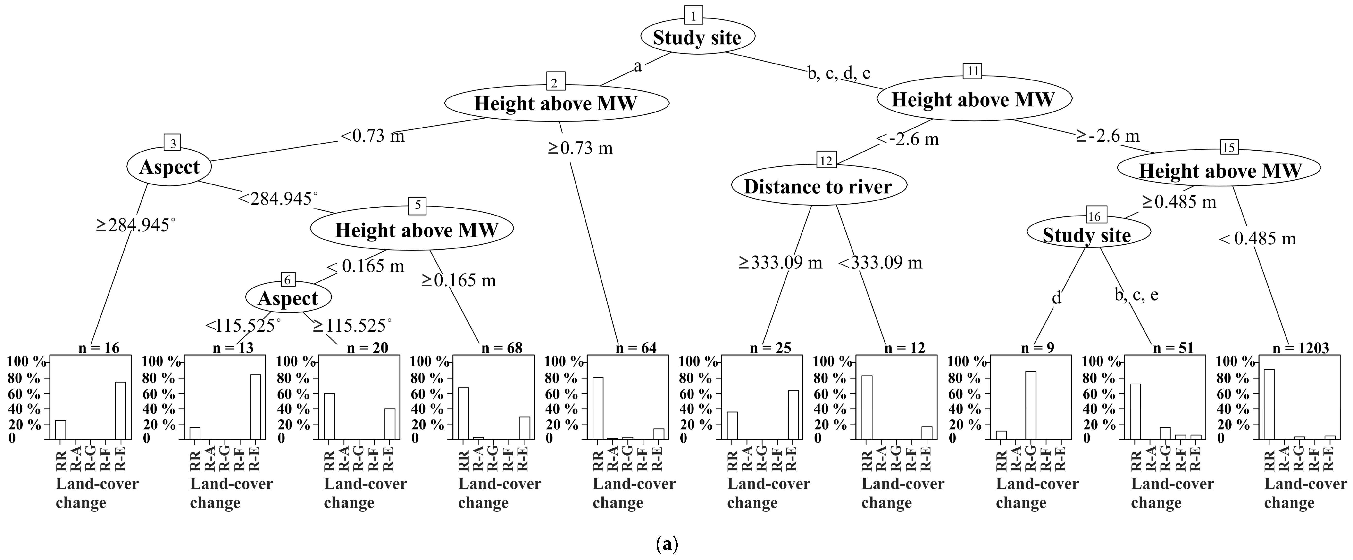
We used the Classification and Regression Tree Model (CART) to explore the relationship between environmental factors and land cover change. CART is a non-parametric method recursively partitioning the dataset of the response variable into homogeneous nodes, and the result is a decision tree [68]. All study sites were rasterized into pixels, and every pixel was characterized by environmental properties. Land cover change was the categorical response variable and environmental parameters were explanatory variables. We ran the CART model for each period of the land cover change of arable land (A), grassland (G), and riparian forest (R) both in active and former floodplains. All other forests and copse were summarized to group F, and all the other land cover types into group E (else). We selected fifteen types of land cover change from twenty-five possible changes based on the habitats of size importance (Table A1). The CART model was calculated using the R package ‘rpart’ [69]. ‘gini’ was selected as the split index, the complexity parameter (CP) was set to 0.01, and the number of cross-validations was defined as 10. The CART model provides the relative variable importance (summing up to 100) to represent the variable influences.
Based on the review of existing studies, the main natural factors of land cover change are slope gradient, altitude, and soil characteristics [70,71]. Considering the dynamic characteristic of the floodplain, we expected that the topographic parameters (slope, aspect), the height above MW (mean water level), the distance to river and the soil parameters could be environmental factors related to the land cover change in this study. The study site was one variable for site differences. All the environmental factors were regarded as stable variables without temporal changes. Elevation, slope and aspect were extracted from the 10-m DEM. The MW data (provided by BfG) were given as height a.s.l. and represented the long-term mean water level of observation sites along the river. Height above MW was the difference between the absolute elevation a.s.l. and the mean annual water level. Distance to river was the distance from the pixel center to the center line of the river. The soil rating index and soil texture were derived from the German Soil Rating Survey (digital soil data was provided by LDBV). The soil rating index is an index with which soil productivity is rated by a single value between 0 and 100, originally surveyed for taxation purposes in Germany [72]. This index is only applied to agricultural land because it is an index evaluating agricultural productivity and is hence missing for forested land and the river. However, we kept the soil rating index in the correlation analysis because it is an important indicator of soil productivity and yield potential [73]. Besides that, the soil rating index correlates reasonably well with soil physical parameters including the clay content and the amount of organic substances [74]. The main soil textures in the study area are S (sand), Sl & lS (loamy sand), SL (very loamy sand), sL (sandy loam), L (loam) and MoL (moor/loam, soil consisting of peat and loam). Among the soil types in the study area, Leptosols and Regosols are formed on the more sandy soils, whereas Gleysols and Luvisols develop on the more loamy soils. Other soil parameters (e.g., organic matter, nutrient levels) could not be considered because these data are not available for the past. Soil texture and study site are categorical variables while all other variables are numeric. The CART method is robust to handle both variable types [68].
3. Results
3.1. Land Cover Change
The largest land cover type both in active and former floodplains is arable land (Figure A1). Although arable land in the active floodplain decreased during all periods, it still occupied the highest share (28.3%) in 2010. It was followed by grassland (15.6%), riparian forest (15.1%) and backwater (14.8%). Common characteristics of all land cover types in the active and the former floodplain are: Between 1963 and 2010 riparian forest increased while arable land and grassland declined. Grassland in the active floodplain decreased during all analyzed time spans. Grassland in the former floodplain decreased by 47%, and was therefore the land cover type with the strongest decline (Table 4). Built-up land and margin increased from 1963 to 1995 and then declined. Woody vegetation including riparian forest and other forest increased by 47% in the active floodplain and doubled in the former floodplain from 1963 to 2010. The area of riparian forest rose from 1963 to 1995, whereas in the last period it declined in most of the study sites (except Barbing).The percentage of agricultural land decreased from 1963 to 2010, while riparian forest increased.
In the active floodplain, all linear structures except field hedge increased from 1963 to 2010, while in the former floodplain, only road, path and margin increased. Path with vegetation experienced an obvious decline from 1978 to 1995, by contrast, paved path increased. The urbanized land cover—settlements, road and path—increased apparently in the former floodplain. There were relatively few roads in the study area, and their increase was accompanied with more road edges. Backwater in study site Barbing increased from 1963 to 1978 due to the creation of a backwater close to the river channel (Figure A1a). The increase of backwater from 1995 to 2010 in study site Gmünd resulted from the high water level and a small flooding event in 2010 (Figure A1b). Overall, the major changes in the active floodplain occurred in arable land, grassland, riparian forest and backwater. In contrast, in the former floodplain, built-up land experienced distinct increases.
The change maps in all study sites depict the overall trend in the land cover change between 1963 and 2010 (Figure 3). The transformation matrix indicates the main changes between arable land, grassland and riparian forest (Table 5). One finding from the transformation matrix is that grassland in the active floodplain always changed into riparian forest or arable land.
The area of grassland changing to riparian forest and the area of arable land transforming into grassland decreased during all the periods. In contrast, in the former floodplain, the conversion between arable land and grassland decreased (Table 5). The transformation percentage of grassland to arable land in the active floodplain increased in the second period and then decreased.
3.2. Structural Change of Land Cover
3.2.1. Landscape Level
In the ANOVA of the landscape metrics, some metrics differ significantly between the active and former floodplain (Table 6). The fragmentation of arable land changed significantly over time (Table 6). Although the structural metrics of riparian forest and grassland did not change significantly in the overall area, the changes occurring in some of the study sites are obvious. In the active floodplain, the shape complexity of the landscape was reduced from 1963 to 1978, it stagnated in the second period, and then the reduction continued from 1995 to 2010 (Table 6). In the active and former floodplain parts the landscape experienced a fragmentation from 1963 to 1995 in Barbing and Gmünd (Figure A1a,b). Although fragmentation decreased in recent years, the landscape in the former floodplain in Barbing, Gmünd, Irlbach and Niederalteich (Figure A1a–d) was still more fragmented in 2010 than in 1963. The diversity of land cover in the active and former floodplain in Barbing and Gmünd increased (Table 6). Landscape shape in the former floodplain in Barbing, Gmünd and Irlbach (Figure A1a–c) became more complex in early periods but then the shape complexity decreased slightly from 1995 to 2010.
3.2.2. Class Level
The patches of the class level ‘arable land’ had a more regular shape in the active floodplain in Barbing, Irlbach, Langkünzing (Figure A1a,c,e). Arable land had a more complex shape in the former than in the active floodplain, but the shape complexity decreased with time in Gmünd and Niederalteich (Table 6, Figure A1b,d). The change of MESH showed a strong fragmentation of arable land in Barbing, Gmünd, Niederalteich and Langkünzing (Figure A1a,b,d,e) from 1978 to 1995, but then this trend was reduced. Compared to the situation in 1963, arable land in the floodplains in Barbing, Gmünd and Niederalteich (Figure A1a,b,d) became more fragmented in 2010. The patches of arable land in the active and former floodplain in all study sites became significantly larger all the time (Figure A1). The patches were closer to each other in the former floodplain in Barbing, Irlbach and Langkünzing in the first period, but from the 1970s to the 1990s this trend was reversed, and afterwards the proximity continued to increase.
The shape complexity of grassland decreased in the active floodplain and grassland patches in the active floodplain in Barbing, Gmünd, Irlbach and Langkünzing (Figure A1a–c,e) became larger. The grassland structure was more fragmented in Barbing, Niederalteich and Langkünzing (Figure A1a,d,e) from 1963 to 1978, but in the next periods it recovered gradually (Table 6). The grassland patches of the former floodplain in Irlbach, Niederalteich and Langkünzing (Figure A1c–e) became more regular in shape. They had no obvious change in average size but became organized. Grassland in the former floodplain in Barbing, Gmünd, Irlbach, Langkünzing experienced a fragmentation, and the patches in Barbing, Irlbach, Niederalteich and Langkünzing diverged more from each other than in 1963 (Table 6).
The shape complexity of riparian forest in the active floodplain in Irlbach and Niederalteich (Figure A1c,d) declined continuously. The patches in Gmünd, Niederalteich and Langkünzing (Figure A1b,d,e) became larger at first, but later slightly smaller (Table 6). In the active floodplain riparian forest tended toward a more aggregated structure in all study sites from 1978 to 1995 and it continued in Barbing, Irlbach and Niederalteich after 1995. The proximity of patches in Gmünd and Niederalteich (Figure A1b,d) was enhanced from 1963 to 1995, in the last period it went through a fall, but the final proximity was higher than that in 1963. The patch size of the riparian forest (in the former floodplain this refers to forests close to water bodies) was larger in the first period, and then with a small fluctuation it was larger in 2010 than the starting state in Barbing, Gmünd and Niederalteich (Figure A1a,b,d).
3.3. Relationship between the Change of Land Cover and Environmental Factors
To have an intuitive impression of the relationship between the environmental factors and the land cover changes, we show the CART results of riparian forest and grassland from 1963 to 1978 exemplarily (Figure 4 and Figure 5). Most riparian forest in the active floodplain of study sites Irlbach, Niederalteich and Langkünzing stayed stable from 1963 to 1978 (Figure 4). In study sites Barbing and Gmünd, riparian forest located higher than about 1 m below MW remained stable. Among the riparian forest lower than 1 m below MW, those forests with a northeast orientation and further than approximately 500 m to the river were converted to grassland; the rest did not change.
In the active floodplain of study sites Gmünd, Irlbach and Langkünzig, most grassland stayed stable from 1963 to 1978 and only a small proportion of grassland with soil consisting of peat and loam converted into arable land (Figure 5). In the active floodplain of study sites Barbing and Niederalteich, grassland with higher soil rating indexes changed into arable land; grassland with lower soil rating indexes became riparian forest; grassland with medium soil rating indexes and closer to the river persisted. As expected, patches farther away from the river are more likely to change into arable land.
In this study, elevation and distance to river were the most important environmental factors to land cover change in the floodplain. The most relevant environmental factors for arable land and grassland changes are soil rating index, height above MW and distance to river; for riparian forest and other woodland, the most important factors are height above MW and distance to river (Table 7). The high values for ‘study site’ showed different trends between study sites (see Figure A3, Figure A4 and Figure A5).
4. Discussion
4.1. How Did the Floodplain Land Cover Change?
The increasing patch size of agricultural land in this study is consistent with comparative studies in Germany, in which many small grassland patches were merged after 1953 [75]. It reflects agricultural intensification with new technical and production methods. Meeus [76] and Hietel et al. [70] showed the trend in agriculture to either intensification or abandonment. While less productive agricultural areas got abandoned, fertile areas were used more intensively. This process started in the 1970s by the Land Consolidation Act in Germany to enhance the agricultural efficiency and reduce the fragmentation with redistribution of small non-adjacent fields between farmers. This action lowered agricultural land division and enlarged the farm size [77]. The observed increase of riparian forest especially close to the river and in low heights above MW indicated that agricultural land use near the river became de-intensified, because high water levels threaten the field cultivation.
The core area and proportion of agricultural land decreased in the active and the former floodplain. In general, the loss of agricultural land could be explained by the German agricultural policy. Since 1962, German agriculture has been under the instruction of EU’s Common Agriculture Policy (CAP) to provide affordable food and to improve the living standard of the farmers [78]. The CAP has contributed to the large-scale land cover change in the past decades [79]. Land cover change in this study was partly related to this development. To enhance the production level was the main focus of the CAP until 1984. Then the measures were adjusted because of the excessive production (e.g., dairy products) above the market demand. After 1992, the farmers were supported with direct aid payments to work more environmentally friendly [80]. Since 2003, with more emphasis on biodiversity conservation, water management and soil protection, the CAP has provided the farmers with income support and motivated them to adopt sustainable agricultural practices [79]. From 2007 to 2013, the Bavarian Cultural Landscape Program (KULAP) provided the farmers with subsidies for the afforestation on agricultural land [81]. In this study, despite the high soil fertility, part of the agricultural land was transformed into riparian forest due to the unreliable water conditions in the floodplain. Nevertheless, the agricultural land still maintained a high share in the active floodplain, which is ecologically negative for the floodplain [82].
Besides the specific land cover change, the floodplain landscape in some study sites experienced a strong fragmentation despite the slight improvement in the active floodplain after 1995. It was shown that the increasing landscape fragmentation in Central Europe was a consequence of patchwork conversion, site development, increasing infrastructure land [62] and water engineering [83]. In this study, the increase of linear structures (road and path) contributed to the increase of shape complexity and landscape fragmentation. The transportation lines can interrupt the natural disturbance regime and lead to the degradation of floodplain habitats, as was found by Blanton and Marcus [84].
4.2. Did the Grassland in the Study Area Decrease?
The area of grassland decreased continuously during the last decades, because grassland was transformed into arable land and riparian forest. Species-rich meadows along the Upper Rhine River have been transformed into arable land since the Middle Ages [85]. The transformation of permanent grassland into arable land due to land-use intensification was also a contributor to the decrease of grassland in the studies by Walz [75] and Tscharntke et al. [86]. Besides land-use intensification, the CAP also stimulated the loss of grassland (see Section 4.1).
Given the importance of grassland in ruminant livestock production, grassland change was partly in line with the variation of livestock number, as discussed by Chang et al. [87] in their work on grassland productivity and ruminant livestock density in Europe. The agricultural statistics in all municipalities within the study area (Figure A2) provided by the Bavarian State Office for Statistics (LfStat) showed an increasing cattle number from 1963 to 1978 and a decrease from 1978 to 2010. Up to 1970 cattle stayed in summer on pastures and were additionally fed with grass and in winter with hay (additional mash), which caused high grass consumption. From 1970 green maize (silage) became the important forage and the demand for arable fields rather than grassland increased. Since the 1980s, dairy products have been reduced, and the cattle number decreased. The decline of livestock production and a preference for market crop production contributed to the transformation from grassland to arable land. As a consequence, the agricultural intensification weakened the grassland demand [7].
Habitat loss and fragmentation reduce the grassland connectivity. The change of connectivity is a crucial aspect of land cover change and implies the spatial alteration of habitat continuity [88]. In this study, the decrease of proximity between grassland patches in most study sites implicates the loss of connectivity. Besides that, margins such as ‘field margin’ and ‘path with vegetation’ were gone, together with their ecological functions, e.g., as migration corridor and for biodiversity enhancement.
4.3. Did the Riparian Forest in the Study Area Decrease?
Although the riparian forest decreased overall in the time span between 1995 and 2010, the total area of riparian forest increased up to now. Riparian forest change varies worldwide. Due to hydroelectric power stations and other management measures, the Rhine Alsatian forest and the Austrian forest along the Danube River decreased by 25–50% from the 1930s to 1980s [82]. The cumulative loss of riparian forest was driven by dam construction, intensive agriculture (enhancement of maize production on former grassland sites), urban development, forest management and timber harvesting [83]. In our study region, the river engineering projects between Straubing and Vilshofen from the 1990s had strong influences on the floodplain habitats. The flood protection measures led to the change of site parameters including depth to groundwater level, groundwater fluctuations and flow rate. They further resulted in a loss of area for natural development. Some parts of the forested area in the floodplain shifted to the water zone or even open water area [89].
The main increase of riparian forest area in this study originated from the transformation from grassland and arable land. This could be explained by land-use policy change in Western Europe (foundation of EWG in 1957, EU in 1993). The CAP supported the afforestation of agricultural land, and this gave rise to an increase of 4.9% forest in the Federal Republic of Germany from 1950 to 1993 [90]. This afforestation compensated clear cuttings and led to an increase of the forest cover [91]. In this study, riparian forest in most study sites became more aggregated in the last 50 years. Forest patches grew larger from 1963 to 1995 in the active floodplain, and the patch shape was more regular than before. In contrast, floodplain forests along other large rivers (e.g., the Upper Rhine River) have experienced strong fragmentation in the last decades [82].
In German floodplain management practices, to ensure the flood retention, riparian forest was removed to decrease the roughness and increase the water velocity. Since 2004, management measures including the thinning of softwood stocks have been taken in the Danube Waterway Project between Straubing and Vilshofen [92]. However, in forest restoration projects along the Middle Elbe River, it was shown that forest plantings in suitable positions can help to control flooding. Due to the increased roughness in the planted forests, water is kept in areas designated for flood retention. Flood waves are flattened and flood-sensitive areas are secured. This form of landscape management is a solution for the conflicts between natural conservation and flood protection [22], but due to the high population density and limited amount of space along the Upper Danube River, this measure is probably not suitable in our study area.
4.4. Suitability of Landscape Structure Analysis
Landscape metrics were used to analyze the land cover pattern and to quantify the fragmentation. As a prerequisite to the study of landscape function and change, much effort has been put into calculating the landscape metrics to quantify the landscape structure in previous studies [93]. However, these metrics have to be selected and interpreted in relation to their ecological meaning [94]. Without supporting data on species level, only general landscape patterns and processes can be pointed out.
We selected the landscape metrics in consideration of their ecological meanings. Effective mesh size (MESH) and edge density are measures to quantify the fragmentation, which affects processes like animal dispersion and habitat viability [95]. The increase of MESH indicated the more aggregated structure of riparian forest, which benefits the species that are sensitive to edge effects [57]. The shape index indicating the shape complexity of the forest affects the bird abundance [57]. The shape of habitat fragments also influences animal population dynamics and meta-population persistence within fragments [96].
Even though it is not possible to draw conclusions on specific ecological processes or the effects of changes on single species groups [93], the analysis of landscape metrics gives information about the changes in landscape structure and landscape structural composition over time and the general effects of these changes. Suitable landscape metrics that are easy to interpret by stakeholders and decision-makers who are responsible for planning and management can help to increase the understanding for landscape structural and functional patterns.
4.5. Relationship between Grassland and Riparian Forest Change and Environmental Factors
For the agricultural land cover change, soil quality played the most important role. The importance of the variable ‘study site’ implied different changes between study sites. Previous researchers found that land cover changes in submontane landscapes of Germany were correlated with physical landscape attributes, e.g., elevation, slope, aspect, water capacity and soil texture [70,97]. Other studies reported the importance of relief, hydrological and soil conditions in the active floodplain: the principal environmental gradients: hydroperiod, the depth of the groundwater table and soil fertility determine water → plant → soil interactions [98]. Height above MW is related to hydrological differences. Higher sites in the floodplain are much drier than lower sites because they are farther from the groundwater table. Distance to river is a significant factor for the spatial variability in the depth and duration of inundation, soil properties, nutrient accumulation and other ecological processes in the floodplain [99]. Bürgi and Turner [100] detected different land cover changes in various soil conditions: agricultural land changed into forest as a result of agricultural abandonment on shallow soils; arable land changed into grassland due to the decline of farming intensity on more sandy and deeper soils; fertile grassland sites on silty soils were transformed into arable land owing to agricultural intensification. Along many European rivers, the original floodplain forests were cleared for agricultural production on fertile soils [82]. In the present study, grassland in the active floodplain with higher soil rating indexes changed into arable land, while grassland with lower soil rating indexes tended to change into riparian forest, which confirmed less preference of agricultural production on these soils. The farmers tend to convert the grassland with higher productivity into arable land to improve the agricultural production. In this study riparian forest change was mainly related with height above MW and distance to river. The flood-dependent attributes and the preference for high groundwater level of riparian forest allowed these sites to develop into forest [2].
4.6. What Is the Ecological Relevance of the Observed Trends in the Floodplain?
The decline of agricultural land and the increase of riparian forest compared to the original state positively affect the floodplain. As a natural habitat, riparian forest is of high importance in river-floodplain ecosystems. It can reduce the sediment amount in the river and help to mitigate the flood risk [101]. The clearance of riparian forest for overflow optimization is caused by human population’s demand for safe living conditions, but it should be in harmony with the protection of flora and fauna. The hydraulic roughness of floodplain vegetation could be modeled to see the influences on flood water level and to reinforce coordination between ecosystem rehabilitation and flood safety [102].
On the landscape level, the finding of increasing fragmentation in the floodplain is a warning signal for the loss of biological diversity and ecological functions [103]. In other studies, poor connectivity and strong fragmentation of floodplain result in a lower rate of mineral sedimentation and P accumulation [104]. In this study agricultural intensification shifted the arable land into larger fields, which equalized the conditions and had negative impacts on species diversity, as also found by Harms et al. [105]. Fertilizers and pesticides used in agriculture can lead to groundwater pollution and river eutrophication. The natural forests in floodplains should be protected to provide refuges for species and to improve biodiversity generally [83].
5. Conclusions
In the Upper Danube Floodplain, our study focused on the change of land cover and the relevant environmental factors. The increasing fragmentation of the floodplain landscape was a consequence of the disturbance by water management, agricultural intensification and linear infrastructure. In spite of the decline of agricultural land in the floodplain in recent decades, it still accounted for a large proportion in the active floodplain and agricultural intensification threatened the ecological functions of floodplain habitats. The aggregated structure of riparian forest is likely to have positive influences from an ecological view. However, the trend of increasing riparian forest was relativized by cutting forests for flood protection, Given that the Danube is an important federal waterway, the local water management office made plans to protect the riparian forest and limit the intensive agricultural use in the Danube Floodplain [106]. To achieve a sustainable floodplain development, an agreement between different interests, e.g., shipping traffic, flood protection and nature conservation has to be reached.
Acknowledgments
We would like to thank The German Federal Institute of Hydrology (BfG), the Bavarian State Office for Survey and Geoinformation (LDBV), the Bavarian Environment Agency (LfU) and the Bavarian State Office for Statistics (LfStat) for the provision of data. We are thankful to all colleagues from the Division of Landscape Ecology and Landscape Planning for suggestions and discussion in the research process. This study is funded by a Ph.D. scholarship to Fang Xu awarded by the China Scholarship Council (CSC) and we appreciate the financial support.
Author Contributions
Conceived and designed this study: Fang Xu, Annette Otte, Kristin Ludewig, Tobias W. Donath, Sarah Harvolk-Schöning; Analyzed the data: Fang Xu; Wrote the paper: Fang Xu; Revised the paper: Annette Otte, Kristin Ludewig, Tobias W. Donath and Sarah Harvolk-Schöning. All authors read and approved the final manuscript.
Conflicts of Interest
The authors declare no conflict of interest. The founding sponsors had no role in the design of the study; in the collection, analyses, or interpretation of data; in the writing of the manuscript, and in the decision to publish the results.
Appendix A

Table A1.
Selected types of land cover change of arable land (A), grassland (G) and riparian forest (R).
Table A1.
Selected types of land cover change of arable land (A), grassland (G) and riparian forest (R).
| Abbreviation (Alphabetic Order) | Description |
|---|---|
| AA | Stable arable land |
| A-G | Arable land to grassland |
| A-R | Arable land to riparian forest |
| A-F | Arable land to other forests |
| A-E | Arable land to other land cover |
| GG | Stable grassland |
| G-A | Grassland to arable land |
| G-R | Grassland to riparian forest |
| G-F | Grassland to other forests |
| G-E | Grassland to other land cover |
| RR | Stable riparian forest |
| R-A | Riparian forest to arable land |
| R-G | Riparian forest to grassland |
| R-F | Riparian forest to other forests |
| R-E | Riparian forest to other land cover |
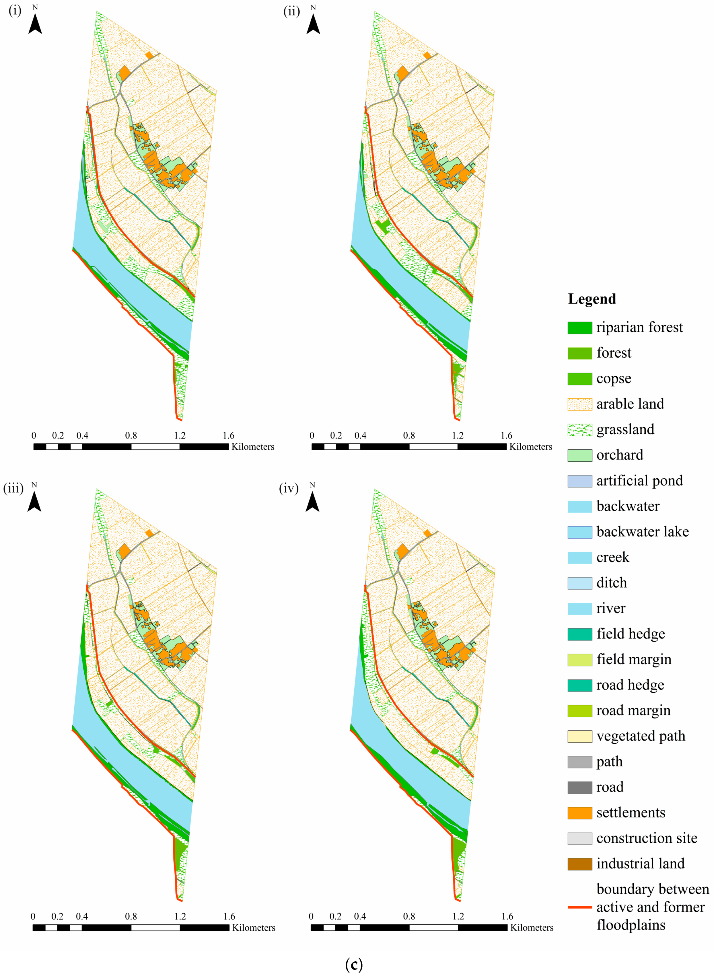
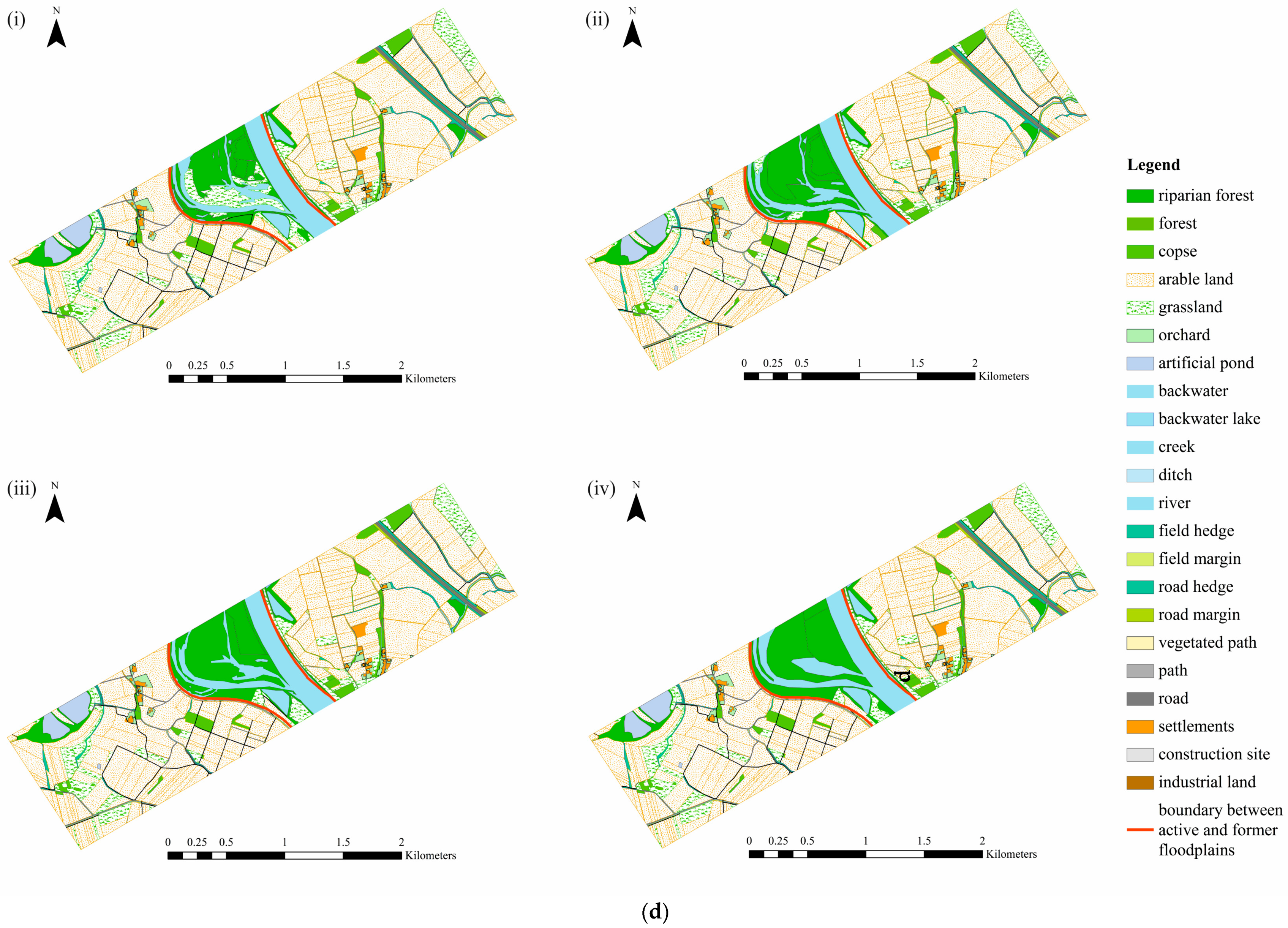
Figure A1.
An overview of land cover structure in the active and former floodplains of all study sites: (a) Barbing; (b) Gmünd; (c) Irlbach; (d) Niederalteich and (e) Langkünzig during all the periods (i. 1963; ii. 1978; iii. 1995; iv. 2010).
Figure A1.
An overview of land cover structure in the active and former floodplains of all study sites: (a) Barbing; (b) Gmünd; (c) Irlbach; (d) Niederalteich and (e) Langkünzig during all the periods (i. 1963; ii. 1978; iii. 1995; iv. 2010).


Figure A2.
The cattle number of 1960, 1979, 1991 and 2010 in all the municipalities of the study area [107]. The small letters refer to the study sites, see Figure 1.

Figure A3.
The CART result of arable land change and environmental factors ((a) 1963–1978; (b) 1978–1995; (c) 1995–2010). Abbreviations: AA: stable arable land; A-G: arable land to grassland; A-R: arable land to riparian forest; A-F: arable land to other forests; A-E: arable land to other land cover; S: sand; Sl & lS: loamy sand; SL: very loamy sand; sL: sandy loam; L: loam; MoL: moor/loam, soil consisting of peat and loam; the small letters refer to the study sites, see Figure 1.


Figure A4.
The CART result of riparian forest change and environmental factors ((a) 1978–1995; (b) 1995–2010). Abbreviations: RR: stable riparian forest; R-A: riparian forest to arable land; R-G: riparian forest to grassland; R-F: riparian forest to other forests; RE: riparian forest to other land cover; the small letters refer to the study sites, see Figure 1.


Figure A5.
The CART result of grassland change and environmental factors ((a) 1978–1995; (b) 1995–2010). Abbreviations: GG: stable grassland; G-A: grassland to arable land; G-R: grassland to riparian forest; G-F: grassland to other forests; G-E: grassland to other land cover; S: sand; Sl & lS: loamy sand; SL: very loamy sand; sL: sandy loam; L: loam; MoL: moor/ loam, soil consisting of peat and loam; the small letters refer to the study sites, see Figure 1.


References
- Härdtle, W. On the theoretical concept of the potential natural vegetation and proposals for an up-to-date modification. Folia Geobot. 1995, 30, 263–276. [Google Scholar] [CrossRef]
- Hughes, F.M.R.; Rood, S.B. Allocation of River Flows for Restoration of Floodplain Forest Ecosystems: A Review of Approaches and Their Applicability in Europe. Environ. Manag. 2003, 32, 12–33. [Google Scholar] [CrossRef] [PubMed]
- Welsch, D.J. Riparian Forest Buffers—Function and Design for Protection and Enhancement of Water Resources; NA-PR-07-91; USDA Forest Service Northeastern Area: Radnor, PA, USA, 1991.
- Schmitt, C.B.; Belokurov, A.; Besançon, C.; Boisrobert, L.; Burgess, N.D.; Campbell, A.; Coad, L.; Fish, L.; Gliddon, D.; Humphries, K.; et al. Global Ecological Forest Classification and Forest Protected Area Gap Analysis. Analyses and Recommendations in View of the 10% Target for Forest Protection under the Convention on Biological Diversity (CBD), 2nd ed.; Freiburg University Press: Freiburg, Germany, 2009; pp. 1–34. [Google Scholar]
- Habel, J.C.; Dengler, J.; Janišová, M.; Török, P.; Wellstein, C.; Wiezik, M. European grassland ecosystems: Threatened hotspots of biodiversity. Biodivers. Conserv. 2013, 22, 2131–2138. [Google Scholar] [CrossRef]
- Krause, B.; Culmsee, H.; Wesche, K.; Bergmeier, E.; Leuschner, C. Habitat loss of floodplain meadows in north Germany since the 1950s. Biodivers. Conserv. 2011, 20, 2347–2364. [Google Scholar] [CrossRef]
- Wesche, K.; Krause, B.; Culmsee, H.; Leuschner, C. Fifty years of change in Central European grassland vegetation: Large losses in species richness and animal-pollinated plants. Biol. Conserv. 2012, 150, 76–85. [Google Scholar] [CrossRef]
- Freeman, R.E.; Stanley, E.H.; Turner, M.G. Analysis and conservation implications of landscape change in the Wisconsin River floodplain, USA. Ecol. Appl. 2003, 13, 416–431. [Google Scholar] [CrossRef]
- Hein, T.; Schwarz, U.; Habersack, H.; Nichersu, I.; Preiner, S.; Willby, N.; Weigelhofer, G. Current status and restoration options for floodplains along the Danube River. Sci. Total Environ. 2016, 543, 778–790. [Google Scholar] [CrossRef] [PubMed]
- Schiemer, F.; Guti, G.; Keckeis, H.; Staras, M. Ecological Status and Problems of the Danube River and its Fish Fauna: A Review. In Proceedings of the Second International Symposium on the Management of Large Rivers for Fisheries, Phnom Penh, Kingdom of Cambodia, 11–14 February 2003; Welcomme, R.L., Petr, T., Eds.; FAO Regional Office for Asia and the Pacific: Bangkok, Thailand, 2004; Volume 1, pp. 273–299. [Google Scholar]
- Schwarz, U. Assessment of the Balance and Management of Sediments of the Danube; Slovenian National Commitee for IHP Unesco: Ljubljana, Slovenia, 2008. [Google Scholar]
- Gingrich, S.; Haidvogl, G.; Krausmann, F. The Danube and Vienna: Urban resource use, transport and land cover 1800–1910. Reg. Environ. Chang. 2012, 12, 283–294. [Google Scholar] [CrossRef]
- Winiwarter, V.; Schmid, M.; Hohensinner, S.; Haidvogl, G. The environmental history of the Danube River Basin as an issue of long-term socio-ecological research. In Long Term Socio-Ecological Research: Studies in Society-Nature Interactions across Spatial and Temporal Scales; Singh, S.J., Haberl, H., Chertow, M., Mirtl, M., Schmid, M., Eds.; Springer: Dordrecht, The Netherlands, 2013; Volume 2, pp. 103–122. [Google Scholar]
- Jungwirth, M. Ecology of Large Rivers, Anthropogenic Pressures and Impacts; ICPDR: Vienna, Austria, 2007; Available online: https://www.icpdr.org/main/sites/default/files/JUNGWIRTH_BOKU_EcologyLargeRivers.pdf (accessed on 11 June 2016).
- Ward, J.V.; Stanford, J.A. Ecological connectivity in alluvial river ecosystems and its disruption by flow regulation. River Res. Appl. 1995, 11, 105–119. [Google Scholar] [CrossRef]
- González, E.; González-Sanchís, M.; Cabezas, Á.; Comín, F.A.; Muller, E. Recent changes in the riparian forests of a large regulated Mediterranean river: Implications for management. Environ. Manag. 2010, 45, 669–681. [Google Scholar] [CrossRef] [PubMed]
- Bloesch, J.; Gutknecht, D.; Iordache, V. (Eds.) Report on the International Workshop “Hydrology and Limnology–Another Boundary in the Danube River Basin”, Petronell, Austria, October 14–16, 2004; International Association for Danube Research (IAD): Vienna, Austria, 2004. [Google Scholar]
- Dale, V.H.; Brown, S.; Haeuber, R.A.; Hobbs, N.T.; Huntly, N.; Naiman, R.J.; Riebsame, W.E.; Turner, M.G.; Valone, T.J. Ecological principles and guidelines for managing the use of land. Ecol. Appl. 2000, 10, 639–670. [Google Scholar] [CrossRef]
- Lindborg, R.; Eriksson, O. Historical landscape connectivity affects present plant species diversity. Ecology 2004, 85, 1840–1845. [Google Scholar] [CrossRef]
- Tilman, D.; May, R.M.; Lehman, C.L.; Nowak, M.A. Habitat destruction and the extinction debt. Nature 1994, 371, 65–66. [Google Scholar] [CrossRef]
- Kuussaari, M.; Bommarco, R.; Heikkinen, R.K.; Helm, A.; Krauss, J.; Lindborg, R.; Öckinger, E.; Pärtel, M.; Pino, J.; Rodà, F.; et al. Extinction debt: A challenge for biodiversity conservation. Trends Ecol. Evol. 2009, 24, 564–571. [Google Scholar] [CrossRef] [PubMed]
- Leyer, I.; Mosner, E.; Lehmann, B. Managing floodplain-forest restoration in European river landscapes combining ecological and flood-protection issues. Ecol. Appl. 2012, 22, 240–249. [Google Scholar] [CrossRef] [PubMed]
- De Jager, N.R.; Rohweder, J.J. Changes in aquatic vegetation and floodplain land cover in the Upper Mississippi and Illinois rivers (1989–2000–2010). Environ. Monit. Assess. 2017, 189, 77. [Google Scholar] [CrossRef] [PubMed]
- Fang, X.Q.; Ren, L.L.; Li, Q.F. The detection and analysis of land use change in the Laoha River Basin during the past four decades. Remote Sens. Land Resour. 2012, 24, 125–131. [Google Scholar]
- Fickas, K.C.; Cohen, W.B.; Yang, Z. Landsat-based monitoring of annual wetland change in the Willamette Valley of Oregon, USA from 1972 to 2012. Wetl. Ecol. Manag. 2016, 24, 73–92. [Google Scholar] [CrossRef]
- Dufour, S.; Rinaldi, M.; Piégay, H.; Michalon, A. How do river dynamics and human influences affect the landscape pattern of fluvial corridors? Lessons from the Magra River, Central–Northern Italy. Landsc. Urban Plan. 2015, 134, 107–118. [Google Scholar] [CrossRef]
- Müller, N. Effects of natural and human disturbances on floodplain vegetation. In Proceedings of the International Symposium on River Restoration, Tokyo, Japan, 26–27 May 1998. [Google Scholar]
- Stromberg, J.C.; Tluczek, M.G.; Hazelton, A.F.; Ajami, H. A century of riparian forest expansion following extreme disturbance: Spatio-temporal change in Populus/Salix/Tamarix forests along the Upper San Pedro River, Arizona, USA. For. Ecol. Manag. 2010, 259, 1181–1189. [Google Scholar] [CrossRef]
- Pechanec, V.; Machar, I.; Kilianová, H. Development of land use in the Morava River Floodplain during the past 175 years. In New Developments in Environmental Science and Geoscience, Proceedings of the International Conference on Environmental Science and Geoscience (ESG 2015), Vienna, Austria, 15–17 March 2015. [Google Scholar]
- Tockner, K.; Pusch, M.; Borchardt, D.; Lorang, M.S. Multiple stressors in coupled river–floodplain ecosystems. Freshw. Biol. 2010, 55, 135–151. [Google Scholar] [CrossRef]
- Hudson, P.F.; Colditz, R.R.; Aguilar-Robledo, M. Spatial relations between floodplain environments and land use-land cover in a large lowland tropical river valley: Pánuco basin México. Environ. Manag. 2006, 38, 487–503. [Google Scholar] [CrossRef] [PubMed]
- Herold, M.; Goldstein, N.C.; Clarke, K.C. The spatiotemporal form of urban growth: Measurement, analysis and modeling. Remote Sens. Environ. 2003, 86, 286–302. [Google Scholar] [CrossRef]
- Cushman, S.A.; McGarigal, K. Landscape metrics, scales of resolution. In Designing Green Landscapes; Gadow, K., Pukkala, T., Eds.; Springer: Dordrecht, The Netherlands, 2008; pp. 33–51. [Google Scholar]
- Fichera, C.R.; Modica, G.; Pollino, M. Land Cover classification and change-detection analysis using multi-temporal remote sensed imagery and landscape metrics. Eur. J. Remote Sens. 2012, 45, 1–18. [Google Scholar] [CrossRef]
- Schindler, S.; von Wehrden, H.; Poirazidis, K.; Wrbka, T.; Kati, V. Multiscale performance of landscape metrics as indicators of species richness of plants, insects and vertebrates. Ecol. Indic. 2013, 31, 41–48. [Google Scholar] [CrossRef]
- Lausch, A.; Herzog, F. Applicability of landscape metrics for the monitoring of landscape change: Issues of scale, resolution and interpretability. Ecol. Indic. 2002, 2, 3–15. [Google Scholar] [CrossRef]
- Zhao, Q.; Liu, S.; Deng, L.; Dong, S.; Yang, Z.; Yang, J. Landscape change and hydrologic alteration associated with dam construction. Int. J. Appl. Earth Obs. Geoinf. 2012, 16, 17–26. [Google Scholar] [CrossRef]
- Fox, D.M.; Witz, E.; Blanc, V.; Soulié, C.; Penalver-Navarro, M.; Dervieux, A. A case study of land cover change (1950–2003) and runoff in a Mediterranean catchment. Appl. Geogr. 2012, 32, 810–821. [Google Scholar] [CrossRef]
- Merritt, D.M.; Poff, N. Shifting dominance of riparian Populus and Tamarix along gradients of flow alteration in western North American rivers. Ecol. Appl. 2010, 20, 135–152. [Google Scholar] [CrossRef] [PubMed]
- Benjankar, R.; Egger, G.; Jorde, K.; Goodwin, P.; Glenn, N.F. Dynamic floodplain vegetation model development for the Kootenai River, USA. J. Environ. Manag. 2011, 92, 3058–3070. [Google Scholar] [CrossRef] [PubMed]
- Ward, J.V.; Tockner, K.; Arscott, D.B.; Claret, C. Riverine landscape diversity. Freshw. Biol. 2002, 47, 517–539. [Google Scholar] [CrossRef]
- Schweizer, P.E.; Matlack, G.R. Factors driving land use change and forest distribution on the coastal plain of Mississippi, USA. Landsc. Urban Plan. 2014, 121, 55–64. [Google Scholar] [CrossRef]
- Jung, M.; Burt, T.P.; Bates, P.D. Toward a conceptual model of floodplain water table response. Water Resour. Res. 2004, 40. [Google Scholar] [CrossRef]
- Butler, J.R.; Wong, G.Y.; Metcalfe, D.J.; Honzák, M.; Pert, P.L.; Rao, N.; van Grieken, M.E.; Lawson, T.; Bruce, C.; Kroon, F.J.; et al. An analysis of trade-offs between multiple ecosystem services and stakeholders linked to land use and water quality management in the Great Barrier Reef, Australia. Agric. Ecosyst. Environ. 2013, 180, 176–191. [Google Scholar] [CrossRef]
- Jones, K.B.; Slonecker, E.T.; Nash, M.S.; Neale, A.C.; Wade, T.G.; Hamann, S. Riparian habitat changes across the continental United States (1972–2003) and potential implications for sustaining ecosystem services. Landsc. Ecol. 2010, 25, 1261–1275. [Google Scholar] [CrossRef]
- Schmidt, H.G. Postwar Developments in West German Agriculture, 1945–1953. Agric. Hist. 1955, 29, 147–159. [Google Scholar]
- Marggraf, R. Comparative assessment of agri-environment programmes in federal states of Germany. Agric. Ecosyst. Environ. 2003, 98, 507–516. [Google Scholar] [CrossRef]
- Schneider, E. Floodplain restoration of large European rivers, with examples from the Rhine and the Danube. In Restoration of Lakes, Streams, Floodplains, and Bogs in Europe, 1st ed.; Eiseltová, M., Ed.; Springer: Dordrecht, The Netherlands, 2010; pp. 185–223. [Google Scholar]
- International Commission for the Protection of the Danube River (ICPDR). Danube Facts and Figures: Germany; ICPDR: Vienna, Austria, 2007; Available online: https://www.icpdr.org/main/sites/default/files/DE_Facts_%20Figures.pdf (accessed on 16 May 2016).
- Bavarian Environment Agency (LfU). Description of the Cultural Landscape 33 Dungau. In Draft of the Structure of the Bavarian Cultural Landscape as a Contribution to Biodiversity; Bavarian Environment Agency (LfU): Augsburg, Germany, 2011; Available online: http://www.lfu.bayern.de/natur/kulturlandschaft/entwurf_gliederung/doc/33_dungau.pdf (accessed on 16 May 2016). (In German)
- German Meteorological Service (DWD). Long-Term Mean Values for Reference Period 1981–2010, Precipitation and Temperature Raster Map for Germany. Offenbach, Germany, 2013. Available online: www.dwd.de (accessed on 16 May 2016).
- Seibert, P. Overview Map of Natural Vegetation Area of Bayern 1: 500,000 with Explanations, Series for Vegetation Science; The German Federal Agency for Nature Conservation (BfN): Bad Godesberg, Germany, 1968; Volume 3. (In German) [Google Scholar]
- Bavarian State Office for Survey and Geoinformation (LDBV). Digital Orthophotos (DOP 20), Ground Resolution: 0.2 m × 0.2 m; Bavarian State Office for Survey and Geoinformation (LDBV): Munich, Germany, 2014. [Google Scholar]
- Djebou, D.C.S. Integrated approach to assessing streamflow and precipitation alterations under environmental change: Application in the Niger River Basin. J. Hydrol. Reg. Stud. 2015, 4, 571–582. [Google Scholar] [CrossRef]
- Long, H.; Tang, G.; Li, X.; Heilig, G.K. Socio-economic driving forces of land-use change in Kunshan, the Yangtze River Delta economic area of China. J. Environ. Manag. 2007, 83, 351–364. [Google Scholar] [CrossRef] [PubMed]
- Uuemaa, E.; Mander, Ü.; Marja, R. Trends in the use of landscape spatial metrics as landscape indicators: A review. Ecol. Indic. 2013, 28, 100–106. [Google Scholar] [CrossRef]
- Ewers, R.M.; Didham, R.K. The effect of fragment shape and species’ sensitivity to habitat edges on animal population size. Conserv. Biol. 2007, 21, 926–936. [Google Scholar] [CrossRef] [PubMed]
- Moser, D.; Zechmeister, H.G.; Plutzar, C.; Sauberer, N.; Wrbka, T.; Grabherr, G. Landscape patch shape complexity as an effective measure for plant species richness in rural landscapes. Landsc. Ecol. 2002, 17, 657–669. [Google Scholar] [CrossRef]
- McGarigal, K.; Marks, B.J. Fragstats: Spatial Pattern Analysis Program for Quantifying Landscape Structure; Gen. Tech. Rep. PNW-GTR-351; USDA Forest Service Pacific Northwest Research Station: Portland, OR, USA, 1995.
- Didham, R.K. Ecological Consequences of Habitat Fragmentation. Available online: http://www.els.net/WileyCDA/ElsArticle/refId-a0021904.html (accessed on 1 June 2017).
- Rutledge, D. Landscape Indices as Measures of the Effects of Fragmentation: Can Pattern Reflect Process? DOC Science Internal Series 98; Department of Conservation: Wellington, New Zealand, 2003.
- Jaeger, J.A. Landscape division, splitting index, and effective mesh size: New measures of landscape fragmentation. Landsc. Ecol. 2000, 15, 115–130. [Google Scholar] [CrossRef]
- Gustafson, E.J.; Parker, G.R. Using an index of habitat patch proximity for landscape design. Landsc. Urban Plan. 1994, 29, 117–130. [Google Scholar] [CrossRef]
- Bender, D.J.; Tischendorf, L.; Fahrig, L. Using patch isolation metrics to predict animal movement in binary landscapes. Landsc. Ecol. 2003, 18, 17–39. [Google Scholar] [CrossRef]
- Peters, D.P.; Goslee, S.C. Landscape diversity. Encycl. Biodivers. 2001, 3, 645–658. [Google Scholar] [CrossRef]
- Fahrig, L.; Baudry, J.; Brotons, L.; Burel, F.G.; Crist, T.O.; Fuller, R.J.; Sirami, C.; Siriwardena, G.M.; Martin, J.L. Functional landscape heterogeneity and animal biodiversity in agricultural landscapes. Ecol. Lett. 2011, 14, 101–112. [Google Scholar] [CrossRef] [PubMed]
- Nagendra, H. Opposite trends in response for the Shannon and Simpson indices of landscape diversity. Appl. Geogr. 2002, 22, 175–186. [Google Scholar] [CrossRef]
- Lewis, R.J. An introduction to classification and regression tree (CART) analysis. In Proceedings of the Annual Meeting of the Society for Academic Emergency Medicine, San Francisco, CA, USA, 22–25 May 2000; pp. 1–14. [Google Scholar]
- Therneau, T.; Atkinson, B.; Ripley, B. Package ‘rpart’: Recursive Partitioning and Regression Trees. R Package Version 4.1–10. 2015. Available online: https://cran.r-project.org/web/packages/rpart/index.html (accessed on 16 May 2016).
- Hietel, E.; Waldhardt, R.; Otte, A. Analysing land cover changes in relation to environmental variables in Hesse, Germany. Landsc. Ecol. 2004, 19, 473–489. [Google Scholar] [CrossRef]
- Opršal, Z.; Šarapatka, B.; Kladivo, P. Land-use changes and their relationships to selected landscape parameters in three cadastral areas in Moravia (Czech Republic). Morav. Geogr. Rep. 2013, 21, 41–50. [Google Scholar] [CrossRef]
- Rothkegel, W.; Herzog, H. The Soil Evaluation Law—Comment; Carl Heymanns: Berlin, Germany, 1935. (In German) [Google Scholar]
- Breitschuh, G.; Eckert, H.; Breitschuh, T.; Körschens, M. Soil fertility in sustainable agriculture. In Soil Fertility-Basis of Successful Agriculture, Proceedings of the Conference of the Association of Agricultural Chambers (VLK) and the Federal Working Group on Fertilization (BAD), Würzburg, Germany, 21–22 April 2015. (In German). [Google Scholar]
- Vorderbrügge, T.; Miller, R.; Peter, M.; Sauer, S. Derivation of soil-physical parameters from the class indexes of soil evaluation using the example of the field capacity. DBG-Mitteilungen 2005, 107, 531–532. (In German) [Google Scholar]
- Walz, U. Monitoring of landscape change and functions in Saxony (Eastern Germany)–Methods and indicators. Ecol. Indic. 2008, 8, 807–817. [Google Scholar] [CrossRef]
- Meeus, J.H.A. Pan-European landscapes. Landsc. Urban Plan. 1995, 31, 57–79. [Google Scholar] [CrossRef]
- Thomas, J. Property rights, land fragmentation and the emerging structure of agriculture in Central and Eastern European countries. J. Agric. Dev. Econ. 2006, 3, 225–275. [Google Scholar]
- European Commission. The Common Agricultural Policy: A Partnership between Europe and Farmers; Publications Office of the European Union: Luxembourg, Luxembourg, 2014; pp. 1–16. Available online: http://www.euic.mk/content/Brochures-pdf-NEW/EN/Agriculture_EN.pdf (accessed on 19 August 2016).
- Henle, K.; Alard, D.; Clitherow, J.; Cobb, P.; Firbank, L.; Kull, T.; McCracken, D.; Moritz, R.F.A.; Niemelä, J.; Rebane, M.; et al. Identifying and managing the conflicts between agriculture and biodiversity conservation in Europe—A review. Agric. Ecosyst. Environ. 2008, 124, 60–71. [Google Scholar] [CrossRef]
- Parris, K. Measuring the environmental impacts of the common agricultural policy: Challenges, recent trends and outlook, and future directions. In Proceedings of the Common Agriculture Policy and the Environmental Challenge—New Tasks for the Public Administrations, Maastricht, The Netherlands, 14–15 May 2001. [Google Scholar]
- Bavarian State Ministry of Food, Agriculture and Forestry (StMELF) & Bavarian State Ministry of the Environment and Consumer Protection (StMUV). Bavarian Future Program Agriculture and Rural Areas 2007–2013; Bavarian State Ministry of Food, Agriculture and Forestry (StMELF) & Bavarian State Ministry of the Environment and Consumer Protection (StMUV): Munich, Germany, 2005; pp. 1–849. (In German) [Google Scholar]
- Klimo, E.; Hager, H. The Floodplain Forests in Europe: Current Situations and Perspectives; European Forest Institute Research Report 10; Brill: Leiden, The Netherlands, 2001. [Google Scholar]
- Schnitzler, A.; Hale, B.W.; Alsum, E. Biodiversity of floodplain forests in Europe and eastern North America: A comparative study of the Rhine and Mississippi Valleys. Biodivers. Conserv. 2005, 14, 97–117. [Google Scholar] [CrossRef]
- Blanton, P.; Marcus, W.A. Transportation infrastructure, river confinement, and impacts on floodplain and channel habitat, Yakima and Chehalis rivers, Washington, USA. Geomorphology 2013, 189, 55–65. [Google Scholar] [CrossRef]
- Dister, E.; Gomer, D.; Obrdlik, P.; Petermann, P.; Schneider, E. Water management and ecological perspectives of the Upper Rhine’s floodplains. River Res. Appl. 1990, 5, 1–15. [Google Scholar] [CrossRef]
- Tscharntke, T.; Klein, A.M.; Kruess, A.; Steffan-Dewenter, I.; Thies, C. Landscape perspectives on agricultural intensification and biodiversity – ecosystem service management. Ecol. Lett. 2005, 8, 857–874. [Google Scholar] [CrossRef]
- Chang, J.; Viovy, N.; Vuichard, N.; Ciais, P.; Campioli, M.; Klumpp, K.; Martin, R.; Leip, A.; Soussana, J.F. Modeled Changes in Potential Grassland Productivity and in Grass-Fed Ruminant Livestock Density in Europe over 1961—2010. PLoS ONE 2015, 10, e0127554. [Google Scholar] [CrossRef] [PubMed]
- Soons, M.B.; Messelink, J.H.; Jongejans, E.; Heil, G.W. Habitat fragmentation reduces grassland connectivity for both short-distance and long-distance wind-dispersed forbs. J. Ecol. 2005, 93, 1214–1225. [Google Scholar] [CrossRef]
- German Federal Institute of Hydrology (BfG). Vegetation of the Danube Floodplain between Straubing and Vilshofen—Site Potential for Floodplain Vegetation of the Actual Situation and the Design Variants; BfG-1773; BfG: Koblenz, Germany, 2012. (In German) [Google Scholar]
- Sayer, J.A.; Maginnis, S. Forests in Landscapes: Ecosystem Approaches to Sustainability; Routledge: London, UK, 2007. [Google Scholar]
- Mikusiński, G.; Angelstam, P. Economic geography, forest distribution, and woodpecker diversity in Central Europe. Conserv. Biol. 1998, 12, 200–208. [Google Scholar] [CrossRef]
- Ebner, K.H.; Kleinert, E. Flood Protection of the Danube—Foreshore Management between Straubing and Vilshofen; Water Management Office Deggendorf (WWA Deggendorf): Deggendorf, Germany, 2007; Available online: http://www.flussmeister.de/archiv/pdf/17.pdf (accessed on 20 September 2016). (In German)
- Kupfer, J.A. Landscape ecology and biogeography: Rethinking landscape metrics in a post-FRAGSTATS landscape. Prog. Phys. Geogr. 2012, 36, 400–420. [Google Scholar] [CrossRef]
- Li, H.; Wu, J. Use and misuse of landscape indices. Landsc. Ecol. 2004, 19, 389–399. [Google Scholar] [CrossRef]
- Zebardast, L.; Yavari, A.R.; Salehi, E.; Makhdoum, M. Application of effective mesh size metric for the analysis of forest habitat fragmentation inside the defined road effect zone of Golestan National Park. J. Environ. Stud. 2011, 37, 4–6. [Google Scholar]
- Honnay, O.; Jacquemyn, H.; Bossuyt, B.; Hermy, M. Forest fragmentation effects on patch occupancy and population viability of herbaceous plant species. New Phytol. 2005, 166, 723–736. [Google Scholar] [CrossRef] [PubMed]
- Reger, B.; Otte, A.; Waldhardt, R. Identifying patterns of land-cover change and their physical attributes in a marginal European landscape. Landsc. Urban Plan. 2007, 81, 104–113. [Google Scholar] [CrossRef]
- Brown, A.G. Alluvial Geoarchaeology: Floodplain Archaeology and Environmental Change; Cambridge University Press: Cambridge, UK, 1997. [Google Scholar]
- Bannister, J.M.; Herbert, E.R.; Craft, C.B. Spatial Variability in Sedimentation, Carbon Sequestration, and Nutrient Accumulation in an Alluvial Floodplain Forest. In The Role of Natural and Constructed Wetlands in Nutrient Cycling and Retention on the Landscape; Vymazal, J., Ed.; Springer: Cham, Switzerland, 2015; pp. 41–55. [Google Scholar]
- Bürgi, M.; Turner, M.G. Factors and processes shaping land cover and land cover changes along the Wisconsin River. Ecosystems 2002, 5, 184–201. [Google Scholar] [CrossRef]
- Klapproth, J.C.; Johnson, J.E. Understanding the Science behind Riparian Forest Buffers: Effects on Water Quality; Virginia Cooperative Extension: Blacksburg, VA, USA, 2009. [Google Scholar]
- Makaske, B.; Maas, G.J.; van den Brink, C.; Wolfert, H.P. The influence of floodplain vegetation succession on hydraulic roughness: Is ecosystem rehabilitation in Dutch embanked floodplains compatible with flood safety standards? Ambio 2011, 40, 370–376. [Google Scholar] [CrossRef] [PubMed]
- O’Neill, R.V.; Hunsaker, C.T.; Jones, K.B.; Riitters, K.H.; Wickham, J.D.; Schwartz, P.M.; Goodman, I.A.; Jackson, B.L.; Baillargeon, W.S. Monitoring environmental quality at the landscape scale. BioScience 1997, 47, 513–519. [Google Scholar] [CrossRef]
- Noe, G.B.; Hupp, C.R. Carbon, nitrogen, and phosphorus accumulation in floodplains of Atlantic Coastal Plain rivers, USA. Ecol. Appl. 2005, 15, 1178–1190. [Google Scholar] [CrossRef]
- Harms, W.B.; Stortelder, A.H.F.; Vos, W. Effects of intensification of agriculture on nature and landscape in the Netherlands. In Land Transformation in Agriculture; Wolman, M.G., Fournier, F.G.A., Eds.; John Wiley & Sons: New York, NY, USA, 1987; pp. 357–379. [Google Scholar]
- Water Management Office Regensburg (WWA Regensburg). The Federal Waterway Danube: Expansion of the Waterway and Improvement of Flood Protection Straubing—Vilshofen Section 1: Straubing—Deggendorf Explanation Report; WWA Regensburg: Regensburg, Germany, 2014. (In German) [Google Scholar]
- Bavarian State Office for Statistics (LfStat). Evaluation of agricultural census in 1960, 1979, 1991 and 2010; Bavarian State Office for Statistics (LfStat): Fürth, Germany, 2015. (In German) [Google Scholar]
Figure 1.
Location of study sites between Regensburg and Vilshofen along the Upper Danube River.

Figure 2.
The workflow of the study: the land cover data were derived from the aerial photos, analyzed with transformation matrix and landscape metrics; Classification and Regression Tree Model (CART) analysis was used to explore the relationship between land cover change and environmental factors.
Figure 2.
The workflow of the study: the land cover data were derived from the aerial photos, analyzed with transformation matrix and landscape metrics; Classification and Regression Tree Model (CART) analysis was used to explore the relationship between land cover change and environmental factors.
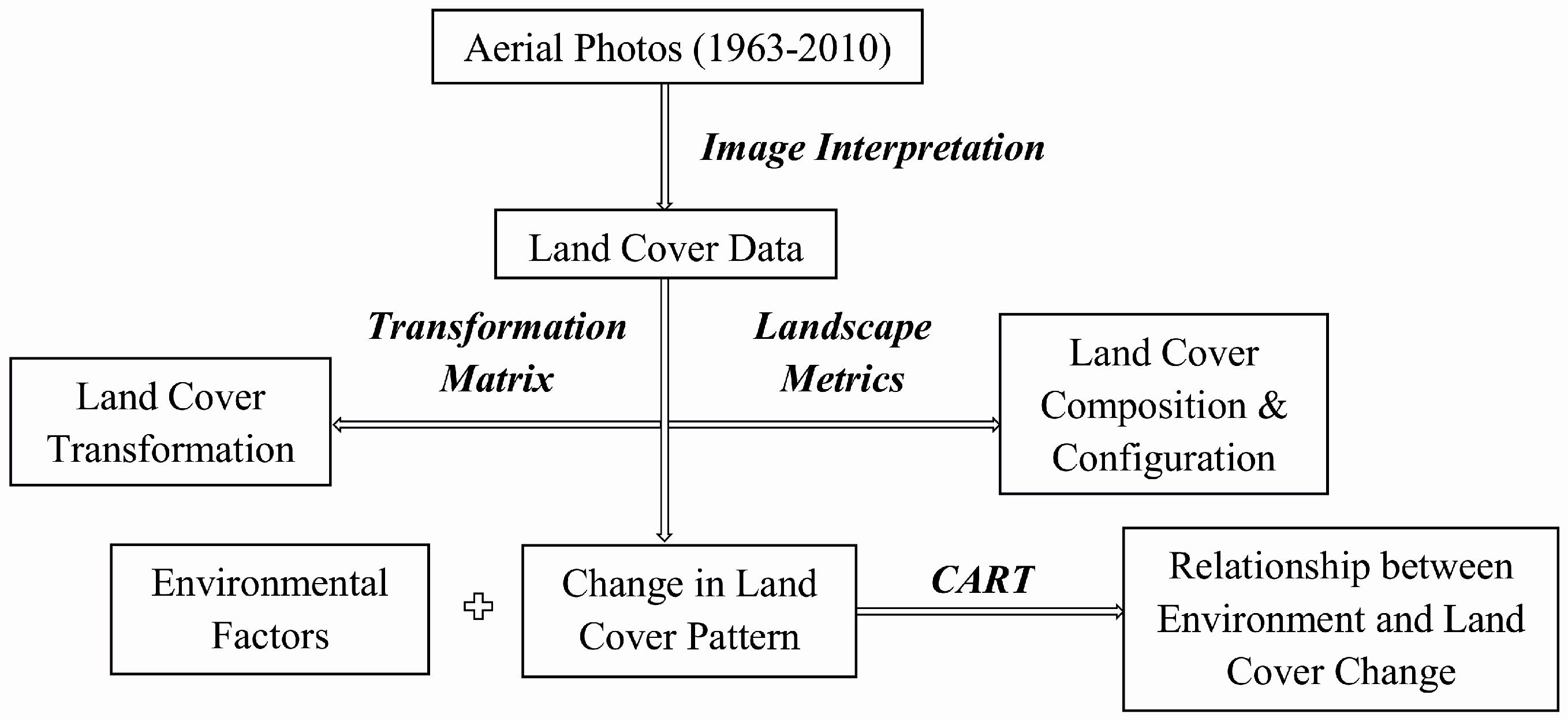
Figure 3.
Maps with changes of land cover in all study sites between 1963 and 2010. (a) Barbing; (b) Gmünd; (c) Irlbach; (d) Niederalteich; (e) Langkünzing. Abbreviation of change types please see Table A1.
Figure 3.
Maps with changes of land cover in all study sites between 1963 and 2010. (a) Barbing; (b) Gmünd; (c) Irlbach; (d) Niederalteich; (e) Langkünzing. Abbreviation of change types please see Table A1.

Figure 4.
The CART result of riparian forest change and environmental factors from 1963 to 1978. Abbreviations: RR: stable riparian forest; R-A: riparian forest to arable land; R-G: riparian forest to grassland; R-F: riparian forest to other forests; R-E: riparian forest to other land cover; the small letters refer to the study sites, see Figure 1.

Figure 5.
The CART result of grassland change and environmental factors from 1963 to 1978. Abbreviations: GG: stable grassland; G-A: grassland to arable land; G-R: grassland to riparian forest; G-F: grassland to other forests; G-E: grassland to other land cover; S: sand; Sl & lS: loamy sand; SL: very loamy sand; sL: sandy loam; L: loam; MoL: moor/loam, soil consisting of peat and loam; the small letters refer to the study sites, see Figure 1.

Table 1.
Description of the five study sites.
| Study Site | Area (ha) | Area of Active Floodplain (ha) | Mean Elevation (m a.s.l.) | Mean Slope (°) | Mean Soil Rating Index * |
|---|---|---|---|---|---|
| Barbing | 425 | 203 | 329 | 1.0 | 47.3 |
| Gmünd | 422 | 198 | 331 | 1.6 | 53.1 |
| Irlbach | 423 | 41 | 319 | 1.4 | 59.3 |
| Niederalteich | 428 | 64 | 310 | 1.0 | 53.2 |
| Langkünzing | 426 | 48 | 305 | 1.0 | 53.8 |
Note: * Definition please see Section 2.3. Abbreviation: a.s.l.: above mean water level.
Table 2.
Classification of land cover into five types and 22 subtypes.
| Type | Subtype | Description |
|---|---|---|
| Woody vegetation | Riparian forest | Woodland adjacent to water bodies (e.g., the Danube River, backwater, backwater lake and creek) |
| Forest | A complex of trees and other woody vegetation not adjacent to the water body | |
| Copse | A thicket of trees or shrubs | |
| Agricultural land | Arable land | Land where crops such as maize, wheat and rye are sown |
| Grassland | Grass-dominated land mown for fodder production or grazed | |
| Orchard | Garden with fruit trees close to settlements | |
| Water body | Artificial pond | A gravel pit for extraction of gravel filled with water |
| Backwater | A water body periodically or seasonally connected to the main channel | |
| Backwater lake | A stagnant water body close to and not connected with the main channel | |
| Creek | A small narrow stream | |
| Ditch | A long narrow excavation for drainage and irrigation | |
| River | Danube River | |
| Margin | Field hedge | Closely spaced shrubs and trees in line separating fields from each other |
| Field margin | Non-woody vegetation and grass strips in line between fields | |
| Road hedge | Closely spaced shrubs and trees in line separating roads from adjoining fields or other facilities | |
| Road margin | Non-woody vegetation and grass strips in line separating road from adjoining fields or other facilities | |
| Built-up Land | Vegetated path | Unpaved path covered with vegetation (e.g., in forest, between fields) |
| Path | Paved path with concrete or other surfaces | |
| Road | Routes with one or more lanes | |
| Settlements | Houses/homesteads grouped together | |
| Construction site | Bare land used for construction | |
| Industrial land | Land used for industrial purposes (e.g., wastewater treatment) |
Table 3.
Landscape metrics calculated at landscape and class levels [56].
Table 3.
Landscape metrics calculated at landscape and class levels [56].
| Abbreviation | Metrics | Description | Unit | Scale Level |
|---|---|---|---|---|
| LSI | Landscape Shape Index | Shape complexity of patches compared to standard shape | None | Landscape & class level |
| MPS | Mean Patch Size | Average patch size of each land cover | ha | Class level |
| MESH | Effective Mesh Size | Probability that two randomly chosen points of land cover located in the same patch | ha | Landscape & class level |
| PROX_MN | Mean Proximity Index | Proximity of all patches whose edges are within a specified search radius of the focal patch (in this study the radius is defined as 500 m) | None | Class level |
| SHDI | Shannon’s Diversity Index | Diversity of land cover patches based on the number and distribution of patches | None | Landscape level |
| SHEI | Shannon’s Evenness Index | Evenness of land cover patches based on the number and distribution of patches | None | Landscape level |
Table 4.
Net change of land cover in floodplain parts during all periods.
| Land Cover Type | Active Floodplain | Former Floodplain | ||||
|---|---|---|---|---|---|---|
| 1963–1978 | 1978–1995 | 1995–2010 | 1963–1978 | 1978–1995 | 1995–2010 | |
| Riparian forest | 4.01% | 3.14% | −2.34% | 0.07% | 0.07% | 0.48% |
| Forest | 0.21% | 0.03% | 2.63% | 0.00% | 0.07% | 0.67% |
| Copse | 0.44% | −0.09% | 0.11% | 0.68% | 1.02% | −0.41% |
| Arable land | −6.20% | −2.18% | −2.89% | 0.92% | −1.42% | −0.50% |
| Grassland | −2.11% | −1.90% | −1.05% | −4.29% | −1.50% | −0.92% |
| Orchard | −0.06% | 0.04% | −0.01% | −0.15% | −0.07% | 0.13% |
| Artificial pond | −0.02% | 0.02% | 0.04% | 0.85% | 1.51% | 0.42% |
| Backwater | 4.00% | −0.46% | 3.24% | 0.04% | −0.01% | 0.04% |
| Backwater lake | −0.45% | 0.31% | 0.16% | 0.00% | 0.03% | 0.01% |
| Creek & Ditch | −0.03% | 0.26% | −0.16% | 0.00% | −0.05% | −0.02% |
| Field hedge/margin | 0.31% | −0.16% | −0.09% | 0.51% | −0.28% | 0.05% |
| Road hedge/margin | −0.04% | 0.74% | 0.07% | 0.56% | 0.12% | 0.05% |
| Vegetated path | 0.01% | −0.38% | −0.01% | 0.04% | 0.13% | −0.39% |
| Path | 0.14% | 0.39% | −0.05% | 0.22% | 0.00% | 0.16% |
| Road | 0.01% | 0.22% | −0.15% | 0.48% | 0.04% | 0.03% |
| Settlements | 0.01% | 0.04% | 0.08% | 0.28% | 0.20% | 0.32% |
| Construction site * | −0.23% | 0.10% | −0.14% | |||
Note: * construction site only exists in the former floodplain.
Table 5.
Transformation matrix between land cover from 1963 to 2010.
| Floodplain Type | 1963–1978 | 1978–1995 | 1995–2010 | |||
|---|---|---|---|---|---|---|
| Land Cover Change | Changed Area (%) | Land Cover Change | Changed Area (%) | Land Cover Change | Changed Area (%) | |
| Active Floodplain | A-G | 6.0 | A-G | 5.4 | A-G | 4.0 |
| G-A | 3.4 | G-A | 4.8 | G-A | 1.4 | |
| G-R | 3.2 | G-R | 2.4 | G-F | 1.5 | |
| Total * | 26.7 | total | 25.2 | total | 20.1 | |
| Former Floodplain | A-G | 4.0 | A-G | 3.7 | A-G | 2.6 |
| G-A | 7.0 | G-A | 4.0 | G-A | 2.8 | |
| total | 22.1 | total | 20.1 | total | 14.7 | |
Note: A-G: Arable land to grassland; G-A: grassland to arable land; G-R: grassland to riparian forest; G-F: grassland to other forests. * The total change percentage is not the sum of the values in the table, but it also includes those changes lower than 1%, which are not shown here.
Table 6.
Mean values of structural metrics: landscape, arable land, grassland and riparian forest in active and former floodplains from 1963 to 2010.
Table 6.
Mean values of structural metrics: landscape, arable land, grassland and riparian forest in active and former floodplains from 1963 to 2010.
| Landscape Metrics | Active Floodplain | Former Floodplain | ||||||
|---|---|---|---|---|---|---|---|---|
| 1963 | 1978 | 1995 | 2010 | 1963 | 1978 | 1995 | 2010 | |
| Landscape | ||||||||
| LSI | 11.06 ± 0.80 | 10.62 ± 1.01 | 10.84 ± 1.22 | 9.96 ± 1.34 | 11.45 ± 2.24 | 12.05 ± 2.27 | 12.91 ± 1.63 | 12.48 ± 1.57 |
| MESH (ha) | 20.14 ± 7.17 | 18.88 ± 6.69 | 13.70 ± 2.27 | 18.50 ± 2.52 | 33.68 ± 10.68 | 30.76 ± 11.55 | 28.48 ± 14.16 | 26.93 ± 11.16 |
| SHDI ** | 1.26 ± 0.09 | 1.33 ± 0.08 | 1.29 ± 0.11 | 1.30 ± 0.13 | 0.95 ± 0.02 | 0.98 ± 0.06 | 1.15 ± 0.08 | 1.17 ± 0.12 |
| SHEI *** | 0.51 ± 0.04 | 0.53 ± 0.03 | 0.51 ± 0.02 | 0.54 ± 0.04 | 0.37 ± 0.02 | 0.37 ± 0.02 | 0.42 ± 0.03 | 0.43 ± 0.04 |
| Riparian forest | ||||||||
| LSI *** | 10.4 ± 1.65 | 11.04 ± 1.50 | 10.92 ± 1.60 | 10.12 ± 1.81 | 3.40 ± 1.53 | 3.67 ± 1.50 | 5.51 ± 1.58 | 4.54 ± 1.36 |
| MPS (ha) *** | 1.21 ± 0.14 | 1.91 ± 0.35 | 2.21 ± 0.51 | 1.92 ± 0.27 | 0.13 ± 0.08 | 0.37 ± 0.16 | 0.29 ± 0.11 | 0.38 ± 0.23 |
| MESH (ha) *** | 1.38 ± 0.72 | 2.76 ± 1.52 | 3.40 ± 1.57 | 4.38 ± 3.04 | 0.004 ± 0.004 | 0.005 ± 0.003 | 0.008 ± 0.003 | 0.018 ± 0.013 |
| PROX_MN *** | 92.76 ± 28.17 | 192.92 ± 61.95 | 475.44 ± 184.33 | 131.04 ± 35.44 | 4.02 ± 2.57 | 3.84 ± 3.38 | 12.61 ± 5.13 | 1.78 ± 2.86 |
| Grassland | ||||||||
| LSI | 10.16 ± 1.04 | 8.37 ± 0.93 | 8.76 ± 1.28 | 7.84 ± 0.92 | 10.24 ± 2.29 | 9.40 ± 1.76 | 8.95 ± 1.45 | 8.34 ± 1.48 |
| MPS (ha) * | 0.61 ± 0.08 | 0.63 ± 0.16 | 0.66 ± 0.09 | 0.87 ± 0.12 | 0.48 ± 0.04 | 0.50 ± 0.06 | 0.53 ± 0.15 | 0.50 ± 0.14 |
| MESH (ha) * | 4.71 ± 2.51 | 3.70 ± 2.06 | 3.98 ± 2.88 | 4.82 ± 2.95 | 1.10 ± 0.37 | 0.60 ± 0.32 | 0.55 ± 0.33 | 0.53 ± 0.37 |
| PROX_MN | 260.80 ± 135.28 | 190.80 ± 81.88 | 140.19 ± 54.21 | 146.77 ± 86.10 | 143.39 ± 51.05 | 59.90 ± 20.29 | 68.57 ± 35.09 | 54.17 ± 28.68 |
| Arable land | ||||||||
| LSI ** | 5.61 ± 0.34 | 5.16 ± 0.65 | 4.18 ± 0.88 | 3.56 ± 0.71 | 7.83 ± 1.69 | 7.54 ± 1.59 | 7.49 ± 1.33 | 7.06 ± 1.40 |
| MPS (ha) | 0.53 ± 0.14 a | 0.55 ± 0.15 a | 1.08 ± 0.25 ab | 1.42 ± 0.33 b | 0.43 ± 0.06 a | 0.15 ± 0.07 ab | 1.19 ± 0.06 ab | 1.39 ± 0.05 b |
| MESH (ha) *** | 12.09 ± 7.92 | 10.47 ± 7.47 | 4.01 ± 1.93 | 4.73 ± 2.85 | 32.51 ± 10.96 | 29.94 ± 11.69 | 27.76 ± 14.24 | 26.18 ± 11.27 |
| PROX_MN ** | 326.47 ± 182.93 | 626.89 ± 396.60 | 312.33 ± 250.61 | 347.65 ± 304.18 | 2111.83 ± 838.54 | 2269.85 ± 896.74 | 1982.81 ± 798.20 | 2874.85 ± 1102.47 |
Note: Mean ± SE; Abbreviations: LSI = landscape shape index; MPS = mean patch size; MESH = effective mesh size; PROX_MN = mean proximity index; SHDI = Shannon’s diversity index; SHEI = Shannon’s evenness index. Signif. Codes within factor “floodplain type”: 0 ‘***’ 0.001 ‘**’ 0.01 ‘*’ 0.05 ‘.’ 0.1 ‘ ’ 1. Letters “a” “b” “ab”: significant groups (p < 0.1) within factor “Year”.
Table 7.
The relative importance of environmental factors to land cover change.
| Environmental Factors | Arable Land Change | Grassland Change | Riparian Forest Change | ||||||
|---|---|---|---|---|---|---|---|---|---|
| 1963–1978 | 1978–1995 | 1995–2010 | 1963–1978 | 1978–1995 | 1995–2010 | 1963–1978 | 1978–1995 | 1995–2010 | |
| Aspect | 2 | 1 | 2 | 1 | 1 | 5 | 10 | 11 | 8 |
| Distance to river | 15 | 14 | 22 | 4 | 13 | 31 | 43 | 7 | 26 |
| Height above MW | 10 | 22 | 22 | 18 | 21 | 18 | 20 | 46 | 26 |
| Slope | 4 | 4 | 4 | 2 | 2 | 5 | 9 | 2 | 5 |
| Soil rating index | 42 | 18 | 16 | 18 | 13 | 26 | |||
| Soil texture | 7 | 18 | 16 | 26 | 9 | 10 | |||
| Study site | 20 | 23 | 18 | 31 | 41 | 6 | 17 | 34 | 34 |
Note: Results were calculated with CART, and the relative importance to each land cover change type during one period sums up to 100.
© 2017 by the authors. Licensee MDPI, Basel, Switzerland. This article is an open access article distributed under the terms and conditions of the Creative Commons Attribution (CC BY) license (http://creativecommons.org/licenses/by/4.0/).
Share and Cite
MDPI and ACS Style
Xu, F.; Otte, A.; Ludewig, K.; Donath, T.W.; Harvolk-Schöning, S. Land Cover Changes (1963–2010) and Their Environmental Factors in the Upper Danube Floodplain. Sustainability 2017, 9, 943. https://doi.org/10.3390/su9060943
AMA Style
Xu F, Otte A, Ludewig K, Donath TW, Harvolk-Schöning S. Land Cover Changes (1963–2010) and Their Environmental Factors in the Upper Danube Floodplain. Sustainability. 2017; 9(6):943. https://doi.org/10.3390/su9060943
Chicago/Turabian StyleXu, Fang, Annette Otte, Kristin Ludewig, Tobias W. Donath, and Sarah Harvolk-Schöning. 2017. "Land Cover Changes (1963–2010) and Their Environmental Factors in the Upper Danube Floodplain" Sustainability 9, no. 6: 943. https://doi.org/10.3390/su9060943
Note that from the first issue of 2016, this journal uses article numbers instead of page numbers. See further details here.