Development of a GIS Tool for High Precision PV Degradation Monitoring and Supervision: Feasibility Analysis in Large and Small PV Plants

Abstract

It is well known that working photovoltaic (PV) plants show several maintenance needs due to wiring and module degradation, mismatches, dust, and PV cell defects and faults. There are a wide range of theoretical studies as well as some laboratory tests that show how these circumstances may affect the PV production. Thus, it is mandatory to evaluate the whole PV plant performance and, then, its payback time, profitability, and environmental impact or carbon footprint. However, very few studies include a systematic procedure to quantify and supervise the real degradation effects and fault impacts on the field. In this paper, the authors first conducted a brief review of the most frequent PV faults and the degradation that can be found under real conditions of operation of PV plants. Then, they proposed and developed an innovative Geographic Information System (GIS) application to locate and supervise them. The designed tool was applied to both a large PV plant of 108 kWp and a small PV plant of 9 kWp installed on a home rooftop. For the large PV plant, 24 strings of PV modules were modelized and introduced into the GIS application and every module in the power plant was studied including voltage, current, power, series and parallel resistances, fill factor, normalized PV curve to standard test conditions (STC), thermography and visual analysis. For the small PV installation three strings of PV panels were studied identically. It must be noted that PV modules in this case included power optimizers. The precision of the study enabled the researchers to locate and supervise up to a third part of every PV cell in the system, which can be adequately georeferenced. The developed tool allows both the researchers and the investors to increase control of the PV plant performance, to lead to better planning of maintenance actuations, and to evaluate several PV module replacement strategies in a preventive maintenance program. The PV faults found include hot spots, snail tracks, ethylene vinyl acetate (EVA) discoloration, PV cell fractures, busbar discoloration, bubbles and Si discoloration.

1. Introduction

The operation and maintenance of a photovoltaic (PV) power plant is of extreme importance to guarantee its optimal performance. In fact, monitoring is not just a regular recording of data but involves a more detailed analysis in order to prevent possible malfunctions with its associated power and economic losses. However, most photovoltaic power plants record few operative data for proper operation, but it is not usual that the maintenance service carries out a detailed analysis. Effective maintenance involves at least semiautomatic analysis and alerts. In this way, the maintenance operator is allowed to make immediate decisions and solve safety problems and minimize power losses [1].

The main objective of this study is to design a tool that allows the maintenance service to carry out an effective supervision of the power plant and, more importantly, to monitor the evolution of the modules behavior in an easy and feasible way. In fact, automated monitoring of photovoltaic plants is becoming necessary to evaluate the aging of the panels and the early detection of operating failures. Thus, significantly more effective management plans, preventive maintenance policies, and early replacement of poor performance components can be carried out with successful results.

Accurate measurement, control and evaluation systems are fundamental for the main participant agents in the photovoltaic industry. For device manufacturers, the evaluation of the performance of their products is a reference of their quality manufacturing processes. On the other hand, researchers from companies can take advantage of them and use that information to identify future needs in the industry and test real working conditions. For PV plant promoters and owners, realistic performance data are essential for investment decision making.

The related literature shows several strategies based on physical modelling and polynomial regression between DC power estimations and real AC power production. Subsequently, these results are applied to the detection of real and/or potential failures in the PV field [2]. However, these sort of techniques are consequently found to be limited in the sense they do not detect the existing anomaly (e.g., module failure, power production losses, safety dangers, etc.) until it occurs and the consequences cannot be avoided. Furthermore, these techniques are not adequate to implement effective preventive maintenance strategies or carry out an effective and economic component replacement schedule.

Other monitoring approaches are based on performance indicators calculated through electro-thermal modelling techniques of the PV plant [3]. As these indicators are calculated on a daily basis, they are also not effective for our purposes.

On the other hand, the latest data acquisition systems that have been integrated on the supervision and monitoring devices for photovoltaic plants are based on wireless technology such as Zigbee, according to IEEE 802.15.4, based specification for personal area networks. Parameters such as temperature, irradiation, DC power input in the inverter, and AC power output to the grid can be easily obtained. Furthermore, the acquired data can be uploaded to the cloud almost in real time and notification alerts sent to the power plant owners and maintenance service [4]. However, these systems still do not integrate georeferencing tools that may help to improve the application of a preventive maintenance strategy.

Our experience both in the laboratory and in the real field regarding PV power plants have led us to design a new methodology to locate and analyze malfunctions, faults, and outrageous performances from the plant components in a global context. The analysis is carried out in a laboratory with results of high interest, but often they do not result operatively in the application of real maintenance plans. Although test conditions in the laboratory allow a deep analysis of the PV components under study, it involves unaffordable costs for the owners and sometimes requires the complete or part shutdown of the installation. Moreover, test conditions in the laboratory may not be representative of the real working conditions in the working field. Thus, the conclusions from the laboratory test may be decontextualized. On the other hand, analysis techniques in the field are influenced by climatic and environmental conditions, that are not usually stable. Thus carrying out a systematic procedure becomes more difficult.

For this reason, a new methodology has been proposed combining the precision of standard laboratory tests and a feasible and effective maintenance procedure. The integration of Geographic Information System (GIS) platforms supposes a significant advantage in the sense that all test related information is adequately organized and georeferenced. Thus, not only can the particular impacts of a defect on a single component be studied, but its impact on the overall performance can then be analyzed. Then, predictive techniques that analyze variations on the behavior of apparently sane components can be applied and possible malfunctions on a certain zone of the power plant predicted.

A properly developed GIS tool allows a comprehensive analysis of the territory with application to any activity that involves a spatial component. In this way, GIS technology has a wide field of application in the management of resources. In addition, this is an essential tool in decision-making tasks where the spatial component has a certain relevance.

In the past decade several applications of GIS tools to the Energy field have arisen, specifically to locate energy resources, to build a solar atlas, etc. As an example, Höhn et al. applied a GIS tool to analyze the spatial distribution of biomass resources in a certain region of Finland to optimize the location of biogas power plants [5]. On the other hand, other authors have taken advantage of GIS tools to create a solar atlas and estimate with high precision the power potential of Concentrated Solar Energy (CSP) power plants [6].

Also in the field of photovoltaic energy, the application of GIS techniques is an innovative approach that has quickly taken relevance, especially in the design, management, and supervision of large PV power plants. Thus, just to cite some examples, Kakumoto et al. present a GIS based technique to estimate PV production taken into account with precision the shadowing effect [7]; and Tsanakas et al., by the combination of aerial triangulation techniques and terrestrial georeferencing, propose a technique to create virtual dynamic maps of a power plant, including georeferenced thermal images [8]. Other authors have used GIS together with Global Positioning Systems (GPS) and Unmanned Aerial Vehicles (UAV) to propose an efficient inspection and maintenance of PV power plants [9].

According to these examples, the potential of the utilization of GIS based methodologies in the energy field seems to be of great interest in the near future.

The purpose of this work is to extend the application of the GIS tools in the photovoltaic field, not only to the resource location, but in the operation and maintenance of PV power plants as well. This is really of interest in large plants. Early fault detection may result in a significant improvement of the power plant performance, and the inclusion of spatial information is a novel approach that may lead to new predictive and preventive maintenance programs.

This study aims to evaluate the potential of a specifically designed GIS tool in the location of PV faults and analysis of the degradation effects on PV power plants working in real operating conditions. As a case study, the proposed tool was applied to two representative PV plants: a 108 kW peak power (kWp) grid connected power plant and a 9 kWp self-consumption power plant.

The most commonly spread real degradation effects and fault impacts on the field, observable or measurable, that affect or may affect the future production of energy of the photovoltaic plants are included in the analysis. Only the faults on the PV modules are included. Wiring degradation, inverter faults, aging and other electrical and mechanical malfunctions are excluded from the preliminary version of the developed tool, although they may be included in future versions.

This article is organized in five sections. First, a brief review of the most common PV faults is displayed. Then, the methodology and the tool characteristics are described. In Section 4, the application of the developed tool is presented and two representative case studies are fully described including the results discussion of the developed GIS tool implementation. Finally, the last section includes the main conclusions and future research directions.

2. State of the Art of PV Module Defects

The literature defines a failure in a photovoltaic module as an effect that degrades the module power output which is not reversed by normal operation, or that creates a safety issue. Sometimes, both effects can occur simultaneously. A purely aesthetic problem is, then, not considered as a failure of the PV module. Wiring and module degradation, mismatches, dust and PV cell defects and faults, are considered as failures of PV modules [10].

A systematic review has been conducted in order to show the state of the art in this field with precision. According to Urra Medina et al., a systematic review is defined as a process to identify the core of a narrative review which may result in value of interest in practice [11]. In this case, the identification of the review purpose answers the question “which PV faults are the most representative in the literature and may affect more significantly the power production of a PV plant?” This research question, as required in the systematic review methodology, is delimiting, accessible and distinguishable in the literature [12]. Thus, the following fixed conditions for the review are applied:

• Sources: only papers from indexed international journals, scientific books edited by international editors, international conference proceedings, technical review reports from prestigious international organizations and open access Ph.D. Theses have been included in the research.
• Language: English and Spanish.
• Publication period: only research works published in the period from 2000 to 2016 have been considered.
• Requirements: selected contributions must be open access or available in international databases, peer-reviewed, and guaranteeing traceability in the research.
• Type: both original research contributions and review works have been included in the analysis.

Once the searching criteria were defined, the literature review was conducted and results can be seen in

Table 1. Systematic review on photovoltaic (PV) defects results. Number of references.

Failures	Conference Papers	Journal Articles	Articles in Press	Reviews and Reports	Books and Ph.D. Theses
Delamination	58	37	2	2	2
Adhesion loss from the backsheet films	4	65	0	2	11
Faults in the junction box	1	249	0	9	145
Frame breakages	2	228	0	9	122
EVA discoloration	9	28	1		4
Bubbles formation	3	237	0	10	89
Cell cracks	9	357	0	27	221
Snail tracks	6	34	0	2	13
Burn marks	0	473	0	21	264
Potential induced degradation	173	953	0	38	67
Disconnected cells and string interconnected ribbons	3	29	0	0	41
Defective by-pass diode	1	197	0	4	82
Hot spots on cells	11	636	2	34	294
TOTAL	280	3523	5	158	1355

, where the most common defects have been identified and classified. It must be noted that books and Ph.D. Theses have been grouped, as well as review works and technical reports. Results show 5321 references, where 66% are journal articles and 25% are books and Ph.D. Theses.

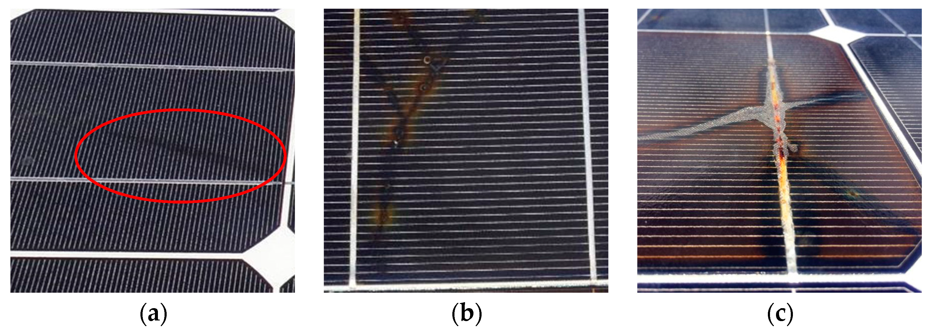
Figure 1 shows examples of several of the described defects. The following subsections describe briefly all found PV module potential failures.

2.1. Delamination

The adhesion between the glass, encapsulation, active layers and the back layers can be compromised for various reasons. Larger thin film modules and some other types of technology may also contain a transparent conductive oxide (TCO) layer from the soda-lime glass substrate. This layer may lose adhesion with the adjacent glass layer [13]. Usually, if adherence is compromised due to contamination (e.g., by inadequate cleaning of the glass) or environmental factors, delamination will occur, followed by moisture formation and, thus, corrosion. The delamination of the interfaces that are within the optical path of the light, will give rise to reflection and consequent loss of current (power) on the modules.

Delamination can be relatively easy to detect by visual inspection. The detachment of the layers can be quantified using a reflectometer. On the other hand, there are delaminations that cannot be visually identified and therefore, other methods must be used, such as pulsed active thermography or “lock-in” thermography. X-ray tomography and the ultrasound scanner are used to examine smaller delaminations. This way, a much higher resolution can be obtained, but both methods require a longer evaluation time [14].

2.2. Adhesion Loss of the Backsheet Films

Most backsheet films for PV modules are multilayer composites comprising three or more polymer layers. The outer layers have to be resistant against various weathering impact factors (e.g., irradiance, humidity etc.) Often used protection layers are fluoropolymers, such as polyvinylfluoride (PVF), polyamide (PA) or polyethylene terephthalate (PET) [15].

Reported failures of backsheets are delamination within the multilayer laminate, embrittlement leading to cracks or yellowing. The worst failures within backsheets are cracks and delaminations, as they allow enhanced water vapor and oxygen ingress into the PV module and can cause safety problems due to the loss of the isolation properties [16]. Water vapor is known to have a critical impact on various degradation phenomena like corrosion of the metallic parts, potential induced degradation (PID) of PV modules, and encapsulated decomposition. Therefore, these failure modes can reduce the performance of a PV module and shorten its lifespan. However, the yellowing effect, is reported to have no influence on the electrical performance of the modules.

2.3. Mechanical Breakage and Junction Box Faults

Mechanical breakages are usually identified as frame cracks produced due to poor handling conditions or extreme snow loads in winter.

The junction box is the container, attached to the back of the module, which protects the connection of the strings of the module to the external terminals. Usually, the junction box contains bypass diodes, which protect the cells of a series in case hot spots are produced, mainly due to partial shadowing of the module [10]. It has been reported in the field that faults in the adhesive system and overtures on the junction box provoke moisture formation and, then, wiring degradation. This type of failures affects mainly the safety, being able to produce an electric arc and, even, risk of fire.

2.4. Encapsulation Discoloration and Bubbles Formation

The encapsulation material (usually, ethylene vinyl acetate or EVA) degradation is an aesthetic issue that usually does not affect the module’s performance. However, this degradation may result in a current loss with an average of 0.5%/year and a median of 0.8%/year for a Si PV module [17].

On the other hand, bubbles are generally caused by the evolution of gas elements directly or indirectly during melt and solidification procedures, because, in the manufacturing process the photovoltaic module is exposed to inappropriate temperatures, or excessively long periods during the lamination process [18].

2.5. Cell Cracks

PV cells are made of silicon so they are very brittle. Cell cracks are formed in different lengths and orientations in the substrate of the photovoltaic cells and, often, cannot be easily seen. Cell cracks can be caused during cell production or after production. The major sources of cell cracks are packaging, transportation, reloading of PV modules, and the installation process in the field.

Once cell cracks are present in a solar module, there is an increased risk that, during the operation of the solar module, short cell cracks can develop into longer and wider cracks. This is because of mechanical stress [19] caused by wind or snow load and thermo-mechanical stress [20] on the solar modules due to temperature variations caused by passing clouds and variations in weather.

Therefore, an inactive cell area of more than 8% is not acceptable. Besides the risk of power loss there is a chance of hot spots due to inactive cell parts greater than 8%. This happens if the cracked cell has a localized reverse current path in the still active cell part. Due to the missing cell area the cell is driven into reverse bias and the full current can flow along the localized path. This may cause hot spots and therewith burn marks [21].

2.6. Snail Tracks

Snail tracks are discolorations of the silver fingers on solar cells. In the PV module the effect looks like a snail track on the front glass of the module. The discoloration occurs at the edge of the solar cell and on not visible cell cracks. The discoloration typically occurs between 3 months to 1 year after installation of the PV modules [22]. The initial discoloration speed depends on the season and the environmental conditions. During the summer and in hot climates, snail tracks seem to spread faster [10]. In [23], the authors compare the results of the PV modules affected by the snail track with a reference module under laboratory conditions. The results showed that the maximum power under standard conditions is reduced by 40%, and the energy production measured over 30 days was approximately 25% lower than expected.

2.7. Burn Marks and Hot Spots

One of the most common and typical failures in silicon modules are burn marks. This failure is associated with parts of the module that become very hot because of solder bond failure, ribbon breakage, localized heating from application of reverse current flow or other hot spots [10]. Burn marks produce unquantified power losses and safety problems.

A hot spot is a phenomenon that defines a region located in a photovoltaic module whose operating temperature is very high compared to the surrounding regions. This can happen when a cell generates less current than the rest of the cells connected in series as a consequence of the following [24]:

• Partial shading.
• Potential-induced polarization with respect to ground in modules manufactured with novel techniques (voltage, both positive and negative, depending on the type of cell considered).
• Intrinsic defects in the cell.
• Dispersion of characteristics between modules of a generator and between cells of the same module connected in series.
• Interconnection failure.

As a result, the defective cell is polarized, (the voltage between the positive and negative terminals becomes negative), and behaves as a charge dissipating in heat the power generated by the rest of the series of cells.

2.8. Potential Induced Degradation

The potential induced degradation causes power losses due to the presence of eddy currents in the PV modules. Its potential effect can reduce the power of the equipment [25].

The reported main cause of these currents is the presence of voltages gaps between the module and the ground. In most photovoltaic systems without a grounding system, the modules have a non-zero voltage that provokes this effect. Negative voltages are more frequently reported, especially under high voltage conditions, high ambient humidity and/or high ambient temperatures [26].

2.9. Disconnected Cells and String Interconnected Ribbons

Cell strings are disconnected due to the weakness of the string interconnected ribbons. The main causes of this effect are poor quality welds in the PV module production process, weak connections between the cells ribbon and the string or deep deformations. Moreover, a narrow distance between the cells promotes the cell interconnected ribbon breakage [10].

Likewise, there may be multiple consequences: shunt by cell interconnected ribbon with reduction of open circuit voltage, and broken cell interconnected ribbon with reduction of maximum power point current [27].

2.10. Defective By-Pass Diode

By-pass diodes are used to minimize the effects of partial shading on the PV module power generation. By-pass diodes are required to limit the potential of a reverse voltage produced because of partial shading [10].

Without by-pass diodes, partial shading on photovoltaic solar cells reduce dramatically their power output and can cause local overheating leading to severe damage [28].

3. Materials and Methods

In this section, the innovative developed GIS tool will be described first. Then, the measurement process and used equipment will be detailed. All measurements have been taken according to the adequate standards with the minimum uncertainties affordable using on field working equipment.

3.1. GIS Tool Implementation

A GIS is a set of programs and computer applications that allow the management of data organized in databases, referenced spatially and visualized through maps [29]. Thus, it is a powerful analysis tool that can include spatial and/or geographical data—referenced to a map—although it can also include non-spatial data.

The proposed tool in this study aimed to collect and compile a dataset of several PV power generation variable values into a GIS tool in order to easily visualize and locate problems in a PV power plant and to predict their spread. Thus, a base map and an associated database were created, as well as the proper procedures to systemize the data introduction and analysis. In this way, the study of the evolution of existing defects, including electrical and thermal parameters, becomes simpler. Moreover, as a novel approach, the developed tool allows the correlation of the PV defects existence not only with power losses on the affected PV module, but also to the overall performance of the PV power plant.

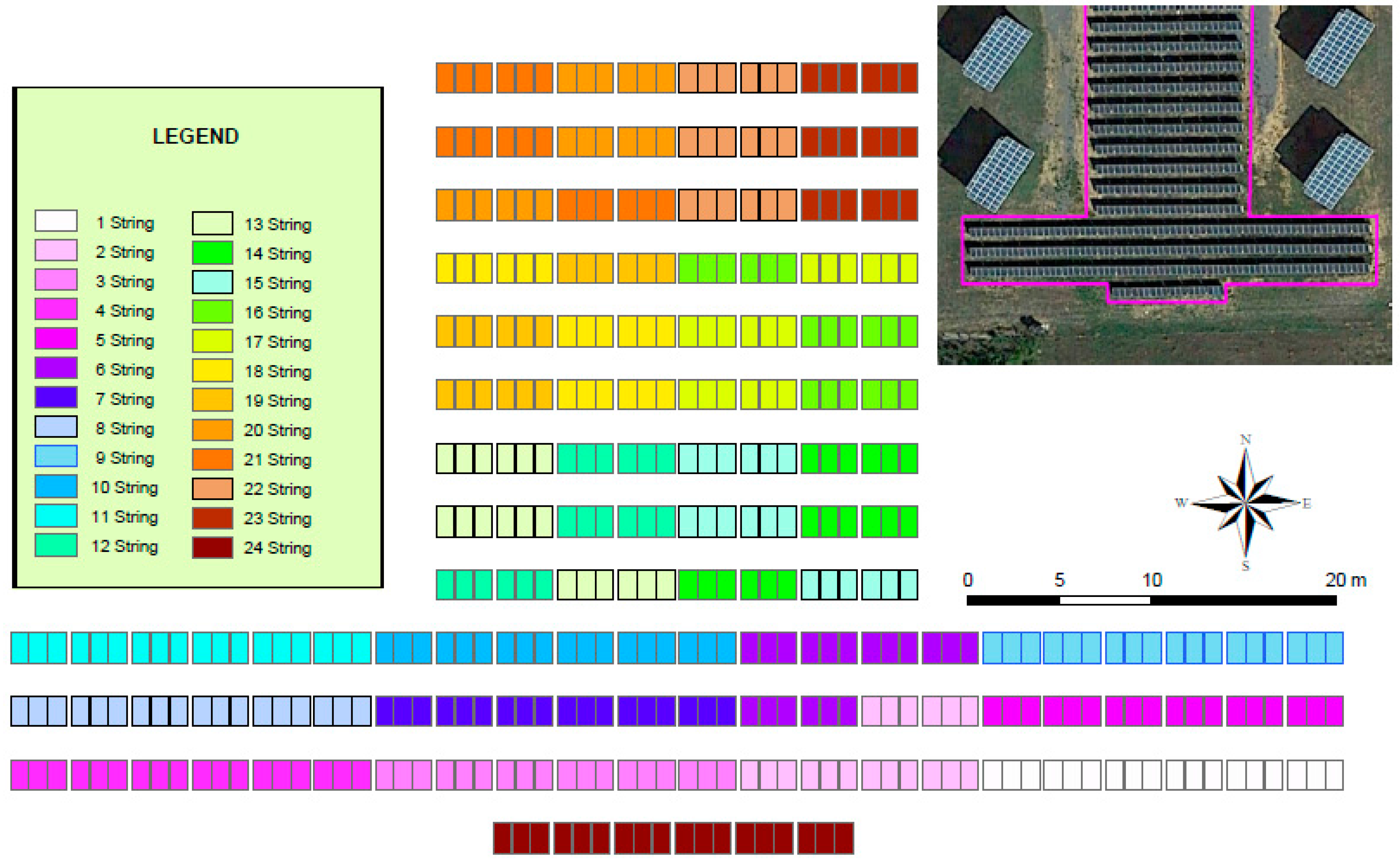
The complete PV power plant was first introduced into the GIS software (ESRI ArcGIS) by aerial ortophotographs and projected geometrical parameters. Thus, the limits of the plots and the geographical position of the PV series strings organization were set. Figure 2 shows both the representation of the analyzed PV plant and the division into strings.

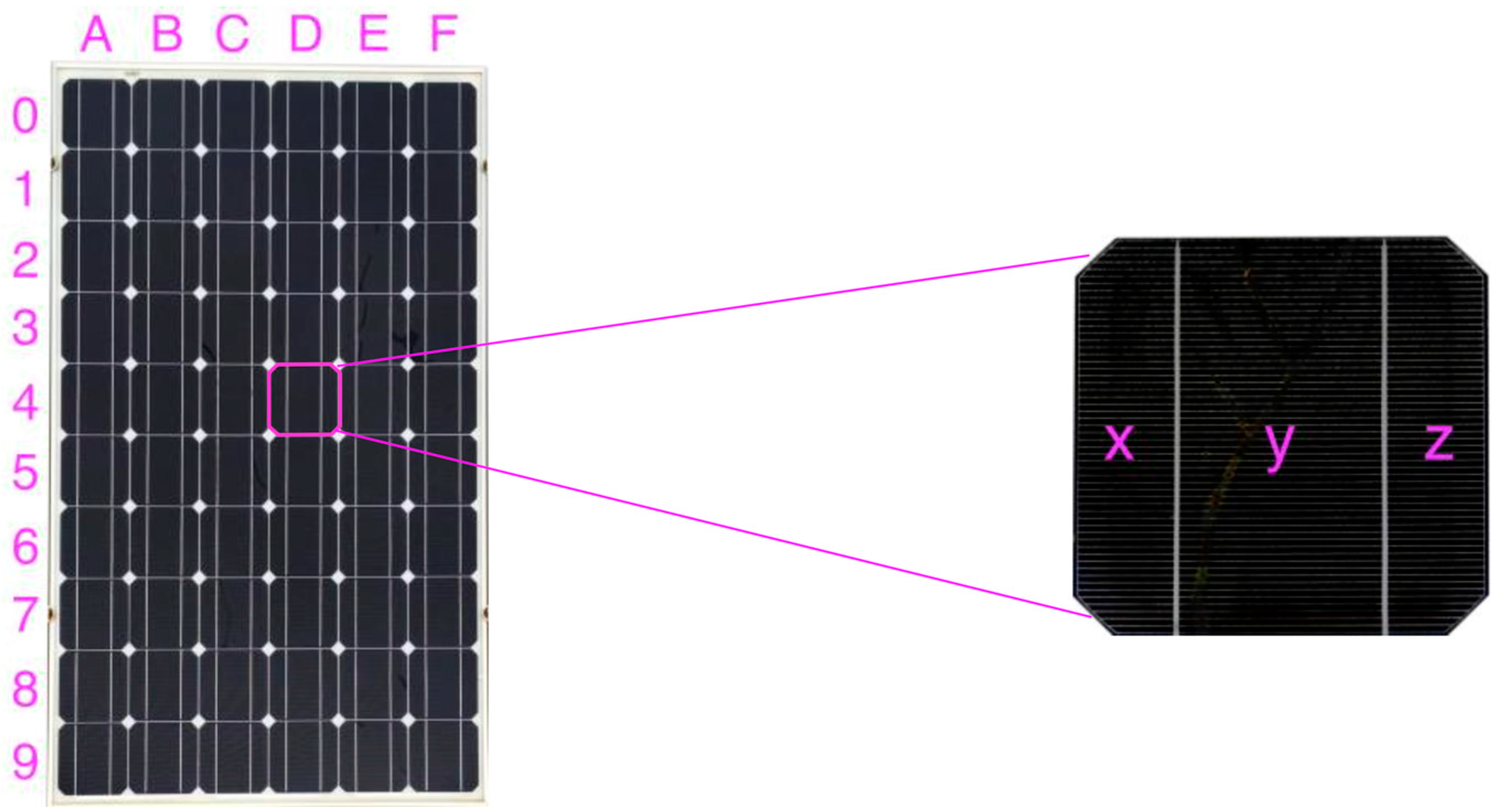
Furthermore, it is mandatory to identify the exact position within the panel of the possible faults. For this reason, the split installation with photovoltaic panels was taken into account and the thirds of cell within each panel. This means that the 60 solar cells of each panel are divided into three parts, thus each photovoltaic module is formed by 180 thirds of cells. The maps were georeferenced by assigning them projected coordinates ETRS89 UTM 30N.

As seen in Figure 2, the reference of the position of the modules within the string series begins in the bottom left hand corner of the map. Then, each PV module, in addition to being identified with the rack number, can also be identified with a simple code which includes the series string and the relative position within the string series.

A systematic procedure must be established to identify the geographical position of the defect within the panel. As each photovoltaic module consists of 180 thirds of cells, the following nomenclature was proposed. Each cell in the solar panel is divided into 10 rows (0–9) and 6 columns (A–F). In turn, each cell has been divided into 3 thirds (X, Y or Z), depending on their position. Therefore, when indicating the position of a defect, the third of cell where it is located within the panel can be identified by a three alphanumerical symbols code (e.g., 2CY). Figure 3 shows the adopted identification system on a panel.

Once the graphical part of the GIS tool has been defined and the identification procedure for each component has been established, a georeferenced database (geodatabase) was implemented. The geodatabase is a set of several types of geographic datasets embedded in a common file system folder. In our case, a geodatabase was specifically created having a comprehensive information model to represent and manage geographic information related to a PV power plant. This comprehensive information model was implemented as a series of tables that store entity classes, raster datasets and attributes.

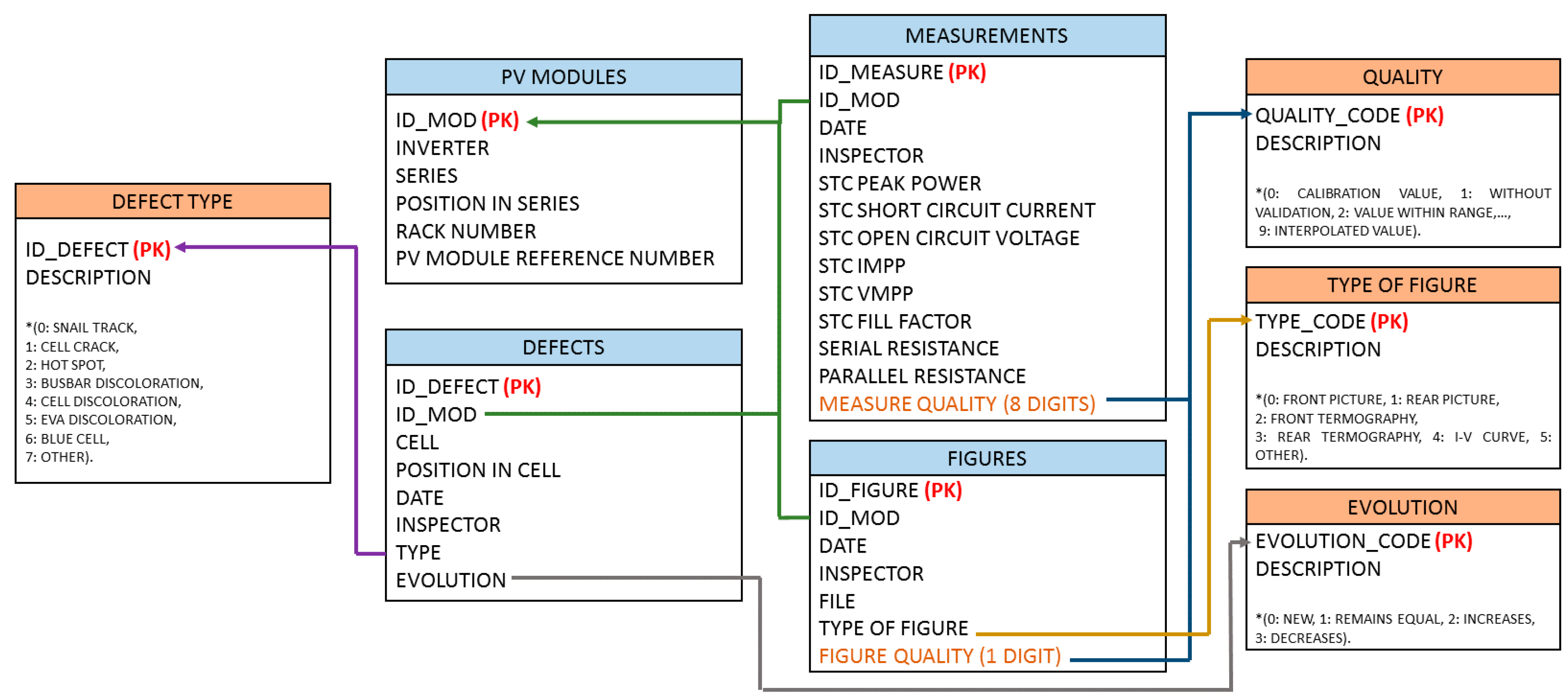
The designed information model is divided into three types of information: electrical variable measures, graphic information (pictures and thermographies), as well as defects existence and description. Figure 4 shows the scheme diagram of the relational database. According to the three types of information, it is organized into four main tables and four auxiliary tables.

The first main table, named PV MODULES, includes all the information related to the analyzed PV module, including an identifier code (ID_MOD) which is the Primary Key of the table (identifies uniquely each record), the associated inverter (INVERTER), the string series (SERIES), the relative position in the series (POSITION IN SERIES), the rack number (RACK NUMBER), and its manufacturing reference code (PV MODULE REFERENCE NUMBER).

The table named MEASUREMENTS includes all the measured electrical variables that will allow the performance analysis. It assigns to each measurement a unique identifier (ID_MEASURE) and relates each measurement record to the PV module through the ID_MOD. It also includes the date when the measurement was taken (DATE) and the inspector who did it (INSPECTOR). The factory settings were introduced into the database setting INSPECTOR as “FACTORY” and the installation date as DATE. Moreover, in order to guarantee a proper analysis, the measurement quality (metadata) was included in another parameter named MEASURE QUALITY, which is an 8 digits’ code described in the auxiliary table named QUALITY.

The quality code is a metadata field which gives information about the stored data. It is a number between 0 and 9 that can take the following values: 0: the record is a calibration value; 1: the record has no validation; 2: the record has been checked to be in range; 3: the record has passed the time coherence test (assigned timestamp is correct); 4: the record has passed the internal coherence test; 5: the record has passed the time series coherence test; 6: the record has passed the spatial coherence test; 7: the record is considered not valid because of external disturbances; 8: the measure was not recorded; 9: the measure was not directly measured (it was interpolated or calculated from others). There exists one digit for each electrical measured value.

PV defects and faults were introduced in the DEFECTS table. Each record identifies the affected module (ID_MOD), the cell through the location code (CELL), the affected third of cell (POSITION IN CELL) as well as the date (DATE), inspector (INSPECTOR), type of defect (TYPE) and evolution of the defect in the module (EVOLUTION).

Type value is an identifier described in the auxiliary table named DEFECT TYPE. PV faults were coded in the form 0: snail track; 1: cell crack; 2: hot spot; 3: busbar discoloration; 4: cell discoloration; 5: EVA discoloration; 6: blue cell and 7: other.

On the other hand, the EVOLUTION field in the DEFECTS table is associated with the auxiliary table named EVOLUTION. The evolution of the defect in the PV module is included according to the following descriptions 0: new defect or not detected before; 1: already detected but remains equal to the previous inspection; 2: has increased from the previous inspection and 3: has decreased from the previous inspection.

Finally, graphic information can also be included. In this case, front and rear pictures of each analyzed module and front and rear thermographies are taken. Moreover, the I-V curve obtained by a PV curve tracer is stored. This information is organized in the FIGURES table which includes a hyperlink to the file (FILE), the type of figure (TYPE OF FIGURE) and its quality (FIGURE QUALITY). The type of figure is related to the auxiliary table named TYPE OF FIGURE. The figure quality is especially relevant in the case of thermographies and it is a one-digit code whose description can be found in the previously described auxiliary table named QUALITY.

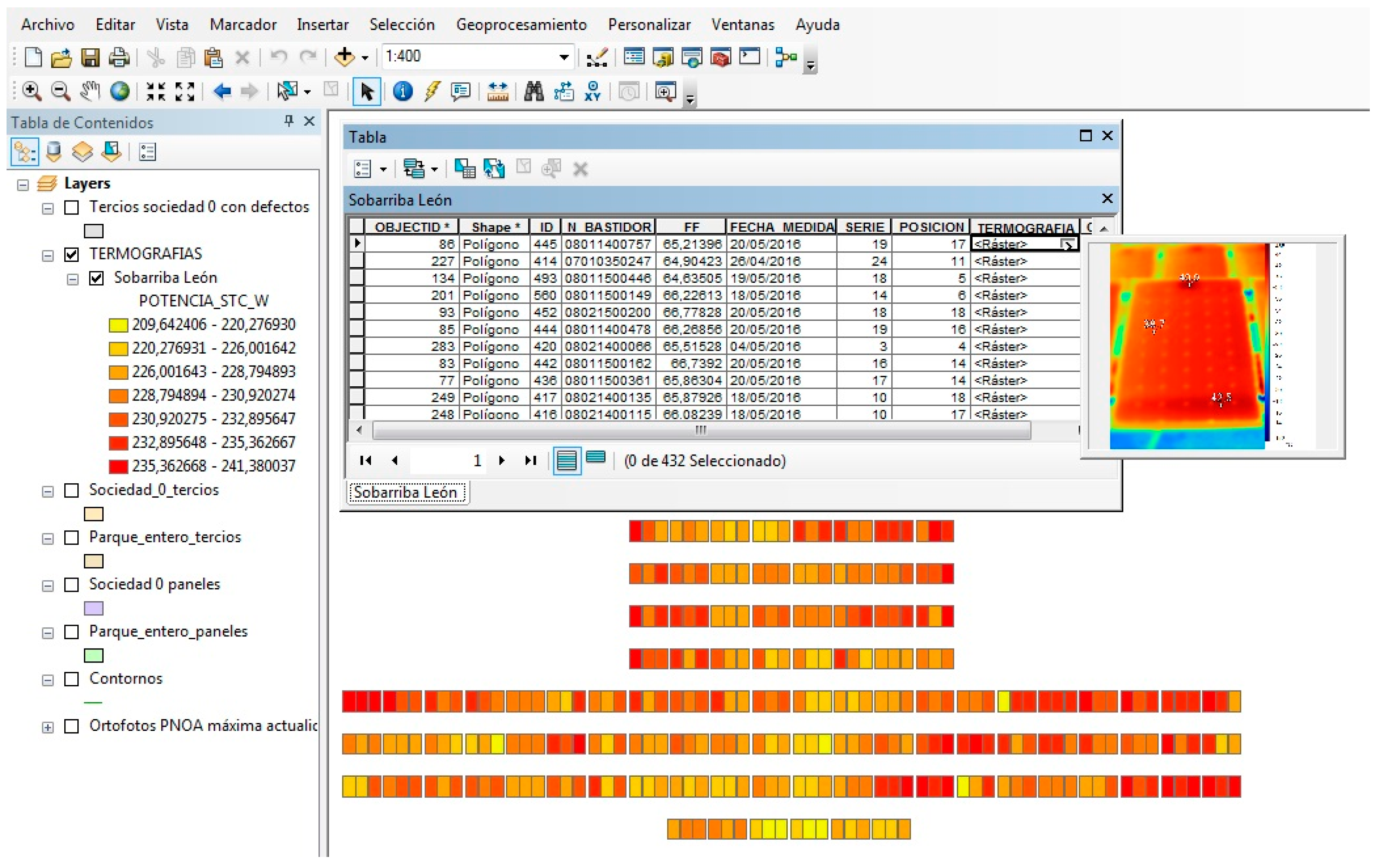
As can be seen in Figure 5, both pictures, thermographies and I-V curves are associated and spatially referenced to each of the modules. This result is very useful as it allows spatially relating the measured attributes in each panel with this graphical information. Moreover, all graphics are available not only from the geodatabase but for quick access through the GIS map.

Once the electrical measurements, faults detection, and graphical information are obtained, all data can be compiled into a complete project constituting a GIS.

3.2. Measurement Procedures and Equipment

The followed methodology for the PV power plant status monitoring includes a visual and a measurement inspection. The visual inspection includes taking pictures of the front and rear parts of the PV module, as well as both calibrated thermographies. The measurement inspection involves the characterization of the PV module performance by the measurement of its characteristic I-V curve at working conditions and its extrapolation to the standardized STC conditions (incident global irradiance of 1000 W/m², cell temperature of 25 °C and 1.5 air mass).

For the analysis of the thermal distribution in the PV modules a Fluke Ti40 thermal camera was used. It is mandatory to guarantee that there are no shadows on the PV modules during the process. This could cause unexpected irregular thermal areas conducting to a misinterpretation of the results. Moreover, high wind speed conditions must be avoided as convection thermal exchange may diffuse the thermal image.

The most favorable conditions to take a good quality and representative thermal image occur when the panel is working at its maximum power conditions, which usually takes place with clear sky conditions at noon [30]. Thus, thermographies were obtained only with minimum 700 W/m² of global irradiance on the horizontal surface and were taken in the interval from 11:00 to 13:00 of solar time. Moreover, in order to minimize interferences on the measure caused by reflections on the front part of the PV module, frontal and rear thermographies were taken. However, special care on the corrections is needed for rear thermographies as the temperature might be higher because there is no thermal dissipation as in the front part because of the cover glass [31]. Figure 6 shows both examples of thermographies taken from the frontal and the rear part of PV modules respectively.

The thermographic camera requires some parameter adjustments for the correct interpretation of the measured temperature: the emissivity (ε) and the background temperature (T_b). The emissivity varies depending on the surface, the ambient temperature, and the radiation wavelength. In this case, according to the literature, ε = 0.90 value has been set as reference for the front glass of the photovoltaic panel, whilst ε = 0.86 was set for the rear thermographies pointing to the Tedlar backsheet [32]. On the other hand, the background temperature refers to the surroundings of the measured surface and thus, the ambient temperature recorded from the facilities’ weather station.

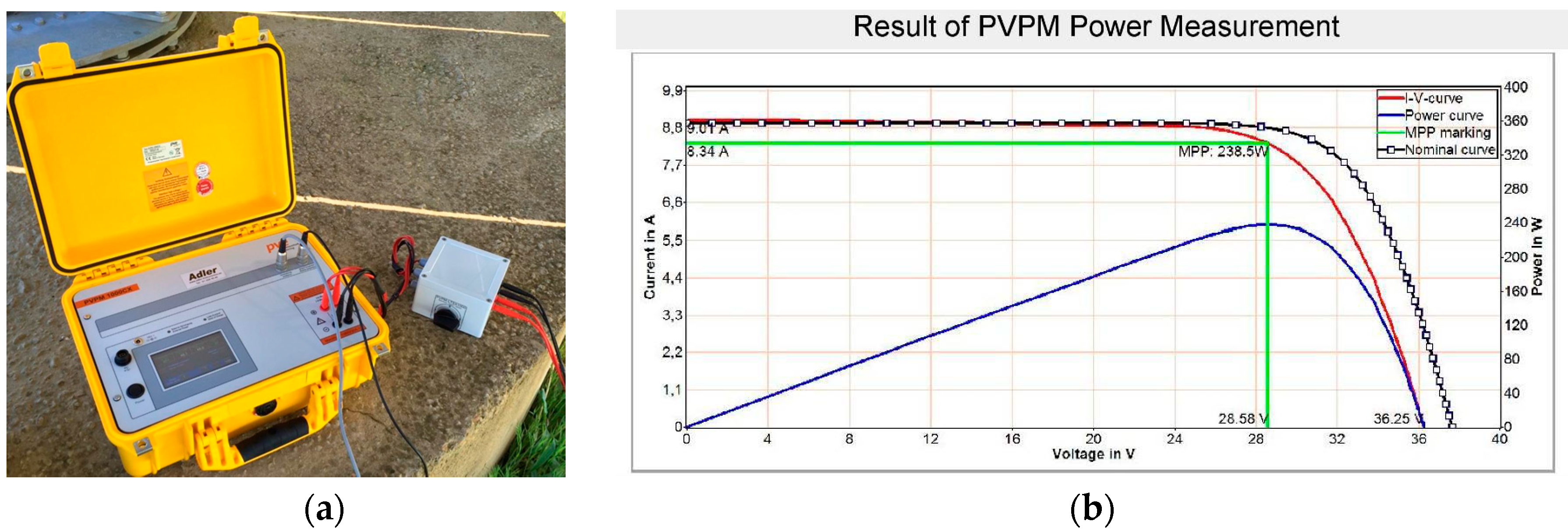
The measurement of the electrical parameters was done with a PV curve tracer brand PVPM1000CX PVE with a NES Solar Radiation Sensor type SOZ-03 calibrated by a First Class pyranometer according to the WMO proposed methodology. The irradiance sensor includes an optimal temperature probe Pt100 mounted directly at the back side of the silicon cell of the SOZ-03 with an accuracy according to DIN EN 60751 Class A (±(0.15 °C + 0.002 T)). Moreover, an external temperature sensor Pt100 measures the PV module temperature for the STC correction. This device fulfils the international standard IEC 60904-1 (monocrystalline silicon) [33] and has an accuracy of the a/d converter of 0.25%, a peak power measurement uncertainty of ±5% and a reproducibility of ±2%. The time taken to perform a single measurement with the device is comprised between 20 ms up to 2 s, avoiding the influence of capacitive properties of the module under test and minimizing measurement variations due to unstable weather conditions. Moreover, the PVPM measurement range is 0–1000 V and 0–20 A, allowing string measurements and checks. Thus, applying the algorithm described in [34,35], the STC I-V curve is obtained. Furthermore, all measurements were taken with global irradiance on the generator plane greater than 800 W/m² and deviations lower than 1%. Both the device and an obtained measurement (I-V curve) can be seen in Figure 7.

With the described device, short circuit current (I_sc), open circuit voltage (V_oc), maximum power point current (I_mpp) and maximum power point voltage (V_mpp), can be obtained with a measuring error <1%.

The internal series resistance (R_s) is calculated with a single measured I-V curve and a simulated one, considering the fill factor (FF) is the same for both characteristics [36] and then applying the IEC 60891 procedure [37,38]. Using a simulated I-V curve prevents the variation of the R_s calculation due to the temperature, which has been stated in [39]. Nevertheless, even considering the influence of a slight temperature variation and the noise present in the I-V curve, the overall uncertainty for the determination of the series resistance is deduced to be ±10% and a repeatability of typically 5% [39].

On the other hand, the parallel resistance (R_p) is calculated as the inverse of the slope of the characteristic I-V curve in short circuit conditions. Thus, a linearization in the range between I_sc and a (I_sc-I_mpp) was carried out, where a was optimized by an iterative numerical algorithm minimizing the variation of the R_p result. The evaluation of the accuracy of this method is not as simple as for R_s because the calculation procedure uses a numerical routine. Nevertheless, the obtained results are within the tolerance of the values obtained for the R_s.

For high accuracy determination of the fill factor, Green provides approximate expressions for arbitrary shunt (parallel) and series resistances [40].

Table 2. Maximum measurement uncertainties for the electrical parameters.

Measured Parameter	Max. Uncertainty (%)
STC Peak Power (W)	±5%
STC Impp (A)	±1%
STC Vmpp (V)	±1%
STC Isc (A)	±1%
STC Voc (V)	±1%
Rs (Ohm)	±10%
Rp (Ohm)	±10%
FF (%)	±2%

shows the maximum measurement uncertainties for all measured electrical parameters expressed as percentage of the measured nominal value.

4. Results and Discussion

The developed GIS tool was applied to two case studies in Spain. The first one was a fixed 108 kWp PV plant connected to the grid, operating since mid-2008. The second one was a self-consumption fixed domestic 9 kWp PV plant installed in the rooftop of a single family dwelling. This installation has been in operation since February 2017.

4.1. Implementation on a 108 kWp PV Power Plant

This plant is operated by the Spanish company Sobarriba Leon 0, and it is characterized by 100 kW nominal power on the inverters and 108 kWp of installed PV modules. It constitutes part of a greater PV plant of 1 MW. Thus, it shares a transformation center formed by two 630 kVA transformers.

In this case, the PV modules are installed on fixed structures, pointing in the southerly direction and tilted 28 degrees with the horizontal surface. The structures are made of steel and foundations are of concrete.

The PV field in this case consists of 432 GFM 220-250 monocrystalline silicon modules 250 Wp manufactured by the company Wuxi Guofei Green Energy Source Co., Ltd., Wuxi, China, Their nominal electrical characteristics according to the manufacturer can be seen in

Table 3. Wuxi Guofei Green Energy GFM 220–250 PV module characteristics.

STC Peak Power (W)	STC Impp (A)	STC Vmpp (V)	STC Isc (A)	STC Voc (V)	FF (%)
250 ± 5%	7.96	31.4	8.38	37.2	0.802

. They are organized in 24 strings (see Figure 2) with 18 modules on each, grouped in parallel through string electrical protection boxes. There are six string electrical protection boxes in total. All modules are fitted with adequate fuse protections.

Therefore, 24 strings of 18 photovoltaic modules arrive to the inverter. The selected inverter is an Ingecon Sun Power model, manufactured by Ingeteam, and 100 kW nominal power. The inverter includes surge protection, a galvanic isolation transformer, DC fuses, anti-island with automatic disconnection protections, a thermal breaker, a reverse polarity protection, a protection against short-circuits, and a protection against insulation faults.

The developed GIS tool allows the analysis of the spatial PV degradation and defect location in an easier way than a traditional statistical analysis. Figure 8, Figure 9, Figure 10, Figure 11, Figure 12, Figure 13, Figure 14, Figure 15, Figure 16 and Figure 17 show the results of the GIS tool for the analyzed electrical parameters. On the other hand, Figure 18 shows the histograms of the measured parameters transformed to STC conditions.

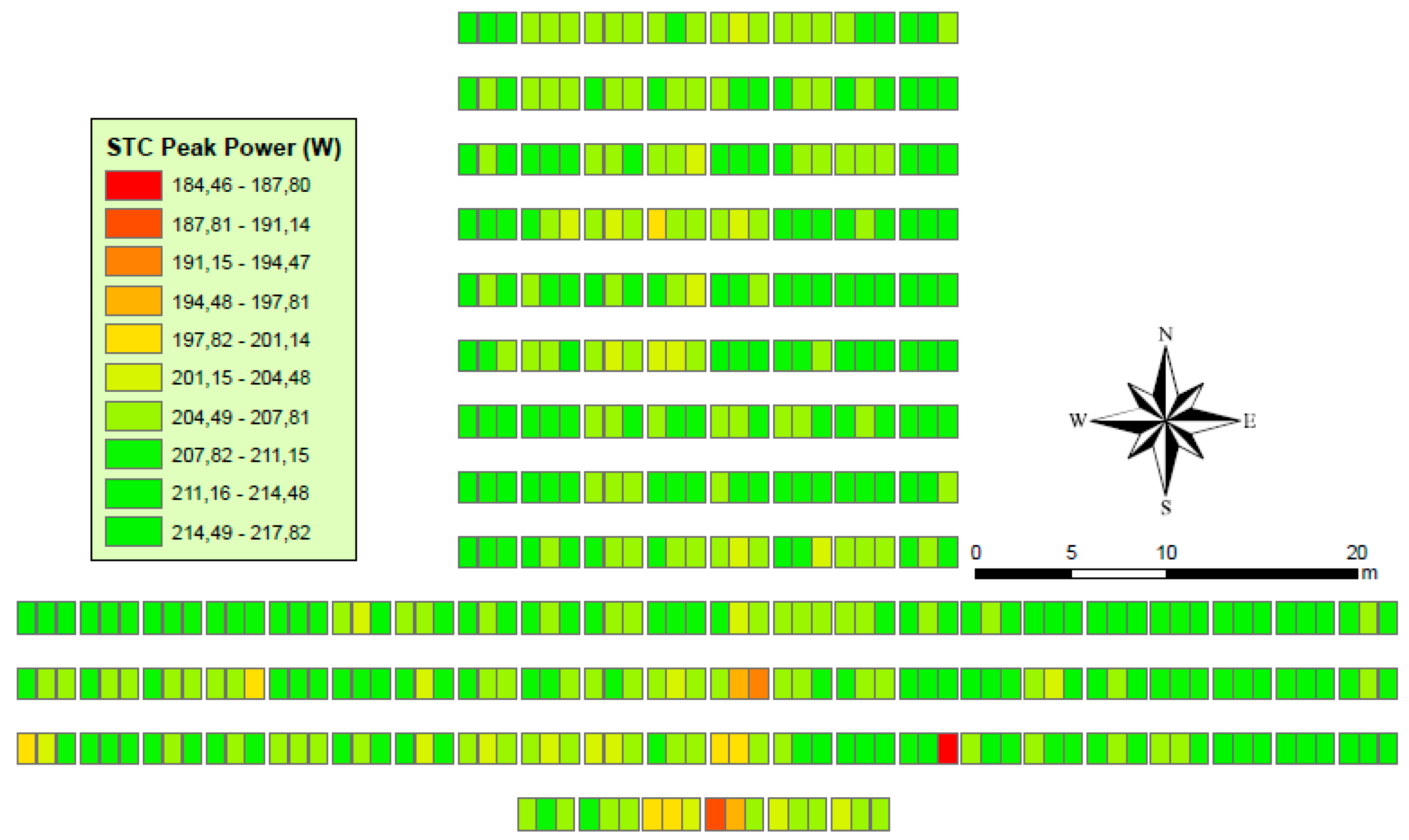
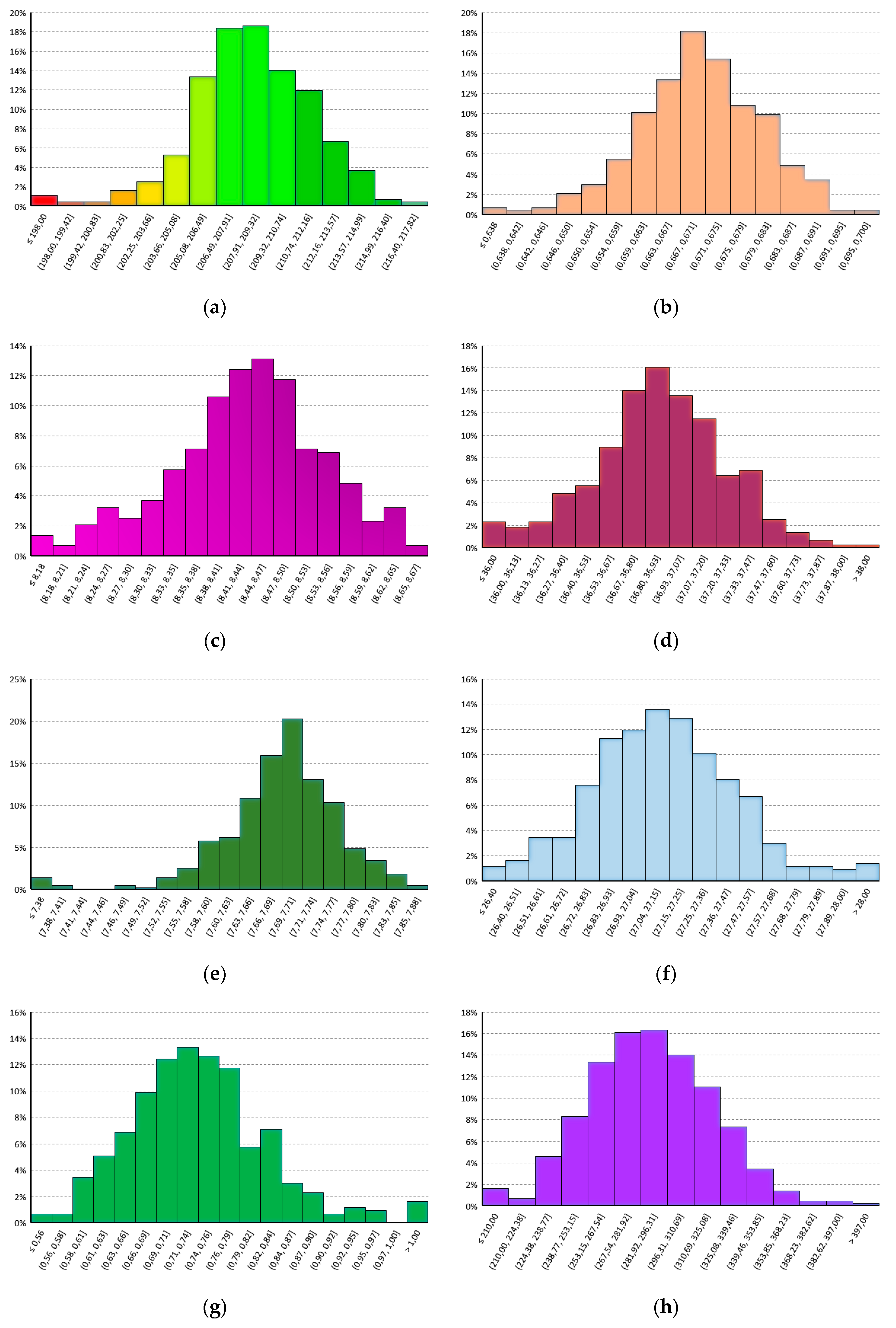
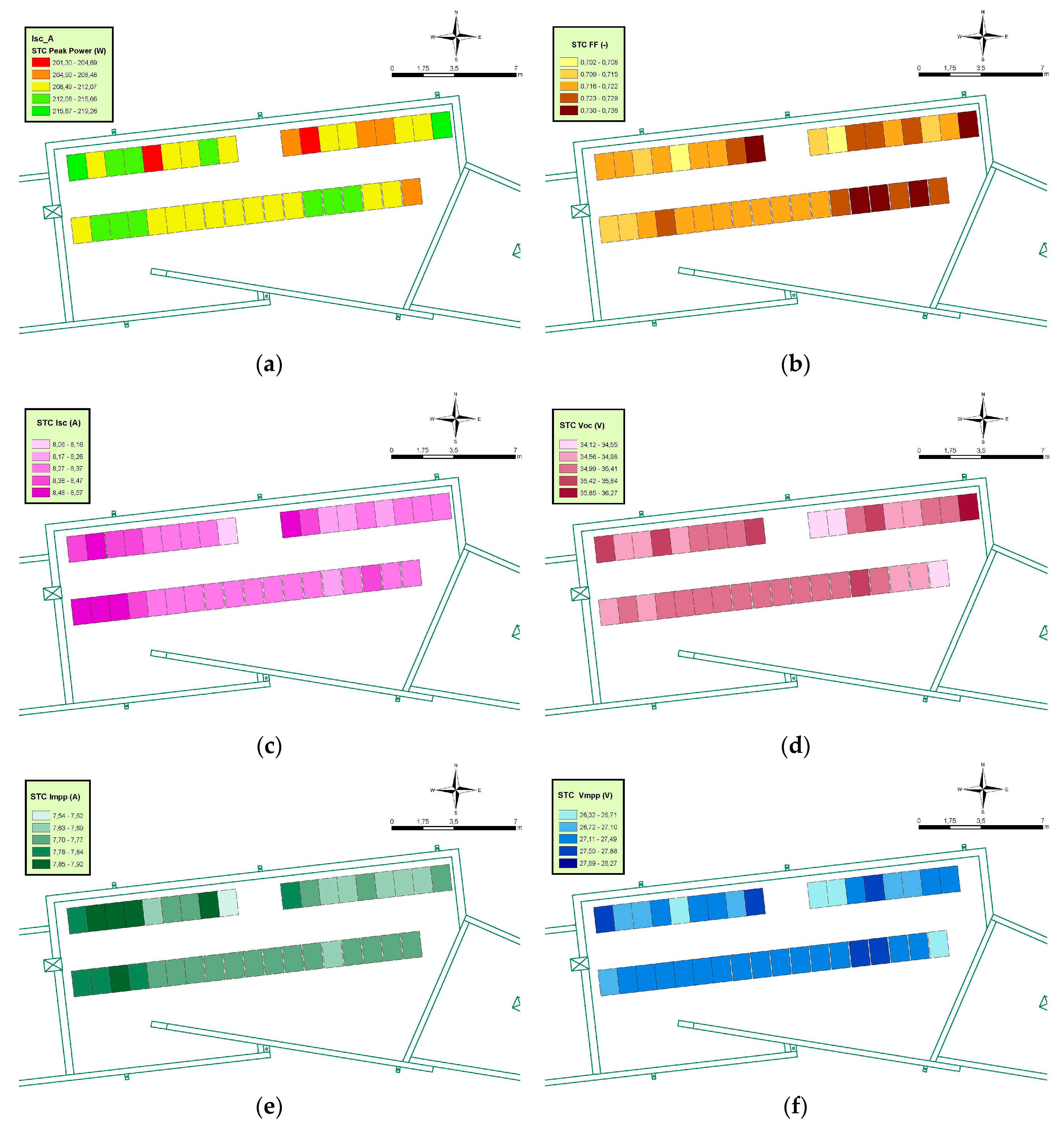
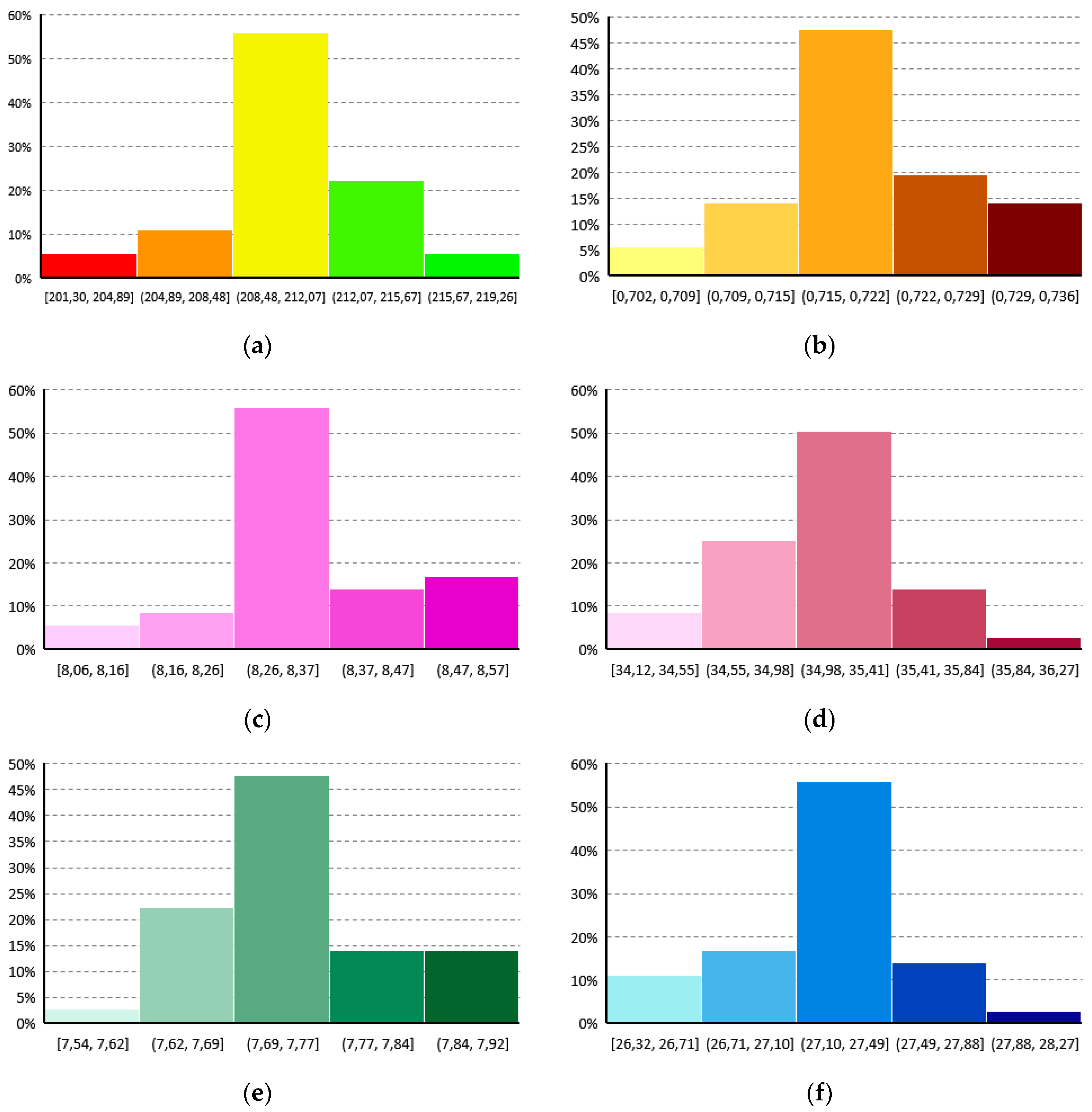
Figure 8 shows lower peak power values for STC conditions in the center of the lower part of the installation, whereas the extremes show significantly higher values. This effect may be caused by the temperature distribution through the PV modules and the refrigeration by air convection conditions. The lowest STC peak power was 184.46 W, where the highest value was 217.82 W (18.09% difference). Figure 18a shows the distribution of the peak power values, where it can be noticed that more than 70% of the modules are in the 205–211 Wp range.

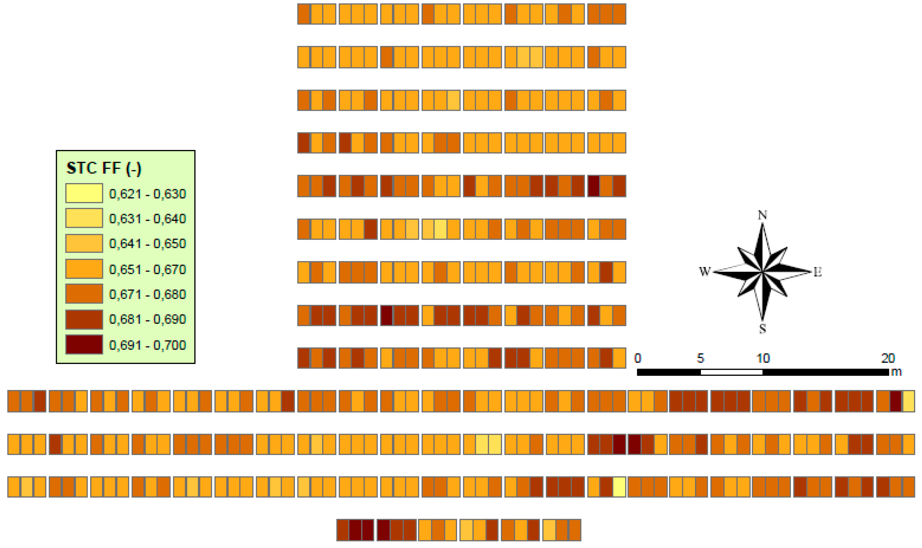
In a similar way, Figure 9 shows the fill factor of the PV modules transformed to the reference STC. Figure 18b shows the histogram for these values. It can be noticed that the PV modules are affected by a significant rate of degradation where 80% of the modules are in the range 0.66–0.68, when the nominal fill factor (FF) given by the manufacturer achieves 0.8018 (see Table 3). Less than 1% of the PV modules present a FF > 0.695. Moreover, it can be observed that those modules with lower values for peak power in Figure 8 show also lower values of FF in Figure 9. However, higher variations of the FF can be noticed in this late figure rather than on the peak power analysis. The fill factor distribution shows not to be homogeneous in the installation and, thus, modules with high values of FF are linked to modules with very low values for FF. Some cases show differences up to 10.53%. This may affect significantly the overall performance of the string series.

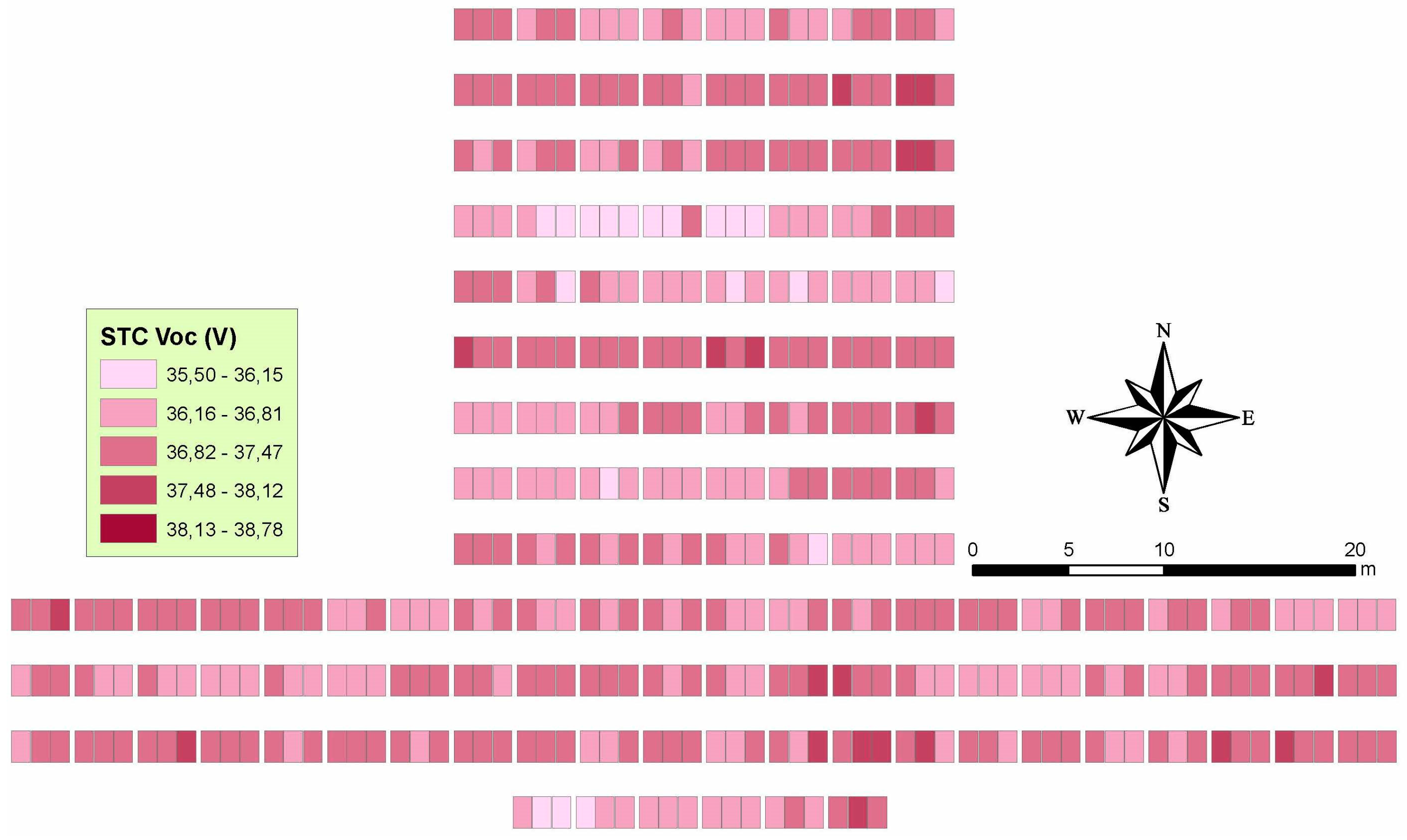
Figure 10 and Figure 11 show the STC short circuit current and STC open circuit voltage distributions respectively. Moreover, Figure 18c,d shows their histograms. From these figures it can be observed that there exist very slight variations on the short circuit distribution (0.6 A max), but significant variations (up to 3.28 V) in the open circuit voltages. Both distributions in the spatial field are absolutely not homogeneous.

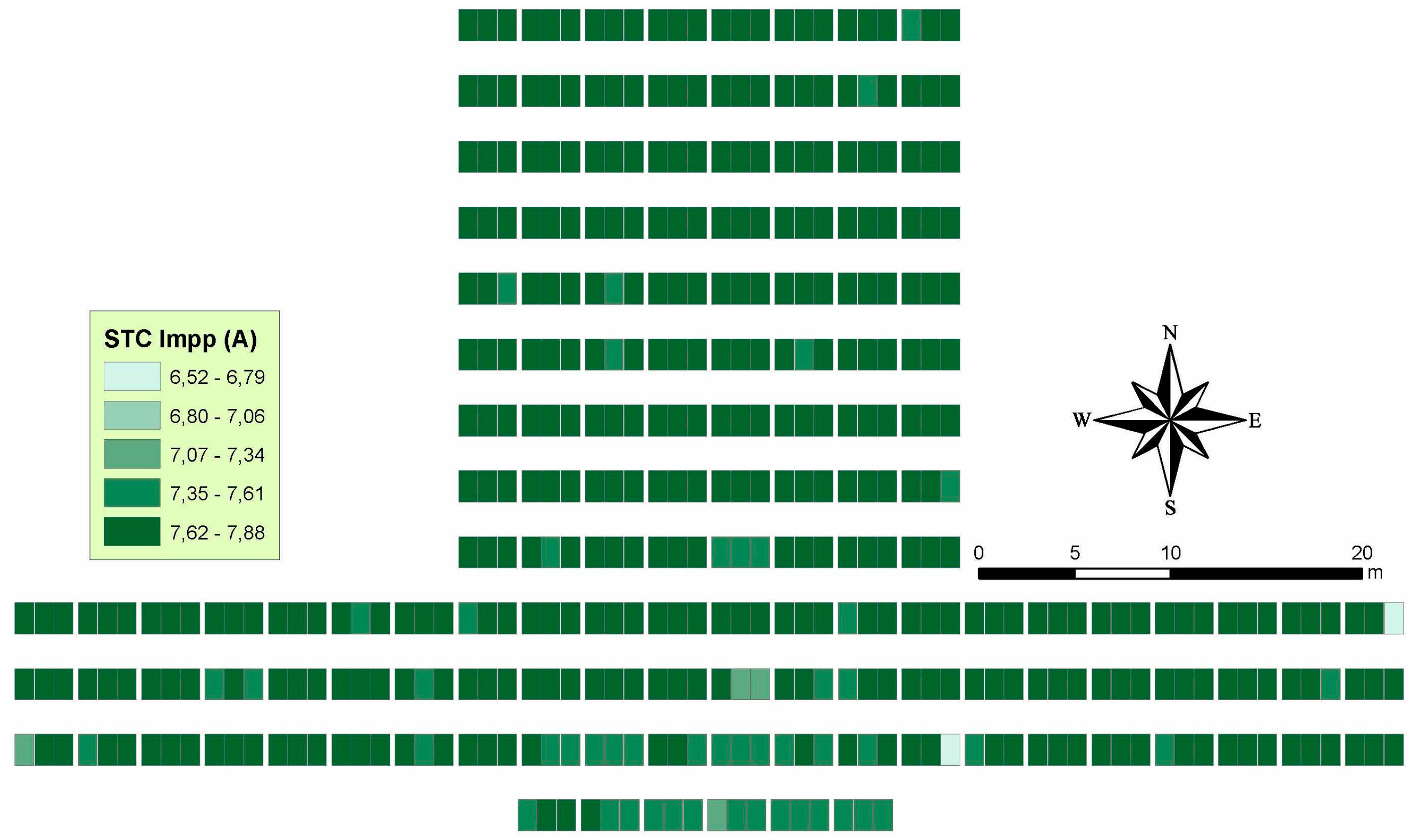
Figure 12 shows a uniform distribution of the STC maximum power current distribution apart from few PV modules which show current values in the range 6.52–6.79 A, while the average, according to Figure 18e is 7.67 A, which is 3.56% lower than the nominal I_mpp.

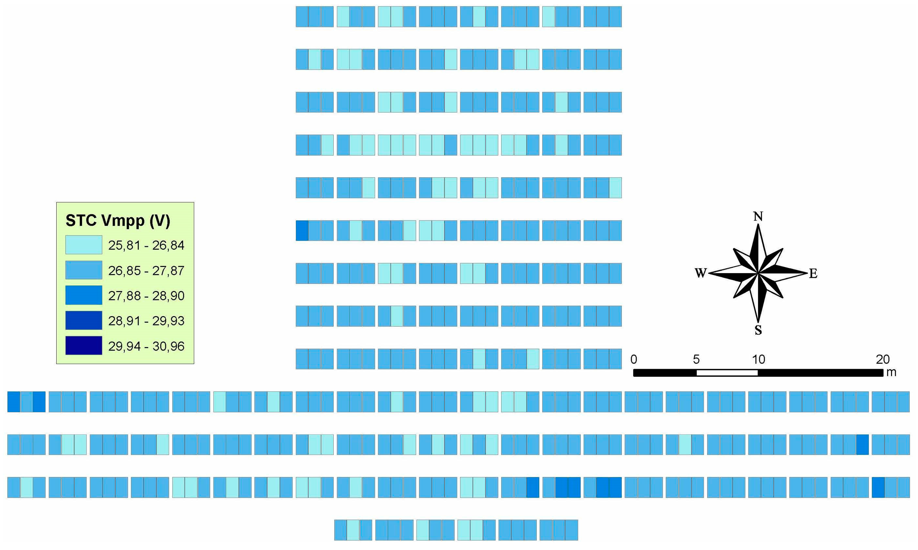
Figure 13 shows the STC maximum power voltage distribution. In this case, the distribution seems to be less homogeneous than the one seen for the maximum power current. Lowest maximum power voltage modules, in the range 25.81–26.84 are located in the northern and center parts of the PV plant, while certain modules located in the second row from the south show a higher voltage value. The histogram for this parameter, which can be seen in Figure 18f shows a distribution close to the normal, with less than 4% of the voltage values higher than 27.68 V and less than 3% of the values lower than 26.40 V.

In Figure 12 the STC maximum power current can be easily distinguished between the groups of PV modules with high values. Distribution on the PV field of this electrical value is not uniform and low values can be correlated with low values of the STC maximum power voltage in Figure 13. Undoubtedly, those PV panels must be inspected with special caution. It can be noticed that higher differences in this value between close located PV modules can be found than when analyzing the maximum power voltage distribution.

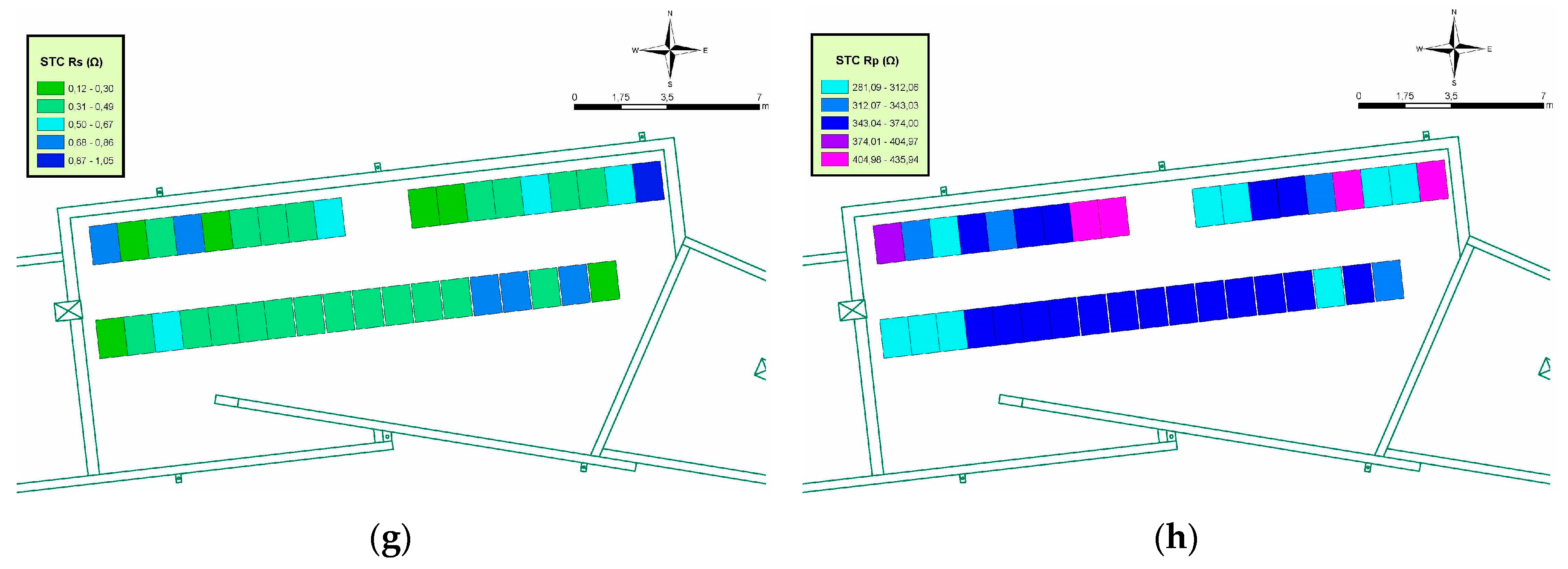
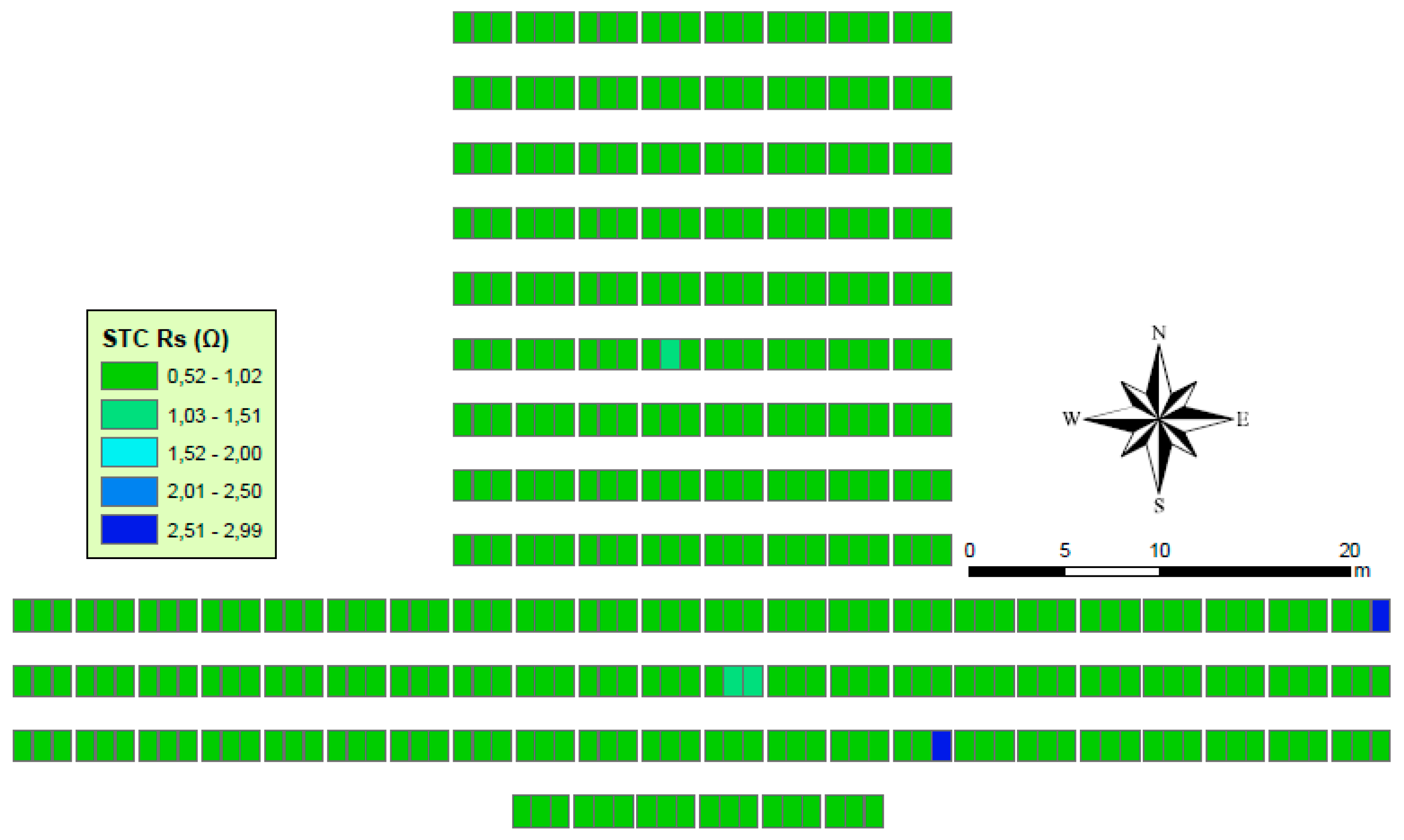
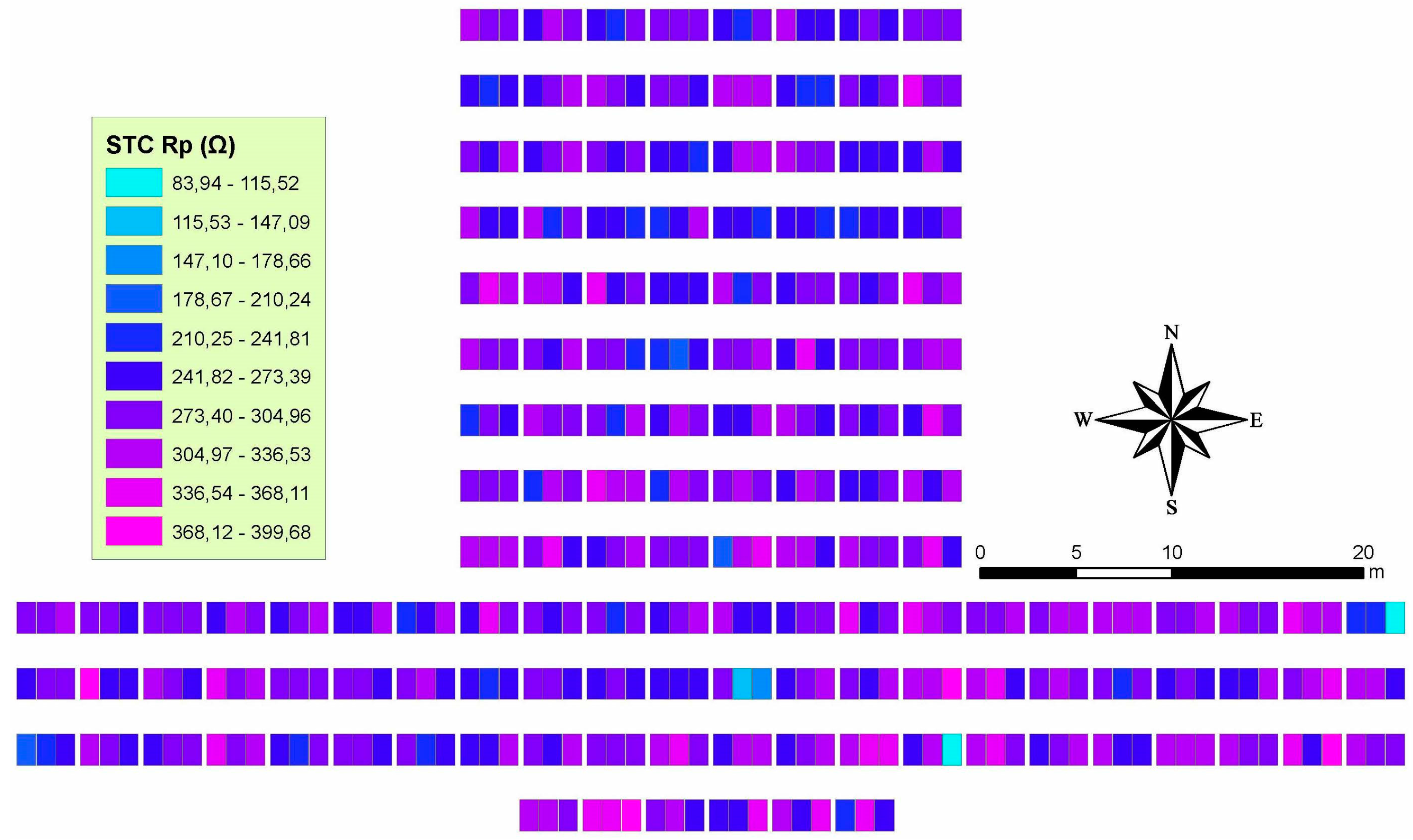
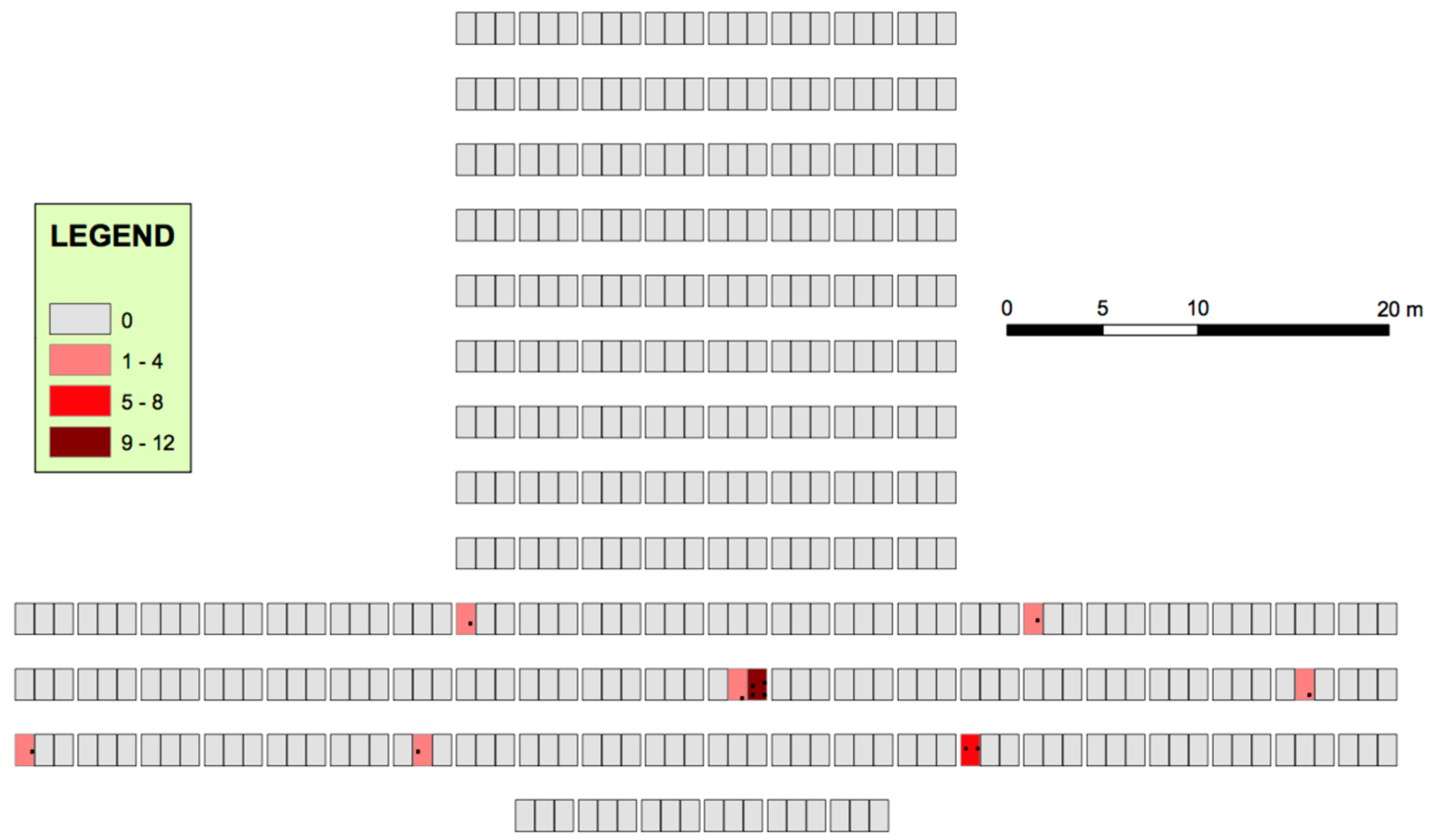
Figure 14 and Figure 15 show the distributions of the series resistance and parallel resistance of the PV modules respectively. Although both distributions are not the same, extreme values are located on the same PV modules. As can be verified in Figure 15, these modules which have high values of series resistance and abnormally low values of parallel resistance, also present a significant high number of hot spots and burn marks (between 1 and 8). Moreover, according to Figure 8, these modules have very low power output. Thus, the whole string series production is affected. These PV panels must be replaced immediately. Fortunately, the rest of the series seem not to have been affected seriously. Figure 18g,h shows the histograms for both electrical parameters. The average for the series resistance is 0.7515 Ohm, while for the parallel resistance it is 286.1831 Ohm. Both values are significantly different (higher in the case of the series resistance and lower for the parallel resistance) from the nominal ones, leading to a considerable degradation rate.

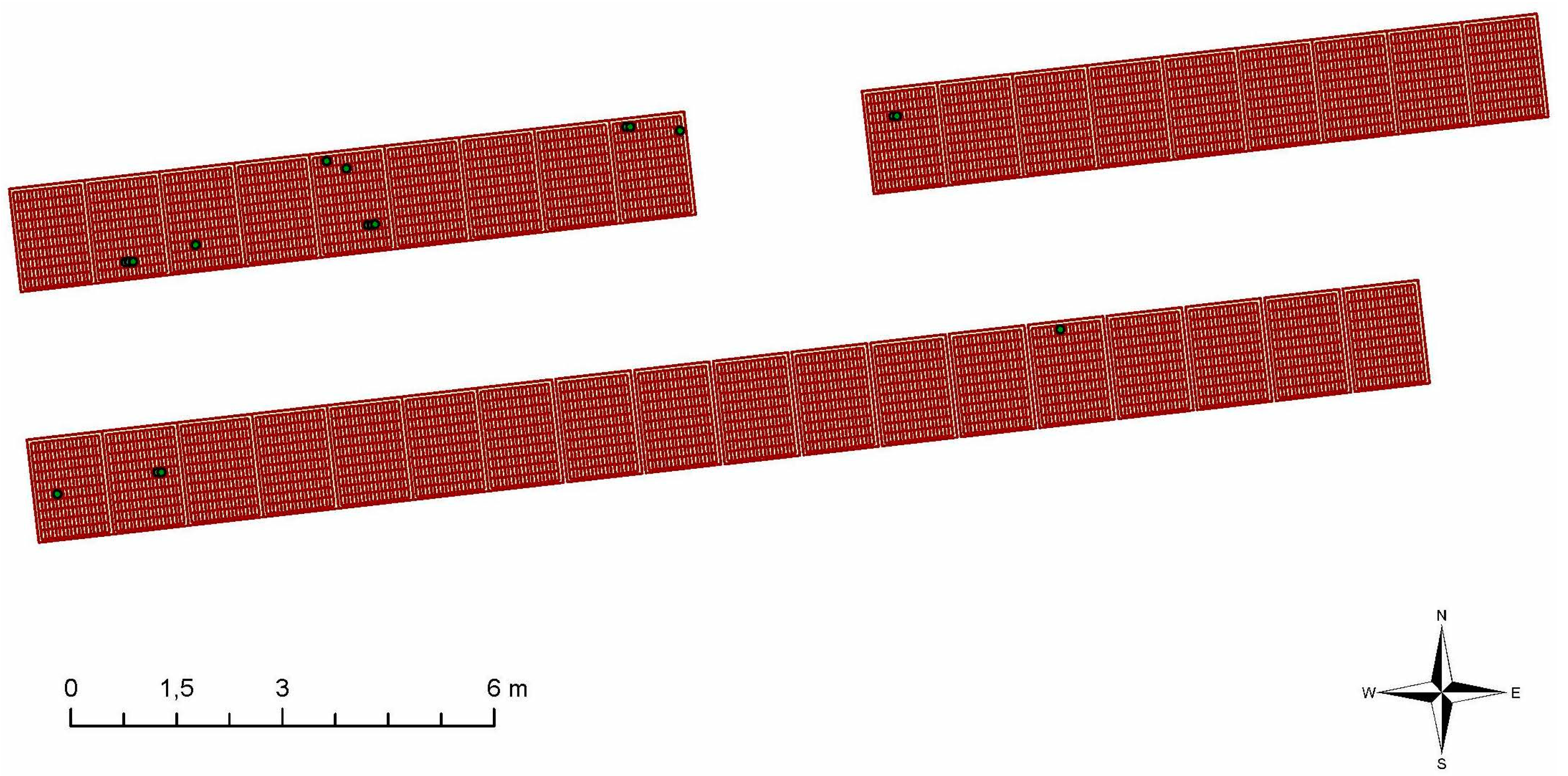
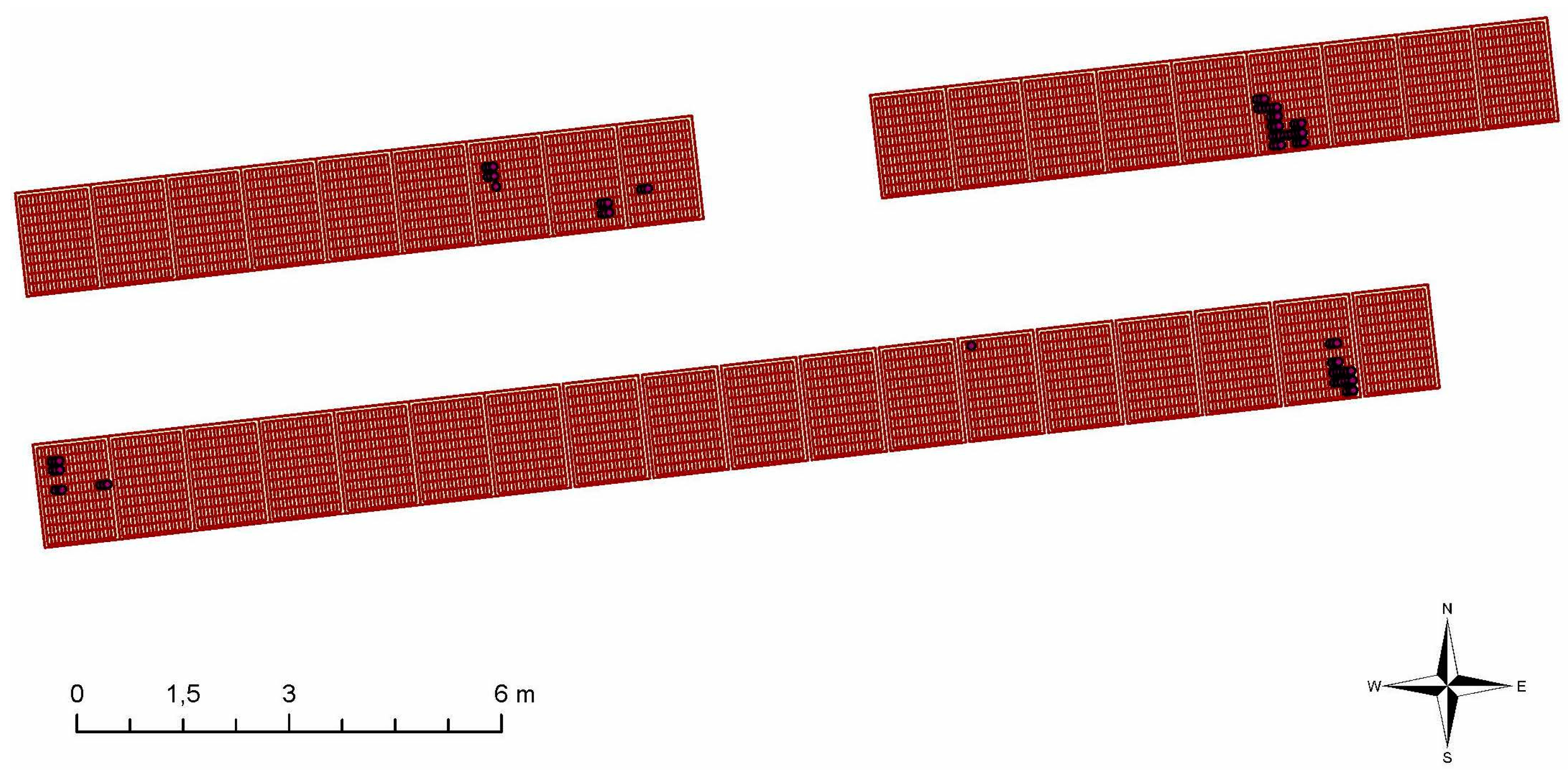
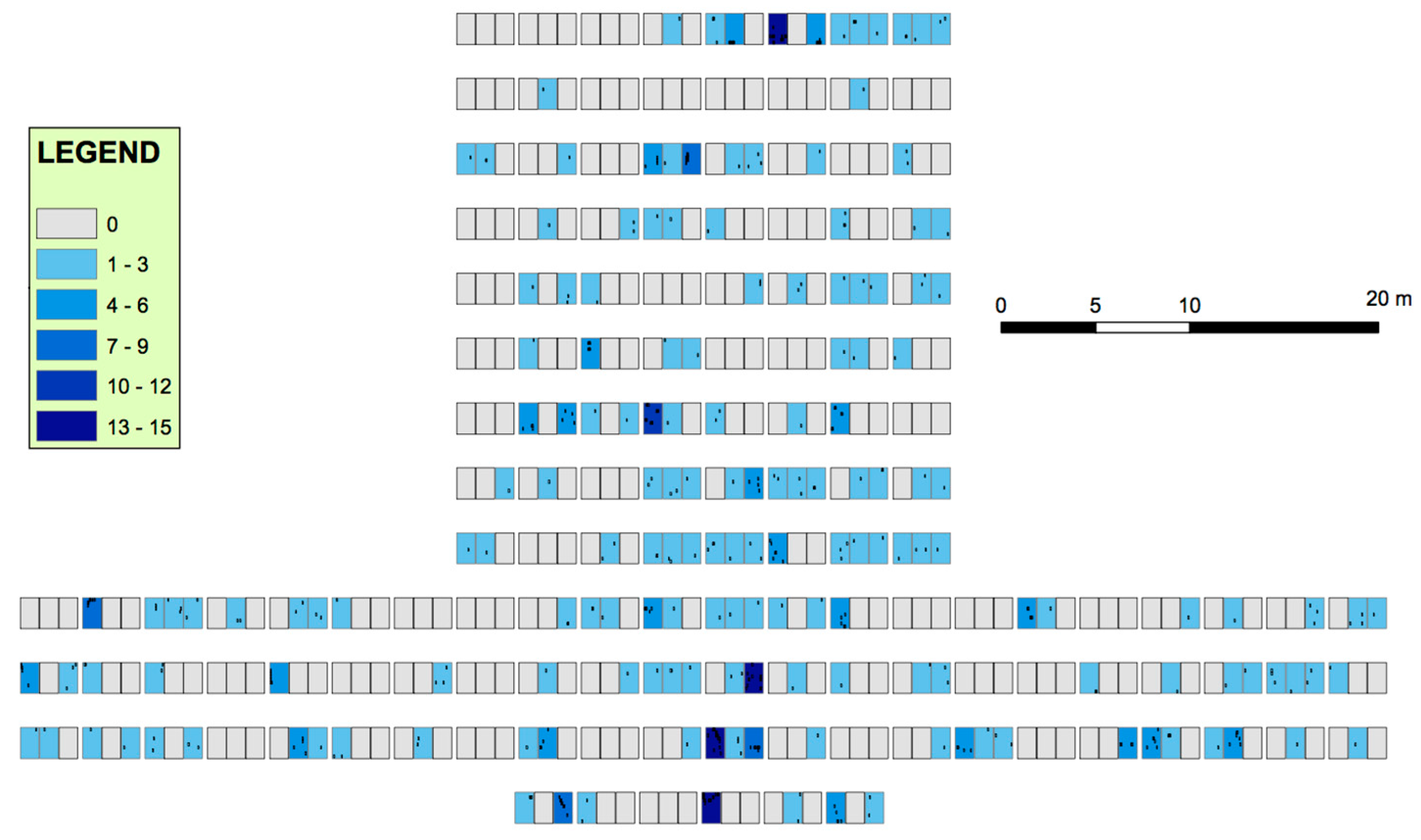
Figure 16 and Figure 17 include the most relevant PV defects on the installation: snail tracks and hot spots and burn marks. The snail tracks distribution in the power field seems not to be homogeneous but we cannot also infer a clear high density zone. PV modules affected by this PV fault seem to have from 1 to 3 defects. However, 15 defects of this type can be found on single modules. No significant correlations with electrical measurements are detected in this case.

Figure 17 shows the hot spots and burn marks found on the PV modules. Fortunately, very few of these defects were found in the installation. In this case, its distribution is clearly concentrated in the lowest part. Moreover, it is remarkable that the module with the highest number of hot spots and burn marks is also the one with the highest number of snail tracks. Its STC peak power output is also lower than the average.

By analyzing Figure 8 and Figure 16, it can be observed that snail tracks may significantly affect the power generation. Some modules with a high number of snail tracks show lower peak power values on STC. However, the thermographies did not detect significant variations on the PV module performance.

The rest of the defects are almost negligible in the power plant. Thus, no GIS tool images have been included but the Summary

Table 4. Found PV defects and associated average electrical parameters values.

	Snail Tracks	Cell Cracks	Hot Spots and Burn Marks	Blue Cells	Bubbles	Busbars Discolorations	Cells Discolorations	EVA Discolorations
# Defects	418	9	36	540	3	4863	4140	40
# Modules	173	4	8	3	2	28	23	4
STC Peak Power (W)	208	207	204	206	207	207	209	207
STC Impp (A)	7.67	7.65	7.48	7.55	7.63	7.63	7.69	7.66
STC Vmpp (V)	27.1	27.1	27.2	27.2	27.2	27.1	27.2	27.1
STC Isc (A)	8.43	8.40	8.38	8.18	8.32	8.38	8.43	8.45
STC Voc (V)	36.9	36.7	36.8	37.0	36.5	36.9	36.9	37.1
Rs (Ohm)	0.77	0.73	0.90	0.67	0.65	0.75	0.72	0.81
Rp (Ohm)	283	291	238	355	312	290	294	272
FF (%)	0.67	0.67	0.66	0.68	0.68	0.67	0.67	0.66

# Indicates number of.

and

Table 5. Found PV defect correlations. Upper mid (above the main diagonal) refers to the number of found defects while the lower mid (below the main diagonal) is refers to the number of modules.

	Snail Tracks	Cell Cracks	Hot Spots and Burn Marks	Blue Cells	Bubbles	Busbars Discolorations	Cells Discolorations	EVA Discolorations
Snail tracks	418/173	0	7	0	0	42	18	0
Cell cracks	0	9/4	5	0	0	0	6	0
Hot spots and burn marks	2	2	36/8	0	0	12	6	0
Blue cells	0	0	0	540/3	0	0	0	0
Bubbles	0	0	0	0	3/2	0	1	0
Busbars discolorations	10	0	1	0	0	4863/28	180	0
Cells discolorations	8	2	2	0	1	1	4140/23	0
EVA discolorations	0	0	0	0	0	0	0	40/4

do include them.

Table 4 shows the average values of the measured electrical parameters for each defect. On the other hand, Table 5 shows the correlations between found defects. This latter table is organized in such a way that it provides two values of interest. The upper mid above the main diagonal includes the counts of the cell parts affected simultaneously by two defects, while the lower mid below the main diagonal includes the counts of modules with both defects. Thus, it can be observed if a module is affected by several defects (lower mid) whether they appear in the same PV cell part or whether they are distributed throughout the module.

Table 4 shows that the lowest average STC peak power is associated with the modules affected by busbar discolorations, provoked by both significant diminutions of the maximum power current but not on the maximum power voltage. The series resistance and the parallel resistance also seems to be significantly affected in this case, but very few differences can be observed for the FF in comparison with the rest of the PV modules defects.

PV fault correlations are shown in Table 5. The results show very few correlations between defects. However, it can be observed that a high number of snail tracks are produced on the same third cell compared to busbar discolorations and cell discolorations. These results also show a strong relationship between hot spots and burn marks with busbar and cell discolorations. PV modules affected by hot spots and burn marks also show a certain correlation with snail tracks and cell cracks.

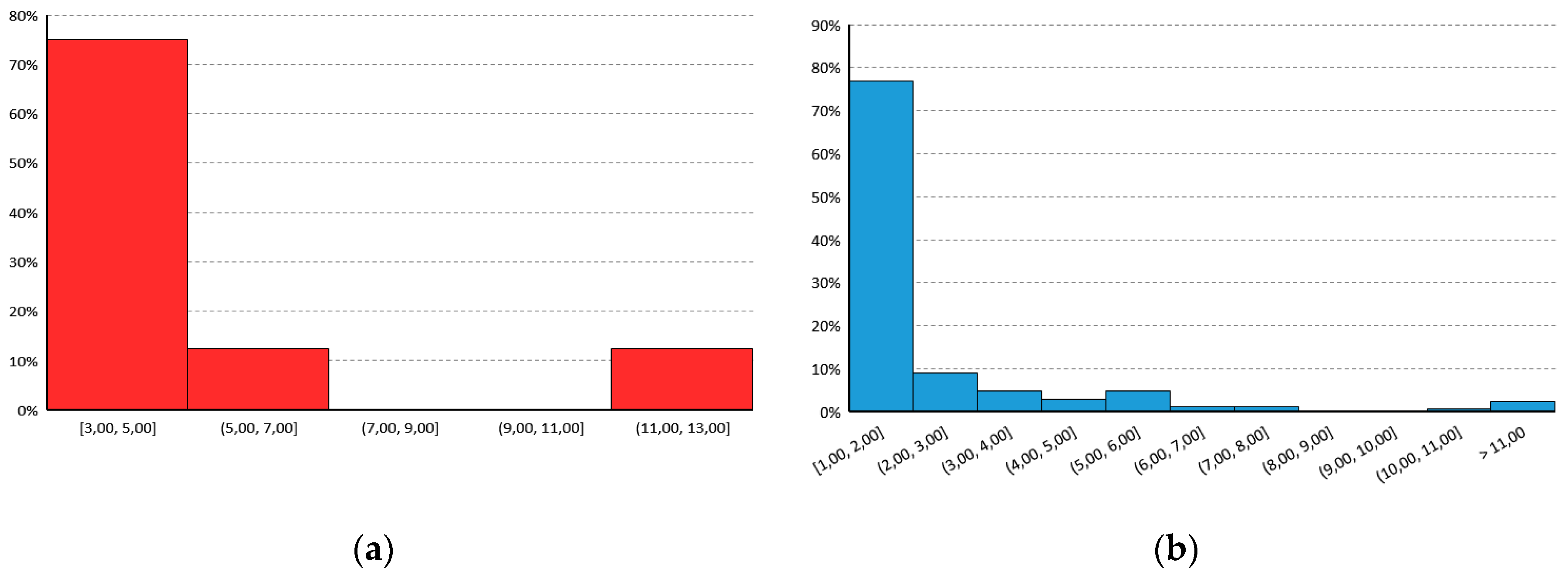
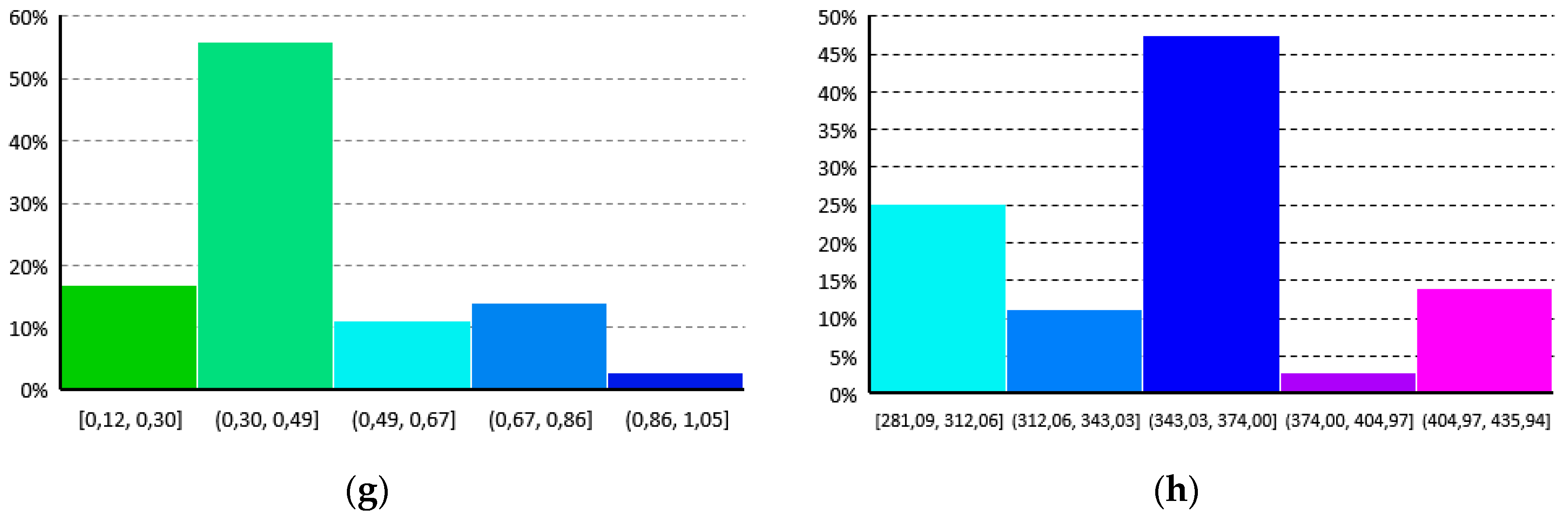
Figure 19 shows both histograms for the hot spots and burn marks (a) and for the snail tracks (b) found in the power plant. Both histograms are expressed in relative terms for the modules affected by the considered fault. PV modules affected by hot spots and burn marks, near 80%, show between three and five faults simultaneously. The other 20% of damaged modules have a greater number of faults with a maximum record of 13 hot spots on a single module. On the other hand, Figure 18b shows that 80% of the PV modules affected by the snail track fault have no more than two faults. Less than 1% of the PV modules damaged this way show more than 11 faults.

Finally,

Table 6. Degradation analysis on the 108 kWp PV plant. Variation of the measured values with respect to the nominal ones. Results expressed in %.

	Unharmed	Snail Tracks	Cell Cracks	Hot Spots and Burn Marks	Blue Cells	Bubbles	Busbars Discolorations	Cells Discolorations	EVA Discolorations	Weighted Average
Peak Power	−16.5	−16.8	−17.1	−18.6	−17.7	−17.2	−17.3	−16.4	−17.1	−16.7
Impp	−3.31	−3.64	−3.89	−6.03	−5.15	−4.15	−4.15	−3.39	−3.77	−3.56
Vmpp	−13.6	−13.6	−13.8	−13.4	−13.3	−13.5	−13.8	−13.5	−13.8	−13.6
Isc	0.77	0.60	0.24	0.00	−2.39	−0.72	0.00	0.60	0.84	0.61
Voc	−0.79	−0.94	−1.26	−1.16	−0.65	−1.83	−0.91	−0.94	−0.38	−0.87
Rs	169	181	167	229	145	137	174	163	196	174
Rp	−42.8	−43.8	−42.1	−52.8	−29.5	−38.0	−42.5	−41.7	−46.0	−43.2
FF	−16.4	−16.4	−16.4	−17.7	−15.2	−15.2	−16.4	−16.4	−17.7	−16.5

summarizes the observed degradation on the 108 kWp PV plant by the variation of the measured electrical parameters with respect to the nominal ones. The weighted average degradation of the peak power is close to 17%, meaning an average linear degradation rate of 1.86%/year. Unharmed PV modules show a lower degradation rate of 16.49%, while the higher degradation is shown on those PV modules affected by hot spots and burn marks (18.56%). The variations found on short circuit current and open circuit voltage are almost negligible, but significant worsening of the series and parallel resistance values are observed.

4.2. Implementation on a 9 kWp PV Power Plant

The second case study is a self-consumption PV power plant operated by the Spanish company Himalaya Sol. It is a fixed 9 kWp plant installed in the rooftop of a single family dwelling. It started operation in February 2017 and consists of 36 GFM 220–250 monocrystalline silicon modules manufactured by the company Wuxi Guofei Green Energy Source Co., Ltd. (see Table 3). The PV modules are installed in a fixed structure with a slope of 32 degrees and oriented 6 degrees East azimuth angle. The modules have a unit peak power of 250 W and its power output is optimized by a P300 optimizer from Solar Edge, as the installation is affected by a high number of shadows (due to the architectural configuration).

The PV modules are organized in three series strings which consist of two strings of 13 modules and one string of 10 modules. The power output from each string is transformed from DC to AC by a 3 kW nominal power inverter manufactured by Solar Edge. Each inverter includes the necessary protections.

As the energy injection to the power grid is not allowed in this installation (it has been regularized as Type 1 self-consumption facility according to [41]) a relay regulates and/or disconnects the power plant in case the consumption becomes lower than the power output.

Due to the novelty of the installation, only the preliminary analysis was carried out in this case. Thus, only the initial modules test and the geodatabase generation were done.

An analysis similar to the previous one can be conducted in this case. However, results for the implementation in the 9 kWp PV power plant have not yet much relevance. As the installation started working recently almost no degradation was observed. However, Figure 20 and Figure 21 show several snail tracks and cell discolorations that may lead to more detailed maintenance needs on these modules. Distributions of both defects are clearly not homogeneous and they seem to be concentrated on the string series extremes.

Figure 22 shows the electrical measure distributions for the second case study. The distributions in all cases are more homogeneous than in the previous case study due to the lower rate of degradation. In this case, major variations are found for maximum power current (Figure 22e) short circuit current (Figure 22c) and parallel resistance (Figure 22h). A correlation between low values of short circuit values and cell discolorations can be found in this case.

Table 7. Found PV defects and associated average electrical parameter values.

	Snail Tracks	Blue Cells	Busbar Discolorations	Cell Discolorations
# Defects	18	36	1	83
# Modules	8	3	1	7
STC Peak Power (W)	210	212	210	210
STC Impp (A)	7.77	7.78	7.65	7.71
STC Vmpp (V)	27.0	27.3	27.4	27.2
STC Isc (A)	8.41	8.36	8.35	8.28
STC Voc (V)	34.9	35.2	35.2	35.0
Rs (Ohm)	0.34	0.61	0.48	0.42
Rp (Ohm)	323	357	284	368
FF (%)	72.0%	72.0%	71.3%	72.0%

# Indicates number of.

and

Table 8. Found PV defect correlations. Upper mid (above the main diagonal) refers to the number of found defects while the lower mid (below the main diagonal) refers to the number of modules.

	Snail Tracks	Blue Cells	Busbar Discolorations	Cell Discolorations
Snail tracks	18/8	0	0	0
Blue cells	0	36/3	0	0
Busbar discolorations	0	0	1/1	0
Cell discolorations	2	0	0	83/7

show the results for the 9 kWp PV plant. In this case, only four defects were found: snail tracks, blue cells, busbar discolorations, and cell discolorations. Relative apparition rates are not similar to those observed in the previous case study. This fact results in thinking of a spatially and temporally spread process. It can be also observed that, in this case, the impact of the blue cells defect on the STC peak power is much lower than in the previous case. Moreover, although both installations have similar fill factor values for the PV modules, in the second case, higher maximum power current values were measured than in the first case, but lower maximum power voltages.

Parallel resistances are higher in the second installation than in the first one for all classified defects, but not for the busbars discoloration fault. On the other hand, series resistance values are significantly lower than in the first case, but for the blue cells fault they are found to be similar.

Figure 23 shows the histograms for the measured electrical parameters for the case study. In this case, dispersions of the values are lower than for the 108 kWp power plant and, thus, fewer bins are identified. Figure 23a shows that the average STC peak power is 210.77 Wp and less than 5% of the modules have less than 204.89 Wp. On the other hand, the fill factor for the PV modules installed in this plant have a higher value, closer to the nominal one. Eighty percent of the PV modules have a fill factor in the range between 71% and 73%.

Figure 23c–f shows the histograms for I_sc, V_oc, I_mpp, and V_mpp, respectively. Dispersion of these parameters is too low and no high differences with the nominal values are observed.

Finally, Figure 23g,h shows the histograms for the series and parallel resistances. Fifty-five percent of the modules have a series resistance in the range between 0.30 and 0.49 ohms, while for the parallel resistance, 47% are in the range between 343 and 374 ohms, but a significant 25% of the modules have a parallel resistance lower than 312 ohms.

Table 8 shows the correlations between PV defects in the second case and it is organized in the same way as Table 5. In this case, only two modules presented both snail tracks and cell discolorations. This is in accordance with the result obtained in the first installation where a high number of PV modules affected by cell discolorations also presented snail track defects.

Finally,

Table 9. Degradation analysis on the 9 kWp PV plant. Variation of the measured values with respect to the nominal ones. Results expressed in %.

	Unharmed	Snail Tracks	Blue Cells	Busbar Discolorations	Cell Discolorations	Weighted Average
Peak Power	−15.5	−16.0	−15.1	−16.2	−16.1	−15.7
Impp	−2.69	−2.39	−2.26	−3.89	−3.14	−2.71
Vmpp	−13.1	−14.0	−13.1	−12.7	−13.4	−13.3
Isc	−0.47	0.36	−0.24	−0.36	−1.19	−0.41
Voc	−5.65	−6.16	−5.51	−5.30	−5.99	−5.80
Rs	81.9	24.1	122	75.2	53.3	67.5
Rp	−31.0	−35.9	−29.2	−43.7	−26.9	−31.4
FF	−10.0	−10.2	−10.2	−11.1	−10.2	−10.1

summarizes the observed degradation on the 9 kWp PV plant by the variation of the measured electrical parameters with respect to the nominal ones. The weighted average degradation of the peak power is close to the 15.7%. Unharmed PV modules show a lower degradation rate of 15.50%, while the higher degradation is shown on those PV modules affected by cells discolorations (16.08%). The variations found on short circuit current and open circuit voltage are almost negligible, but significant worsening of the series and parallel resistance values is observed.

5. Conclusions

The designed GIS tool has proven to be useful to analyze the degradation effects on a PV field and the most common PV defect locations and correlations. Although its implementation has provided useful information for both case studies, its application to big plants seems to be more profitable that for small installations, but higher efforts are required.

The results show no straight correlations between PV defects, snail tracks and cell cracks with different types of discolorations. On the other hand, the electrical parameters on the modules seem not to be uniformly distributed in the power plant and no correlations with defects can be found apart from blue cells, which initially were not considered a relevant defect.

For both cases study, the GIS tool has been proved to be helpful to analyze the degradation rates of the PV modules. Moreover, in contrast with other analyzing techniques, the proposed methodology includes information on the spatial distribution of the PV faults, allowing future research to evaluate the impact of mismatching PV modules affected by faults with unharmed ones.

Furthermore, thanks to the available measurements, preliminary preventive maintenance actions can be carried out, such as the replacement of damaged PV modules according to an abnormal presence of faults and/or a poor electrical behavior in the string, redistribution of PV modules according to their performance and development of new specific supervision, cleaning, and maintenance procedures for those modules affected by damaging PV faults, such as blue cells.

The presented GIS tool will become really useful to supervise electrical parameters degradation in the power plant and the defects evolution and distribution in the PV field. Researchers and maintenance service personnel are encouraged to apply this tool to their installations and compare the results. In our case, periodical measurements and inspections will be added to the geodatabase and the real degradation of the PV field will then be fully analyzed. This will lead to more effective preventive maintenance actuations as well as a more economic module replacement strategy and PV aging true valorization.

Moreover, thanks to this GIS tool, a full analysis on the evolution of the behavior of the 108 kWp PV plant through time will be presented in future contributions. Both the faults location and the spatial distribution of the electrical parameters will be commented on and the presence of correlations will be discussed. Based on this information, advanced preventive PV maintenance protocols will be suggested.