
Theoretical Explanations for the Inverted-U Change of Historical Energy Intensity


School of Management, Harbin Institute of Technology, Harbin 150001, China
*
Authors to whom correspondence should be addressed.
Sustainability 2017, 9(6), 967; https://doi.org/10.3390/su9060967
Submission received: 9 April 2017
/
Revised: 26 May 2017
/
Accepted: 1 June 2017
/
Published: 6 June 2017
(This article belongs to the Special Issue Energy Security and Sustainability)
Abstract
:Historical experience shows that the economy-wide energy intensity develops nonmonotonically like an inverted U, which still lacks direct theoretical explanations. Based on a model of structural change driven by technological differences, this paper provides an attempt to explore the underlying mechanisms of energy intensity change and thus to explain the above empirical regularity accompanied by structural transformation, through introducing a nested constant elasticity of substitution production function with heterogeneous elasticities of substitution. According to some reasonable assumptions, this extended model not only describes the typical path of structural change but also depicts the inverted-U development of economy-wide energy intensity. With the availability of Swedish historical data, we take calibration and simulation exercises which confirm the theoretical predictions. Furthermore, we find that: (1) elasticities of substitution may affect the shapes and peak periods of the inverted-U curves, which can explain to a certain extent the heterogeneous transitions of economy-wide energy intensity developments in different economies; and (2) over long periods of time, the economy-wide energy intensity determined by the initial industrial structure and sectoral energy intensity tends to grow upward, while structure change among sectors provides a driving force on reshaping this trend and turning it downward.
1. Introduction
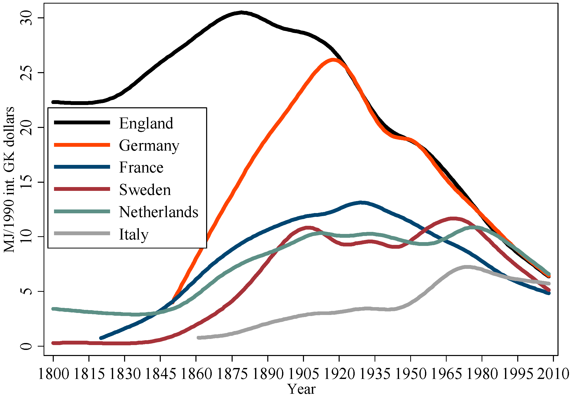
A large number of studies have shown that in the process of industrialization, economy-wide energy intensity universally grows like an inverted U (see, e.g., [1,2,3], or Figure 1). How does this empirical regularity be theoretically explained? To our knowledge, the interpretations of such fact mainly come indirectly from the Environmental Kuznets Curve (EKC) hypothesis (e.g., [4,5,6,7]), with a lack of direct research from inside the economic system. However, this kind of work is of vital importance since the inverted-U change of energy intensity implies that the economic system itself has a dematerialization mechanism that can reduce its dependence on energy endogenously, and mitigate the climate problems eventually. Of course, the environmental and climate problems in the world today may not be able to support this evolutionary mechanism any longer, but when designing appropriate exogenous policies to force energy intensity into downtrend without (overly) damaging economic growth, we should first find out the reasons for the inverted-U development of energy intensity. Alternatively, the exploration of the theoretical explanations for the inverted-U change of historical energy intensity in the industrialized countries may help to formulate efficient energy-saving policies in those developing countries.
Note: (1) Conceptually, energy here denotes modern or commercial energy (i.e., coal, oil, natural gas, and primary electricity), which is in line with references of [1,2,3]; (2) the energy data come from Kander et al. [8] and the GDP data are collected from Maddison [9] at 1990 price level; and (3) all energy intensities are smoothed by Hodrick–Prescott filter with a value of 1600.
The EKC hypothesis generalizes the connection between energy consumption and industrialization, revealing an inverted-U-shaped relationship between environmental quality and economic development. Since energy, especially fossil fuel, has a certain causal link with environmental quality, the theoretical interpretations of EKC hypothesis may also be able to explain the inverted-U development of energy intensity. However, these explanations are based on environmental economics rather than standard growth theories. For example, Kijima et al. [10] pointed out that all EKC models must consider the trade-off problems of pollution, implying that the long-run evolution of energy intensity was driven from outside of the economic system through, e.g., emission abatement expenditures and environmental regulations. Contrarily, the proposed model will theoretically investigate this stylized fact from inside of the economic system under the standard growth framework.
Since the seminal work of Dasgupta and Heal [11], Solow [12] and Stiglitz [13], there has been a strand of literature covering the effect of energy on economic growth, while few of them focused on the long-run growth, not to mention the evolution of energy intensity. For example, Stern and Kander [14] developed a simple extension of the single sector Solow growth model [15] through the inclusion of energy. Further, Kander and Stern [16] extended it by dividing energy into traditional biomass-based energy and modern energy. They derived econometrical models and carried out counterfactual simulations, showing that the expansion of energy played a major role in explaining the economic growth in Sweden. However, they did not explore the dynamics of energy intensity explicitly. Fröling [17] incorporated energy into a unified growth model proposed by Galor and Weil [18] to investigate the role of energy use in world economic development through the transition from stagnation to growth, where energy was produced by aggregating biomass and coal in a constant elasticity of substitution (CES) production function. Moreover, each form of energy took labor as the primary input but used different production technologies; that is, the production of coal was endogenously enhanced by the stock of knowledge while biomass was produced with constant technology. Whereas, the model was only calibrated to predict the world biomass and coal production for the period of 1800–1970, without consideration of energy intensity developments. Eren and Garcia-Macia [19] and Pezzey et al. [20] independently developed two directed technical change (DTC) models, based on the model of Acemoglu [21], to explain British Industrial Revolution. Both models included two energy-using sectors (wood-using sector and coal-using sector) combined in a CES function to analyze the role of energy transition from wood to coal in the Industrial Revolution. However, they did not provide any clear evidence for the change of energy intensity. Tahvonen and Salo [22] investigated energy transition in historical context and showed that the emphasis on energy production might evolve from renewables (i.e., hydropower, wind energy, solar energy, biomass and geothermal energy) to nonrenewables (i.e., fossil fuels) and back to renewables. They then introduced two different growth models, one with constant technology and the other with endogenous technical change, to describe the energy transitions driven by different price paths of the two energy forms at different economic development stages. With numerical examples, they demonstrated that there might exist an inverted-U relation between energy use and economic development (GDP) for the case of constant technology, and an inverted-U relation between nonrenewables and economic development for both cases. However, there are some limitations to this study: (1) it does not analyze energy intensity change explicitly so that more features about the dynamics of energy intensity can not be explored; and (2) energy intensity is in general measured under the concept of total energy rather than nonrenewables only. In this sense, the finding of an inverted-U relation between energy use and GDP seems more attractive, but the assumption of constant technology makes it less interesting and reasonable.
The second relevant strand of literature is concerned with decomposition analyses on the change of energy intensity, which include index decomposition analysis [23,24], structural decomposition analysis [25,26], and production-theoretical decomposition analysis [27,28]. Further, several studies (e.g., [29,30]) also provided the comprehensive decomposition frameworks through integrating some of the above methods to deeply explore the mechanisms of energy intensity change. However, the aforementioned decomposition methods are in nature analytical approaches that aim to disaggregate the overall energy intensity into some specific and meaningful parts to further identify driving forces on the dynamics of energy intensity. In general, these analytical studies neither provide underlying theoretical explanations on the change of energy intensity nor study the specific changing shapes of energy intensity (e.g., U or inverted-U trends).
The third relevant strand of literature aims to explore the change of energy intensity using theoretical approaches. For example, Haas and Kempa [31] first utilized a theoretical model with DTC, marginally modified from the model in Acemoglu et al. [32], to analyze the observed heterogeneous energy intensity developments across countries. Based on this model, the overall energy intensity changes could be theoretically decomposed into structural changes (Sector Effect) and efficiency improvements (Efficiency Effect). In addition, they provided three separate scenarios of energy price growth relative to different historical periods from 1950 on to investigate different trends of energy intensity, including e.g., the inverted-U trend. However, in each scenario of energy price growth, the overall energy intensity grows monotonically. After Cao [33] developed an alternative theoretical model based on the structural change model proposed in Ngai and Pissarides [34] to explore the underlying mechanisms of energy intensity change, featuring in the exploration of nonmonotonic developments (U and inverted-U trends) endogenously. However, the above two theoretical studies mainly focus on the identification of general mechanisms of energy intensity change with two-sector growth models and some numerical examples, but pay no attention to the energy intensity change under the background of industrialization, which is more general and valuable for those developing countries to formulate energy policies.
In this regard, we relate the inverted-U change of overall energy intensity to Kuznets facts (see, e.g., [35,36]) that describe the typical path of structural transformation in the process of industrialization, and analyze how structural transformation leads to the inverted-U evolution of economy-wide energy intensity with a three-sector (agriculture, manufacturing, and services) growth model. That is, we provide an attempt to accommodate these two facts in a unified framework. The basic thought of the connection between the inverted-U change of energy intensity and structural change came from Percebois [37], Reddy and Goldemberg [1] and Panayotou [38]. For example, Panayotou pointed out that the transition from heavy industry to information and service industries could itself explain the inverted-U-shaped link between energy intensity and economic development. This idea has been modeled in the EKC studies (e.g., [7,39,40,41]), however, to our best knowledge, it is first modeled in this paper from the standard-growth-theory perspective. On the other hand, structural change models, aiming at providing possible reasons for long-run structural transformation (e.g., [34,36,42,43,44]), have been used as a benchmark framework to address energy and environmental issues. For example, Stefanski [45] constructed and calibrated a multi-sector, multi-country growth model to evaluate and isolate the impact of changing sectoral composition in developing countries on global oil demand and the oil price in the Organization for Economic Co-operation and Development (OECD) countries. Engström [46] proposed a multi-sector growth model with climate externalities to explore how climate change influenced structural change and both of them influenced the optimal fossil fuel consumption.
Based on the marginally extended version of the models in Ngai and Pissarides [34] and Cao [33], and the availability of Swedish historical data for the period of 1850–2010 [8,47], we investigate: (i) how structural transformation among agriculture, manufacturing and services might take place with a nested CES function; (ii) under what conditions the inverted-U change of overall energy intensity might occur accompanied by structural changes; and (iii) how the turning points of inverted Us might be shaped by heterogeneous elasticities of substitution.
2. Model Economy
Our analysis builds upon the work of economic growth models, especially those providing explanations on the dynamics of structural transformations. There are two different lines of literature concerning structural change models (see, e.g., [48]): the first line is demand-driven, and the second line is supply-driven. This present model is extended directly from the model in Cao [33], and belongs to the supply-driven line that was initiated by Baumol [29] and further developed by Ngai and Pissarides [34], regarding technological differences as the reason for structural change. Specifically, structural change is determined by relative sectoral technological growth rates as well as the elasticity of substitution between sectors. If the elasticity of substitution is bigger than one, the sector of higher technological growth rate will expand faster; alternatively, if the elasticity of substitution is smaller than one, the sector of lower technological growth rate will expand faster.
2.1. Final Good
We consider a simple and closed model economy which competitively produces one unique final good by combining traditional and modern goods with a CES production function following Acemoglu and Guerrieri [43].
where denotes traditional (agricultural) good, and denotes modern good which is produced as follows:
where , denote the output of manufacturing and services, respectively. are distribution parameters, measuring the relative importance of sectoral goods in the aggregate production. are elasticities of substitution between sectoral goods. Accordingly, the final good is eventually produced through a nested CES function, which is quite different from Ngai and Pissarides [34], where the final good is produced by aggregating multiple sectoral goods with a standard CES function. On the one hand, the two-tier nested CES function is more flexible to describe the real economy since values of the two elasticities of substitution can be differently assigned. On the other hand, the incorporation of heterogeneous elasticities of substitution undoubtedly makes the calculation of the model more difficult. To simplify, we instead assume that factor income shares are equal across sectors following Ngai and Pissarides [34], unlike the assumption in Acemoglu and Guerrieri [43], where different factor income shares are assigned to different sectors.
Due to perfect market competition for final and modern goods, producers maximize their profits by choosing the quantities of sectoral goods:
where , , , and denote the prices of final good, modern good, agricultural good, manufacturing good and service, respectively. According to the first-order conditions, we derive:
2.2. Sectoral Goods
There are three different sectoral goods in the model economy, each of which is produced competitively with labor and energy through a Cobb–Douglas production function:
where , are energy and labor inputs of sector , and the superscript denotes the part of total labor employed in the three sectors, i.e., agriculture (), manufacturing () and services (). is sectoral production technology growing at a constant rate with the initial sectoral production technology .
Sectoral goods are produced competitively so that producers choose the quantities of labor and energy to maximize their profits:
where and are wages and energy prices, respectively. Solving the optimization problem, we have:
2.3. Energy
The model economy is assumed to be closed, while some real economies are heavily dependent on energy importing. In view of this, energy here is defined as secondary energy. From this perspective, energy suppliers in this model economy are similar to energy conversion manufacturers, and technological change is reflected by conversion efficiency improvement. Following Gernrnell and Wardley [49] and Fröling [17], the production of energy is given by
where denotes the part of total labor employed in the energy sector. is energy production technology with a constant growth rate and the initial energy production technology .
Energy suppliers are competitive and maximize their profits by choosing the amount of labor:
We solve the maximization problem and have:
3. Structural and Energy Intensity Change
3.1. Structural Change
Referring to Ngai and Pissarides [34], we define structural change as the long-run adjustments of sectoral labor shares.
Integrating Equations (8) and (11), we derive the equilibrium wage-energy price ratio as:
Equation (12) is an analog of Equation (14) in Cao [33], implying that energy–labor ratios are equal across sectors in equilibrium and will grow proportionally to energy technological development, which can be applied to investigate the change of energy intensity next.
Considering the two-tier CES final production function and according to Cao [33], we choose to analyze the production of modern good first and then extend it into the final good production.
Combining Equations (8) and (12), we get:
We then explore the dynamics of Equation (13) by taking the logarithms of both sides and differentiating them with respect to :
where “•” denotes the derivative with respect to . Equations (13) and (14) show that the gaps between sectoral price growth rates are inversely proportional to the gap between sectoral technological growth rates.
Integrating Equations (6), (8) and (12), we get the relative labor ratio between manufacturing and services:
Equation (15) indicates that the relative labor ratio is consistent to the relative output value ratio, implying that variables of labor and output value are equivalent when measuring industrial structure. This connects our theoretical study with the existing analytical studies which generally use output value to measure industrial structure.
Consider the dynamics of relative labor ratio between manufacturing and services from Equation (15):
where , , and . We adjust Equation (15) to obtain a more general expression of sectoral labor share as follows:
With Equations (12) and (17), we can rewrite the modern good production function to be a reduced Cobb–Douglas form:
where , and its production technology and technological growth rates are:
Following the above procedures, we can easily derive the dynamics of the relative labor share between traditional and modern goods:
where
We also find that the final good production function can be reduced to the Cobb–Douglas form:
where , and its production technology and technological growth rates are expressed as:
Equations (16) and (20) indicate that the development of relative labor share between sectors is determined by technological differences amid sectors as well as elasticities of substitution. Furthermore, we can conclude that the necessary and sufficient conditions for structural change in modern (final) sector are and ( and ). When , the sector of higher technological growth rate would expand faster than the other. In contrast, when , the sector of lower technological growth rate would expand faster. Moreover, we note that the technological growth rates of modern and final goods in Equations (19) and (23) vary with structural changes, providing possibilities of nonmonotonic change of energy intensity since the energy production technological growth rate is exogenously given.
According to Kuznets facts, in the long run, the labor share of agriculture goes downward, the labor share of services goes upward, and the labor share of manufacturing goes upward first then downward, like an inverted U. In this sense, we need to make further assumptions to specify the structural transformation of the three main sectors.
Assumption 1.
.
Assumption 2.
, .
Assumptions 1 and 2 come from the Swedish historical data (see in Section 4). In fact, historical energy and GDP data are available in several developed countries (see in Figure 1). However, few of these countries can afford the data of labor (or output) at industry level in a very long period. Sweden is an exception and we choose it as the case study.
Since this study explores structural change and energy intensity change in the long run, technological growth rates and elasticities of substitution may vary in different periods, not only their own values but also the relative magnitudes between sectors. However, for the purpose of modeling and simplifying real economy, we need to make some reasonable assumptions. On the one hand, we suppose that during the development of industrialization, the average technological growth rate of manufacturing keeps the highest, followed by services, and then agriculture. This is different from the assumption in Ngai and Pissarides [34], where the order of manufacturing and agriculture is exchanged relative to this paper. We believe that this divergence is caused by the sample heterogeneity and does not violate the general mechanisms of structural change because the relative magnitudes of sectoral technological growth rates in Ngai and Pissarides were conjectured through USA data from 1929 to 1998, whereas the rankings of technological growth rates among sectors in this paper are conjectured with Swedish data from an even longer period between 1850 and 2010. In General, both sectional and period heterogeneities may lead to differences of the relative technological growth rates. Moreover, when considering the post-war modernization of agriculture in developed countries, it is clear that the sooner the sample period is, the bigger the weight of modern agriculture is, coinciding with the speculations of Ngai and Pissarides. However, the sample period in the present study is much longer, giving more weight on traditional agriculture, so that the technological growth rate of agriculture becomes lower.
Assumption 2 indicates that agricultural and modern goods are gross substitutes (), while manufacturing and service goods are gross complements (). In addition, means that in the final production, the input ratio of goods is more sensitively altered than the price ratio of goods, implying that the adjustments amid agricultural and modern goods are more drastic. On the contrary, indicates that in the modern production, the input ratio of goods is insensitive to the price ratio of goods; that is, the long-run adjustments are relatively slow.
We give the following proposition about structural transformation according to Kuznets facts.
Proposition 1.
Suppose Assumptions 1 and 2 hold in a long enough economic evolutionary process. In the modern (final) production, the labor share of manufacturing (agriculture) declines while that of services (modern sector) increases. In general, during the economic development, the labor share of agriculture tends to decline, the labor share of services tends to increase, and the labor share of manufacturing tends to grow upward first then downward, like an inverted U.
Proof.
See Appendix A.
Comparatively, Ngai and Pissarides [34] provided the necessary and sufficient conditions for structural change implicitly between two sectors with only one elasticity of substitution, while Proposition 1 explicitly describes the typical path of structural change among agriculture, manufacturing and services with two heterogeneous elasticities of substitution.
3.2. Inverted-U Change of Overall Energy Intensity
In this part, we examine the underlying mechanisms of energy intensity change, particularly the inverted-U development of economy-wide energy intensity. Energy intensity, in this paper, is defined as the energy input relative to the according output, excluding the influence of price fluctuations.
Combining Equations (6) and (12), the sectoral energy intensity is expressed as:
and the corresponding dynamics of sectoral energy intensity is:
where denotes the energy threshold technological growth rate weighted by labor income share. Whether the sectoral technological growth rate exceeds the energy threshold technological growth rate or not determines the directions of sectoral energy intensity change. Parallel to structural change, we can regard the technological difference between main sectors and energy sector as the underlying reason for the change of sectoral energy intensity.
It is noteworthy that and reflect energy production technology and energy use technology, respectively. In this regard, the expression of can be seen as the generalized energy technological growth rate. If there has generalized energy technological progress, that is, energy use technology is more advanced than energy production technology (), the sectoral energy intensity will decline (). On the contrary, if there has generalized energy technological regress (), the sectoral energy intensity will increase (). The basic mechanism of sectoral energy intensity change, featuring in monotonicity, is analogous to that in Cao [33] and coincides with Haas and Kempa [31]. That is, given technological growth rates and factor income shares, the sectoral energy intensity will be shaped in a monotonic way. This is a simplified description of the real sectoral energy intensity developments, which may be nonmonotonic or nonlinear even in a short period. However, similar to Haas and Kempa [31] and Cao [33], we do not take nonmonotonic changes into account at the disaggregated level. However, the nonmonotonic changes of energy intensity can be captured at the aggregation level. Take the energy intensity of modern sector as an example:
Equation (26) shows that the change of energy intensity in modern sector relates to sectoral energy intensity changes as well as structural shifts between manufacturing and services. Alternatively, Equation (26) provides the underlying economic mechanism on the analytical decomposition of overall energy intensity into e.g., Sector Effect and Efficiency Effect. Furthermore, compared with the monotonic growth of sectoral energy intensity with constant rate in Equation (25), the development of overall (modern) energy intensity may be nonmonotonic with variable rate due to structural change between sectors (). In sum, it is structural change that provides the possibilities of nonmonotonic change of overall energy intensity. Suppose that industrial structure is restricted at the initial state because of some distorted policies, the overall energy intensity will inevitably grow monotonically over time. In this regard, the gap between the above two cases can reveal the relative effect of structural change on the overall energy intensity change, which is demonstrated in Section 4.
Like Equation (26), we derive the expression of economy-wide energy intensity and its dynamics as follows:
For the dynamics of economy-wide energy intensity, there are two different variable factors, namely, and , which make the changes of economy-wide energy intensity more diverse. Moreover, Equation (25), as well as Cao [33] and Haas and Kempa [31], indicates that energy intensity at disaggregated level grows monotonically. In sum, we need to specify the energy intensity changes in agriculture, manufacturing and services respectively, in order to investigate the fact of inverted-U change of economy-wide energy intensity.
Assumption 3.
.
Assumption 3 comes from the calculations in Section 4. The implications of Assumption 3 are that, in the long run, energy intensity of agriculture tends to increase, energy intensity of manufacturing tends to decline, and energy intensity of services tends to whether stay unchanged or fall. First, this characteristic of monotonicity can be directly derived from Equation (25), while the question is: how much does this assumption fulfill reality? Unfortunately, sectoral energy intensity series for very long period have not been available yet. We instead collect some early years’ data (i.e., 1850 and 1870) and some representative years’ data (i.e., 1971 and 2005) to simply sketch the general trends of energy intensity in agriculture, manufacturing and services. In this paper, manufacturing industry covers industry and construction, and services industry covers transportation and communication as well as private services. It is noteworthy that energy used in sectors denotes the production energy use. In order to keep consistent in calculations, we then exclude the non-production energy use at national level in Section 4 approximately with a series of household energy consumption relative to total energy consumption provided by Kander [50] (pp. 229–233).
The relevant data are displayed in Table 1. From the column of “energy intensity”, we can find that: (i) Energy intensity in agriculture has kept a rising trend, which in general meets the above assumption (). (ii) Energy intensity in manufacturing has grown upward until downward around 1970s when the economy-wide energy intensity peaks. However, according to Schön [51] (implicitly shown in Figure 1), industrial energy intensity has undergone a general decline since 1890. In this sense, the assumption of falling energy intensity in manufacturing ( combined with Assumption 1) seems reasonable to some extent since it peaks at an even earlier period. (iii) The growing trend of energy intensity in services resembles that in manufacturing, first upward then downward. Meanwhile, according to the column of “s/m”, the energy intensity in services has approximately experienced a decline compared to energy intensity in manufacturing (except for 1971). Based on the above assumption of falling energy intensity in manufacturing, energy intensity in services may also possibly grow downward. In addition, we calculate the coefficients of variation of energy intensity in agriculture, manufacturing and services, the values of which are 1.095, 0.940 and 0.488, respectively, implying that energy intensity change in services has been more stable than the others. Given the above findings, we finally conjecture that the assumption of falling or constant energy intensity in services is somewhat reasonable and acceptable.
We then give the proposition of the inverted-U change of economy-wide energy intensity.
Proposition 2.
Suppose Assumptions 1–3 hold in a long enough economic evolutionary process. The economy-wide energy intensity will grow nonmonotonically, i.e., first upward then downward, like an inverted U.
Proof.
See Appendix A.
Note that when Assumptions 1 and 2 are met, Proposition 1 that describes the typical path of structural change holds. Then combined with Assumption 3, the inverted-U development of energy intensity takes place. This implies that if Proposition 2 is established, Proposition 1 will be established simultaneously.
4. Numerical Analysis
4.1. Calibrations
In Section 4, we apply Swedish historical data from 1850 to 2010 [8,47] to examine structural change and the inverted-U development of economy-wide energy intensity. However, we need to make some extensions from the proposed model at first. For example, the transitions from an initial agricultural economy to an industrial economy and eventually to a service economy follow the assumption that the economic evolutionary process is long enough. However, in reality, we should take the initial industrial structure and initial technologies into consideration. In this regard, given and , and combining Equations (A11) and (A12), we can derive the initial conditions for the inverted-U development of overall energy intensity as:
Since Equation (28) has applied Equation (36), we can conclude that Propositions 1 and 2 will be established simultaneously if the initial labor shares satisfy the requirements of Equation (28). Moreover, according to Equations (17) and (21), given elasticities of substitution, distribution parameters and technological growth rates, it is initial technologies that need to fulfill the requirements of Equation (28) to ensure the establishment of Propositions 1 and 2.
To undertake calibration exercises, there are two points to add. First, energy production sector works differently from agriculture, manufacturing and services in this model, while it is statistically incorporated in manufacturing in reality. Conceptually, energy industry should be excluded from manufacturing, but we ultimately do not make this adjustment due to its very small proportion in manufacturing (about 3% for the period of 1970–2005). Second, we consider labor as the unique primary input in the model economy, while it can be empirically regarded as a combination of labor and capital here. Accordingly, we calculate that the average labor income share is approximately equal to 0.8 based on the data of average energy income share from 1850 to 1950 in Kander and Stern [16]. The other required parameters cover: technology parameters (, , , , , , , ), elasticities of substitution parameters (, ), and distribution parameters (, ).
First, we calibrate technological growth rates. According to Equation (14), we can use the difference of sectoral price growth rates to substitute the difference of sectoral technological growth rates. The goods in our model are calculated under the concept of gross output, whereas the real calculations follow the concept of value-added. Therefore, we need to clarify the conceptual differences in the first place.
Combining Equations (6) and (8), we derive the expression of sectoral price and its dynamics as follows:
The left side of Equation (29) indicates that we can get the sectoral price growth rates calculated under the concept of value-added through subtracting the weighted energy price growth rates from the sectoral price growth rates calculated under the concept of gross output. Since sectoral wages and energy prices equal amid sectors in equilibrium, when concerning the difference in sectoral price growth rates under the concept of value-added, we find that it is equivalent to the difference of sectoral price growth rates under the concept of gross output; furthermore, both of them are equal to the difference of sectoral technological growth rates.
Based on this equality, we find that the price of services has kept a stable increasing trend compared with the price of manufacturing good, especially an accelerating trend from 1950s on. Moreover, the relative price of agricultural good to modern good has suffered significant fluctuations, that is, a long-run rising trend before 1950s and a declining trend after 1950s. These results support the previous discussion on the weight of traditional agriculture and modern agriculture. We derive that, through calculating the average sectoral prices from 1850–2010 (excluding sample outliers), the ranking of technological growth rates is such that , where , . In addition, energy production actually attributes to manufacturing production, so that we assume technological growth rates of energy sector and manufacturing sector are equal. We calculate the average technological growth rate of agriculture, namely, , following Equation (29), and then deduce other technological growth rates based on the above discussion.
Second, we estimate elasticities of substitution. Considering that the prices of goods are vulnerable to fluctuate with exogenous shocks, we combine Equations (13) and (15) to reform Equation (16) as:
Although and in Equation (30) follow the concept of gross output, we can easily derive that it is still applicable with the concept of value-added in terms of growth rates. Similarly, we can rewrite Equation (20) following Equation (30). The (baseline) calculated values for elasticities of substitution are that and .
Third, we calculate initial technologies. On the one hand, the distribution parameters are measured by average sectoral labor shares, that is, and . On the other hand, we take the industrial structure in 1850 as the initial state, that is, , , and for approximate. We further assume the initial technology of services to be 1, and the initial technologies of manufacturing and energy sector to be equal. Therefore, we obtain sectoral initial technologies according to Equation (17), which are , , and .
Finally, we substitute the above relevant parameters into Equation (28) and find it holds, implying that the inverted-U changes of manufacturing labor share and economy-wide energy intensity can take place simultaneously.
4.2. Results and Discussion
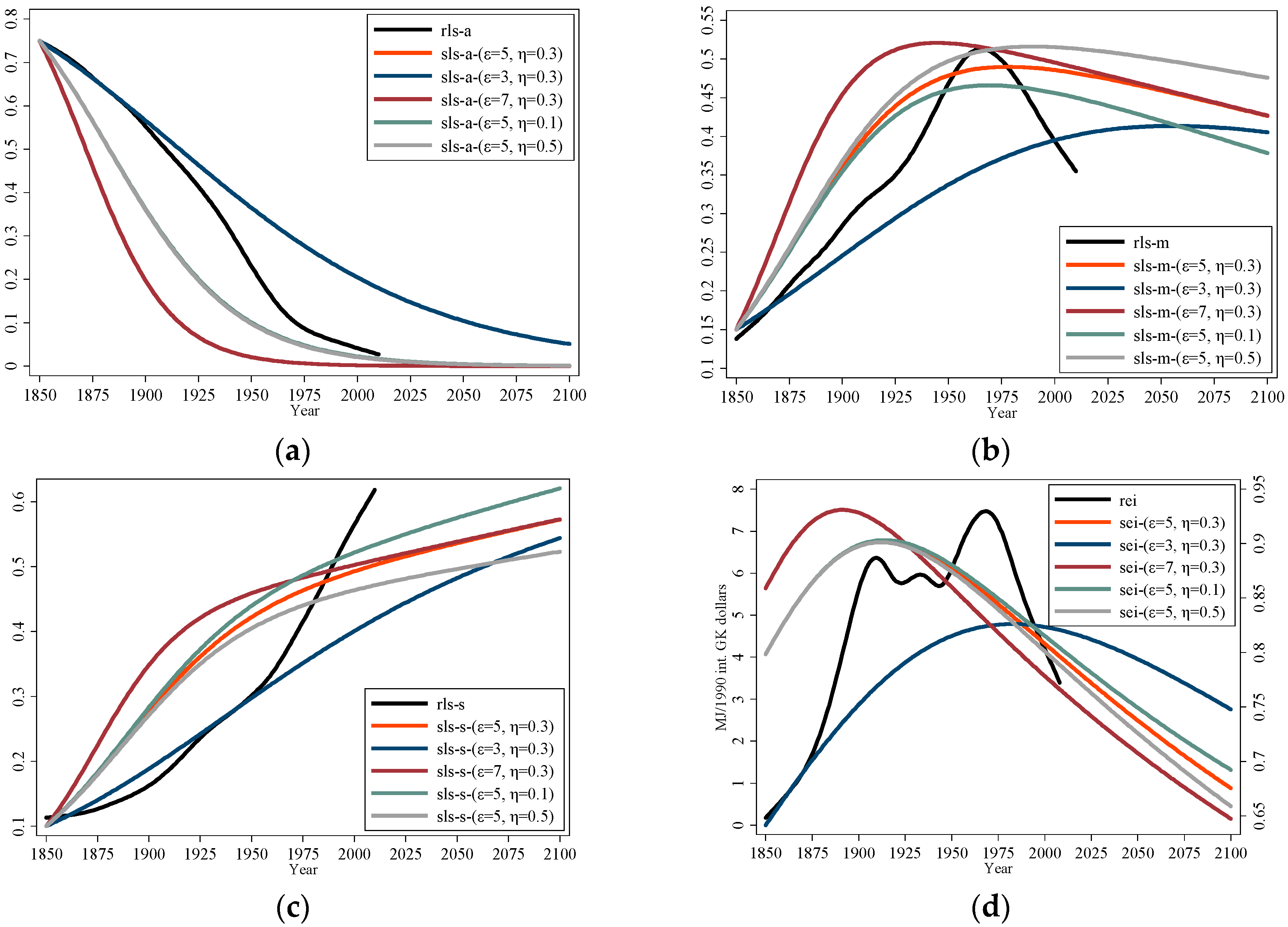
We first plot simulation results in Figure 2, where Figure 2a–c describes the long-run structural transformations of the three main industries according to Equations (17) and (21), and Figure 2d depicts the long-run change of economy-wide energy intensity with respect to the first expression in Equation (27). Further, there are five simulated scenarios concerning labor shares (i.e., simulated labor shares, sls) and energy intensity (i.e., simulated energy intensity, sei), according to different combinations. For the sake of comparison, we also plot in Figure 2 the real labor shares (rls) and real energy intensity (rei), which are calculated using Swedish historical data and smoothed by Hodrick–Prescott filter with a value of 1600.
For the baseline case ( and ), we can observe that the simulated changes of labor share in Figure 2a–c (agriculture, manufacturing and services, respectively) are in line with the predictions of Proposition 1 and also the Kuznets facts: the labor share of agriculture grows downward, the labor share of services grows upward, and the labor share of manufacturing grows upward first then downward. Still, we find that there are some differences between simulations and real facts as what Ngai and Pissarides [34] have shown in their Figure 5, implying that the mechanism of technological differences can explain structural change effectively but not completely since there also exist other competing mechanisms [53]. However, following this mechanism, the inverted-U development of overall energy intensity could be satisfactorily illustrated in Figure 2d. That is, the turning points of inverted-U appear in the reasonable range, and the real and simulated trends are generally matched.
Next, we investigate the impact of elasticity of substitution on structural and energy intensity changes. According to Equations (16) and (20) and Assumptions 1 and 2, we can conclude that the bigger
is, the faster labor share of agriculture (modern sector) declines (increases), and similarly, the smaller
is, the faster labor share of services (manufacturing) increases (declines) within modern sector. However, due to the nested CES function, the changes of labor share in manufacturing and services are determined by the relative power initiated by different elasticities of substitution. For example, in Figure 2a–c, compared to the baseline case ( and ), the curves of labor share become much steeper or smoother when becomes bigger () or smaller (), since just measures the substitution possibility between agriculture and modern goods. According to the variable technological growth rates in Equations (19) and (23), and the dynamics of modern and economy-wide energy intensity in Equations (26) and (27), the inverted-U curve of overall energy intensity in Figure 2d becomes steeper or smoother with an earlier or later peak if the substitution possibility between agriculture and modern sector becomes bigger () or smaller (). The underlying reason is that when becomes bigger, labor will flow faster out of agriculture to modern sector. Combined with Assumption 1, the final production growth rate in Equation (23) will become bigger, which results in a shorter time to peak the overall energy intensity in Equation (27).
On the other hand, when the substitution possibility between manufacturing and services grows bigger () or smaller (), the labor share curve of agriculture stays almost unchanged, while the labor share curves of manufacturing and services change significantly and oppositely (i.e., higher in manufacturing but lower in services compared with baseline case). That is, when grows bigger (), the flow of labor in modern sector (from manufacturing to services) will slow down, so that the labor share curve of services (manufacturing) becomes smoother (steeper) relative to the baseline case; on the contrary, when grows smaller (), the labor flow from manufacturing to services will speed up, which leads to a steeper (smoother) trend in the labor share of services (manufacturing). Accordingly, in Figure 2d, the inverted-U curve of economy-wide energy intensity becomes steeper (smoother) with an earlier (later) peak when becomes bigger (smaller).
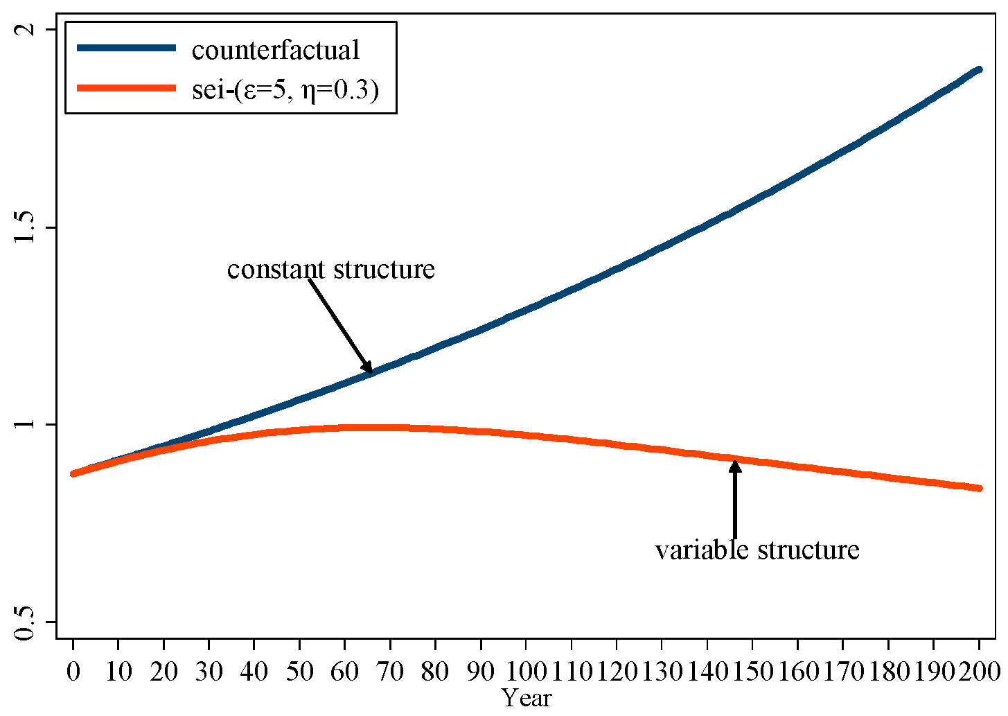
Second, we evaluate the relative effect of structural change on energy intensity change using the counterfactual analysis. According to the model economy, technological growth rates are exogenously given, so that the overall energy intensity will grow at a constant rate if the industrial structure keeps at the initial state. However, given technological differences among three main sectors as well as between main sectors and energy sector, structural change and sectoral energy intensity change will take place according to Proposition 1 and Equation (25), which might result in an inverted-U development of economy-wide energy intensity. Since sectoral energy intensity develops monotonically, it is structural change that may play the essential role in slowing down the increase of overall energy intensity and turning it downward.
Figure 3 provides a graphical illustration of this discussion, in which the inverted-U curve is intercepted from Figure 2d of the baseline case ( and ), and the line of “constant structure” is simulated through the counterfactual analysis without considering structural changes. In the case of “constant structure”, the economy-wide energy intensity is shaped only by Efficiency Effect, or the weighted sectoral energy intensities. Recalling that the initial labor shares in agriculture, manufacturing and services are 0.75, 0.15 and 0.1, respectively, and combing Assumption 3 of the specific changes of energy intensity in the three main industries, we can easily derive that energy intensity in agriculture dominates the development of economy-wide energy intensity and drives it upward over time. On the other hand, if structural changes are not restricted and distorted, that is, evolving following Proposition 1, we can instead observe an inverted-U curve of economy-wide energy intensity, which is determined by the mutual effect of sectoral energy intensity changes and structural changes. Furthermore, we find that structural changes in general represent the downward driving force on the development of economy-wide energy intensity, though it is not significant at the early period. In addition, relative effect of structural changes (downward force) to weighted sectoral energy intensities (upward force) is negative first and then becomes positive; accordingly, the economy-wide energy intensity increases until it peaks and then falls, like an inverted U. Overall, structural changes play a vital role in the slowdown of historical economy-wide energy intensity growth and also its downtrend.
5. Conclusions
This paper extends the models in Ngai and Pissarides [34] and Cao [33] through taking the heterogeneous elasticities of substitution into account. With a nested CES production function and some reasonable assumptions, we have deduced the typical path of structural transformation following Kuznets facts and provided an attempt to explain the inverted-U development of economy-wide energy intensity accompanied by structural transformation. Theoretical analysis indicates that: (1) if agricultural and modern goods are gross substitutes, manufacturing and services goods are gross complements, and the magnitudes of sectoral technological growth rates in manufacturing are the biggest, followed by services, and agriculture the smallest, the economy will experience typical structural transformation; (2) sectoral energy intensity change is determined by the difference of sectoral and energy threshold technological growth rates; and (3) if energy threshold technological growth rate is bigger than agricultural technological growth rate but not bigger than services technological growth rate, the economy-wide energy intensity will grow nonmonotonically like an inverted U.
We then apply Swedish historical data to calibrate parameters and simulate the typical structural transformation and the inverted-U change of overall energy intensity. The simulation exercises further show that: (i) elasticities of substitution may affect the shapes (steep or smooth) and peak periods (short or long) of the inverted-U curve, which can explain to a certain extent the heterogeneous transitions of economy-wide energy intensity developments in different economies; and (ii) if the industrial structure stays unchanged at the initial state due to some distorted policies, the economy-wide energy intensity may keep increasing even if there has sectoral and overall technological progress. However, if structural adjustments take place following the mechanism of technological differences, the trend of overall energy intensity may be reshaped from upward to downward.
Finally, future research could be made from the following aspects. On the one hand, even though our model has well explained the inverted-U change of economy-wide energy intensity, the predictions of sectoral energy intensity developments are somewhat less satisfactory. That might be because we do not take the nonmonotonic variations within sectors into account, or that we assume all the energy products to be homogeneous. For the latter case, due to the assumption of energy homogeneity, the energy technological growth rate stays unchanged over time, whereas in reality energy products are heterogeneous and have experienced a long-run transition. In view of this, a comprehensive model accommodating both structural change and energy transition could be explored in further study, through, e.g., incorporating energy transition models (e.g., [16,17,19,20,22]) into this present model. On the other hand, we only use Swedish historical data to test theoretical predictions, which might not be sufficient. If very long period data become available in other counties, the theoretical findings could be further examined in the future.
Supplementary Materials
The following are available online at www.mdpi.com/2071-1050/9/6/967/s1.
Acknowledgments
This paper is supported by the National Natural Science Foundation of China (Nos. 71273074 and 71673067).
Author Contributions
Lizhan Cao conceived and designed the research, and wrote this manuscript. Zhongying Qi participated in discussion and provided some important suggestions. All authors read and approved the final manuscript.
Conflicts of Interest
The authors declare no conflict of interest.
Appendix A
Proof of Proposition 1.
According to Equations (17) and (19), we provide the dynamics of the labor shares of manufacturing and services in the modern production:
Similarly, we give the dynamics of labor shares of agriculture and modern sectors:
Combining Equations (A1) and (A2), we obtain the dynamics of labor shares of manufacturing and services in the final production:
According to Assumptions 1 and 2, and , we derive:
Equation (A5) proves all the cases in Proposition 1 except the inverted-U change of labor share in manufacturing, which is provided as follows.
Rewrite the first expression in Equation (A1) into the following form:
Taking derivative with respect to on both sides of Equation (A6), we have:
Equation (A7) shows that the growth rate of the labor share of manufacturing is monotonically decreasing. Since the economic evolution is long enough, according to Equation (A5), we can reasonably derive that, when , then and hold. Accordingly, when , then and hold. Combined with Equation (A6), we get:
According to Equations (A7) and (A8), there exists only one , satisfying . As such, when , the labor share of manufacturing goes upward, while when , the labor share of manufacturing goes downward. Proposition 1 is proved. ☐
Proof of Proposition 2.
Referring to Equation (27), given
, the dynamics of overall energy intensity depends on the dynamics of final technological growth rate:
Taking the second derivative of with respect to , we get:
Recall Equations (A1) and (A2), we take derivatives with respect to and obtain:
Plugging Equation (A11) into Equation (A10), we derive , implying that is monotonically decreasing. We then reform Equations (A1) and (A2), and put them into Equation (A9). Considering the long enough evolutionary development, we get:
According to Equations (A10), (A12) and (A13), we can conclude that there exists only one , satisfying . That is, reaches its maximum at . Moreover, we can easily derive that, when then and when then . Referring to Assumption 3, we can deduce that there exists only one , satisfying . We then obtain for and for , indicating that the economy-wide energy intensity grows nonmonotonically like an inverted U. Proposition 2 is proved. ☐
References
- Reddy, A.K.N.; Goldemberg, J. Energy for the Developing World. Sci. Am. 1990, 3, 110–118. [Google Scholar] [CrossRef]
- Goldemberg, J. Leapfrog energy technologies. Energy Policy 1998, 10, 729–741. [Google Scholar]
- Henriques, S. Energy Transitions, Economic Growth and Structural Change: Portugal in a Long-Run Comparative Perspective; Lund University: Lund, Sweden, 2011; p. 113. [Google Scholar]
- McConnell, K.E. Income and the demand for environmental quality. Environ. Dev. Econ. 1997, 4, 383–399. [Google Scholar] [CrossRef]
- Jones, L.E.; Manuelli, R.E. Endogenous policy choice: The case of pollution and growth. Rev. Econ. Dyn. 2001, 2, 369–405. [Google Scholar] [CrossRef]
- Schumacher, I. The endogenous formation of an environmental culture. Eur. Econ. Rev. 2015, 76, 200–221. [Google Scholar] [CrossRef]
- Marsiglio, S.; Ansuategi, A.; Gallastegui, M.C. The environmental Kuznets curve and the structural change hypothesis. Environ. Resour. Econ. 2016, 2, 265–288. [Google Scholar] [CrossRef]
- Kander, A.; Malanima, P.; Warde, P. Power to the People: Energy in Europe over the Last Five Centuries; Princeton University Press: Princeton, NJ, USA, 2014; Available online: http://www.fas.harvard.edu/~histecon/energyhistory/energydata.html (accessed on 26 May 2017).
- Maddison, A. Statistics on World Population, GDP and Per Capita GDP, 1-2008 AD; University of Groningen: Groningen, The Netherlands, 2010; Available online: http://www.ggdc.net/maddison/oriindex.htm (accessed on 26 May 2017).
- Kijima, M.; Nishide, K.; Ohyama, A. Economic models for the environmental Kuznets curve: A survey. J. Econ. Dyn. Control 2010, 7, 1187–1201. [Google Scholar] [CrossRef]
- Dasgupta, P.; Heal, G. The optimal depletion of exhaustible resources. Rev. Econ. Stud. 1974, 41, 3–28. [Google Scholar] [CrossRef]
- Solow, R.M. Intergenerational equity and exhaustible resources. Rev. Econ. Stud. 1974, 41, 29–45. [Google Scholar] [CrossRef]
- Stiglitz, J. Growth with exhaustible natural resources: Efficient and optimal growth paths. Rev. Econ. Stud. 1974, 41, 123–137. [Google Scholar] [CrossRef]
- Stern, D.I.; Kander, A. The role of energy in the industrial revolution and modern economic growth. Energy J. 2012, 3, 125–153. [Google Scholar] [CrossRef]
- Solow, R.M. A contribution to the theory of economic growth. Q. J. Econ. 1956, 1, 65–94. [Google Scholar] [CrossRef]
- Kander, A.; Stern, D.I. Economic growth and the transition from traditional to modern energy in Sweden. Energy Econ. 2014, 46, 56–65. [Google Scholar] [CrossRef]
- Fröling, M. Energy use, population and growth, 1800–1970. J. Popul. Econ. 2011, 3, 1133–1163. [Google Scholar] [CrossRef]
- Galor, O.; Weil, D.N. Population, technology, and growth: From Malthusian stagnation to the demographic transition and beyond. Am. Econ. Rev. 2000, 4, 806–828. [Google Scholar] [CrossRef]
- Eren, E.; Garcia-Macia, D. From Wood to Coal May Well Be from Malthus to Solow. 2013. Available online: https://ssrn.com/abstract=2407255 (accessed on 26 May 2017).
- Pezzey, J.C.; Stern, D.I.; Lu, Y. From Wood to Coal: Directed Technical Change and the British Industrial Revolution. Available online: https://ssrn.com/abstract=2943773 (accessed on 26 May 2017).
- Acemoglu, D. Directed technical change. Rev. Econ. Stud. 2002, 4, 781–809. [Google Scholar] [CrossRef]
- Tahvonen, O.; Salo, S. Economic growth and transitions between renewable and nonrenewable energy resources. Eur. Econ. Rev. 2001, 8, 1379–1398. [Google Scholar] [CrossRef]
- Boyd, G.; McDonald, J.F.; Ross, M.; Hanson, D.A. Separating the changing composition of US manufacturing production from energy efficiency improvements: A Divisia index approach. Energy J. 1987, 2, 77–96. [Google Scholar]
- Ang, B.W. LMDI decomposition approach: A guide for implementation. Energy Policy 2015, 86, 233–238. [Google Scholar] [CrossRef]
- Gowdy, J.M.; Miller, J.L. Technological and Demand Change in Energy Use: An Input–Output Analysis. Environ. Plan. A 1987, 10, 1387–1398. [Google Scholar] [CrossRef]
- Su, B.; Ang, B.W. Multi-region comparisons of emission performance: The structural decomposition analysis approach. Ecol. Indic. 2016, 67, 78–87. [Google Scholar] [CrossRef]
- Wang, C. Decomposing energy productivity change: A distance function approach. Energy 2007, 8, 1326–1333. [Google Scholar] [CrossRef]
- Wang, C. Changing energy intensity of economies in the world and its decomposition. Energy Econ. 2013, 40, 637–644. [Google Scholar] [CrossRef]
- Kim, K.; Kim, Y. International comparison of industrial CO2 emission trends and the energy efficiency paradox utilizing production-based decomposition. Energy Econ. 2012, 5, 1724–1741. [Google Scholar] [CrossRef]
- Lin, B.; Du, K. Decomposing energy intensity change: A combination of index decomposition analysis and production-theoretical decomposition analysis. Appl. Energy 2014, 129, 158–165. [Google Scholar]
- Haas, C.; Kempa, K. Directed Technical Change and Energy Intensity Dynamics: Structural Change vs. Energy Efficiency. Available online: https://ssrn.com/abstract=2788055 (accessed on 26 May 2017).
- Acemoglu, D.; Aghion, P.; Bursztyn, L.; Hemous, D. The environment and directed technical change. Am. Econ. Rev. 2012, 1, 131–166. [Google Scholar] [CrossRef] [PubMed]
- Cao, L. The Dynamics of Structural and Energy Intensity Change. Discret. Dyn. Nat. Soc. 2017, 2017, 6308073. [Google Scholar] [CrossRef]
- Ngai, L.R.; Pissarides, C.A. Structural change in a multisector model of growth. Am. Econ. Rev. 2007, 1, 429–443. [Google Scholar] [CrossRef]
- Kuznets, S. Modern economic growth: Findings and reflections. Am. Econ. Rev. 1973, 3, 247–258. [Google Scholar]
- Kongsamut, P.; Rebelo, S.; Xie, D. Beyond balanced growth. Rev. Econ. Stud. 2001, 4, 869–882. [Google Scholar] [CrossRef]
- Percebois, J. Economie de l´énergie; Economica: Paris, France, 1989. [Google Scholar]
- Panayotou, T. Empirical Tests and Policy Analysis of Environmental Degradation at Different Stages of Economic Development. Available online: http://www.ilo.org/public/libdoc/ilo/1993/93B09_31_engl.pdf (accessed on 26 May 2017).
- Pasche, M. Technical progress, structural change, and the environmental Kuznets curve. Ecol. Econ. 2002, 3, 381–389. [Google Scholar] [CrossRef]
- De Groot, H. Structural Change, Economic Growth and the Environmental Kuznets Curve: A Theoretical Perspective. 2003. Available online: https://repub.eur.nl/pub/837/ (accessed on 26 May 2017).
- Cherniwchan, J. Economic growth, industrialization, and the environment. Resour. Energy Econ. 2012, 4, 442–467. [Google Scholar] [CrossRef]
- Baumol, W.J. Macroeconomics of unbalanced growth: The anatomy of urban crisis. Am. Econ. Rev. 1967, 3, 415–426. [Google Scholar]
- Acemoglu, D.; Guerrieri, V. Capital deepening and nonbalanced economic growth. J. Political Econ. 2008, 3, 467–498. [Google Scholar] [CrossRef]
- Alvarez-Cuadrado, F.; Long, N.; Poschke, M. Capital-Labor Substitution, Structural Change and Growth. Available online: https://ssrn.com/abstract=2799602 (accessed on 26 May 2017).
- Stefanski, R. Structural transformation and the oil price. Rev. Econ. Dyn. 2014, 3, 484–504. [Google Scholar] [CrossRef]
- Engström, G. Structural and climatic change. Struct. Chang. Econ. Dyn. 2016, 37, 62–74. [Google Scholar] [CrossRef]
- Schön, L.; Krantz, O. New Swedish Historical National Accounts Since the 16th Century in Constant and Current Prices. General Issues; Lund Papers in Economic History; Lund, Sweden. 2015. Available online: https://www.ekh.lu.se/media/ekh/legs/forskning/database/shna1300-2010/publications_shna/lup140.pdf (accessed on 26 May 2017).
- Kurose, K. The Structure of the Models of Structural Change and Kaldor’s Facts: A Critical Survey. Available online: http://webpark1746.sakura.ne.jp/jafee2015/pdf/KuroseKazuhiro.pdf (accessed on 26 May 2017).
- Gernrnell, N.; Wardleym, P. Output, productivity and wages in the British coal industry before 1914: A model with evidence from the Durham region. Bull. Econ. Res. 1996, 3, 209–240. [Google Scholar] [CrossRef]
- Kander, A. Economic Growth, Energy Consumption and CO2 Emissions in Sweden 1800–2000. Available online: http://lup.lub.lu.se/search/ws/files/4913240/1789938.pdf (accessed on 26 May 2017).
- Schön, L. Electricity, technological change and productivity in Swedish industry, 1890–1990. Eur. Rev. Econ. Hist. 2000, 2, 175–194. [Google Scholar] [CrossRef]
- Henriques, S.T.; Kander, A. The modest environmental relief resulting from the transition to a service economy. Ecol. Econ. 2010, 2, 271–282. [Google Scholar] [CrossRef]
- Dennis, B.N.; İşcan, T.B. Engel versus Baumol: Accounting for structural change using two centuries of USA data. Explor. Econ. Hist. 2009, 2, 186–202. [Google Scholar] [CrossRef]
Figure 1.
Long-run energy intensity change in selected developed countries.

Figure 2.
Structural transformation and the inverted-U change of economy-wide energy intensity: (a) agriculture; (b) manufacturing; (c) services; and (d) economy-wide energy intensity change.
Figure 2.
Structural transformation and the inverted-U change of economy-wide energy intensity: (a) agriculture; (b) manufacturing; (c) services; and (d) economy-wide energy intensity change.

Figure 3.
Relative effect of structural change on the economy-wide energy intensity change.


Table 1.
Long-run sectoral energy intensity in Sweden (1910/12 price level).
| Energy Use (PJ) | Value Added (Billion SEK) | Energy Intensity (PJ/Million SEK) | ||||||||
|---|---|---|---|---|---|---|---|---|---|---|
| Agr. | Manu. | Serv. | Agr. | Manu. | Serv. | Agr. | Manu. | Serv. | S/M | |
| 1850 | 0.090 | 0.310 | 1.370 | 0.363 | 0.110 | 0.186 | 0.248 | 2.818 | 7.377 | 2.618 |
| 1870 | 1.000 | 2.000 | 7.920 | 0.547 | 0.199 | 0.303 | 1.828 | 10.034 | 26.102 | 2.601 |
| 1971 | 24.568 | 491.352 | 208.825 | 0.867 | 11.477 | 6.932 | 28.327 | 42.812 | 30.125 | 0.704 |
| 2005 | 23.811 | 428.597 | 297.637 | 0.679 | 23.299 | 16.178 | 35.050 | 18.396 | 18.397 | 1.000 |
Note: (1) “Agr.”, “Manu.”, and “Serv.” denote agriculture, manufacturing (industry and construction) and services (transportation and communication, and private services), respectively. (2) Energy use in 1850 and 1870 are collected from Kander [50] (p. 202) represented by coal since other modern energy forms are null at those periods. Specifically, in view of services, the values in transports and services are 0.72 PJ and 0.65 PJ respectively, the latter of which are estimated following Kander’s description. It is the same case for 1870 when the values in transports and services are 4.8 PJ and 3.12 PJ respectively. On the other hand, energy use in 1971 and 2005 are calculated with the data in Henriques and Kander [52] (p. 277) and Kander et al. [8]. (3) The data of Value added is collected from Schön and Krantz [47] at 1910/12 price level. (4) The column of “s/m” denotes energy intensity in services relative to that in manufacturing.
© 2017 by the authors. Licensee MDPI, Basel, Switzerland. This article is an open access article distributed under the terms and conditions of the Creative Commons Attribution (CC BY) license (http://creativecommons.org/licenses/by/4.0/).
Share and Cite
MDPI and ACS Style
Cao, L.; Qi, Z. Theoretical Explanations for the Inverted-U Change of Historical Energy Intensity. Sustainability 2017, 9, 967. https://doi.org/10.3390/su9060967
AMA Style
Cao L, Qi Z. Theoretical Explanations for the Inverted-U Change of Historical Energy Intensity. Sustainability. 2017; 9(6):967. https://doi.org/10.3390/su9060967
Chicago/Turabian StyleCao, Lizhan, and Zhongying Qi. 2017. "Theoretical Explanations for the Inverted-U Change of Historical Energy Intensity" Sustainability 9, no. 6: 967. https://doi.org/10.3390/su9060967
Note that from the first issue of 2016, this journal uses article numbers instead of page numbers. See further details here.